River Freshwater Contribution in Operational Ocean Models along the European Atlantic Façade: Impact of a New River Discharge Forcing Data on the CMEMS IBI Regional Model Solution

Abstract

River freshwater contribution in the European Atlantic margin and its influence on the sea salinity field are analyzed. The impacts of using a new river discharge database as part of the freshwater forcing in a regional ocean model are assessed. Ocean model scenarios, based on the CMEMS (Copernicus Marine Environment Monitoring Service) operational IBI-MFC (Iberia Biscay Ireland Monitoring Forecasting Centre) model set-up, are run to test different (observed, modeled and climatological) river and coastal freshwater forcing configurations throughout 2018. The modelled salinity fields are validated, using as a reference all known available in-situ observational data sources. The IBI model application is proven to adequately simulate the regional salinity, and the scenarios showcase the effects of varying imposed river outflows. Some model improvement is achieved using the new forcing (i.e., better capture of salinity variability and more realistic simulation of baroclinic frontal structures linked to coastal and river freshwater buoyancy plumes). Major impacts are identified in areas with bigger river discharges (i.e., the French shelf or the northwestern Iberian coast). Instead, the Portuguese shelf or the Gulf of Cadiz are less impacted by changes in the imposed river inflows, and other dynamical factors in these areas play a major role in the configuration of the regional salinity.

1. Introduction

In the global water cycle, ocean-atmosphere surface net freshwater fluxes are balanced by ocean transport and land discharges within the oceans. The return of terrestrial runoff into oceans is mostly concentrated at the mouths of the world’s major rivers, and it locally provides significant freshwater inflows, forcing changes in sea water densities. Consequently, realistic estimates of land freshwater discharges into oceans are needed to globally study water budgets [1]. At regional and local scales, and very specifically on coastal and shelf areas, the river runoff contribution is a major forcing of the ocean dynamics, having a strong influence on water stratification [2]. Besides, it also introduces significant fluctuations in local circulation patterns, generating important buoyant freshwater river plume-like flow structures [3]. Thus, noticeable on-shelf baroclinic frontal areas are caused and maintained in time by the freshwater contributions of one or various major rivers discharging in nearby coastal areas. These areas, generally located in coastal shelf seas or into estuaries where currents patterns are governed by density differences between salt sea water and fresh river water are known as Region of Fresh Water Influence (ROFI, [4]). The discharged freshwater volume, and its temporal variability, impact on the local circulation of such ROFI areas, by means of different interactions between the linked buoyancy plume structure and any existing regional ambient flow features (i.e., major current flowing along the slope, currents linked to open sea dynamics, barotropic tidal shelf currents, or ocean transports responding to prevailing wind regimes [5,6]). The coastal freshwater inputs even modulate typical coastal effects, such as upwelling events [7], having major impacts on the productivity and the whole ecological environment [8].

Due to this key role played at different scales on the ocean system, there is a growing interest in including realistic freshwater signals coming from land in operational ocean model systems.

In global ocean and basin models, which are extensively used in climate prediction and reanalysis production, this freshwater input is crucial to maintain water balances and to reproduce salinity fields with realistic latitudinal gradients that affect climate signals such as the Atlantic Meridional Overturning transports [9]. It is important to note that these global ocean model applications are not fit-for-purpose for performing on coastal areas as many processes of paramount importance to reproduce shelf dynamics are parameterized, filtered out, or simply not included. Furthermore, due to the typical global model coarse resolution, coastlines are not realistically represented. This limitation of global ocean models to deal with coastal areas has conditioned the way to force such models with punctual freshwater river discharges. Since most global models cannot accurately represent river mouths or estuaries, the freshwater river contribution has been traditionally included by means of some modification in surface ocean-atmosphere water fluxes along coastal areas (mostly modifying the evaporation-precipitation (E-P) ratio along coastal model grid points, as proposed by Bourdallé-Badie and Tréguier [10]).

The use of coastal and river freshwater forcing derived from climatological data has been a primary, and still a very commonly accepted, approach in global ocean modeling. However, available databases and services that progressively provide better estimates of coastal runoff and river discharges have started to improve ocean model freshwater coastal forcing input. Several research initiatives and established services are focused on generating at a global scale up-to-date runoff and freshwater river discharge historical datasets. Dai et al. [11] compiled for community use a global dataset with monthly streamflow at farthest downstream stations for the world’s 925 largest ocean-reaching rivers; likewise, the service currently provided by the Global Runoff Data Centre [12], under the auspices of the World Meteorological Organization (WMO), delivers quality controlled “historical” databases, comprising daily and monthly mean river discharges from more than 9900 in-situ stations from 159 countries. The GloFAS-ERA5 (Global Flood Awareness System) operational global river discharge reanalysis [13] produces, consistently with the ECMWF ERA5 (European Centre for Medium-Range Weather Forecasts global reanalysis, version 5th) atmospheric reanalysis and using a river network, a global gridded data product (with a horizontal resolution of 0.1 degree and at a daily time step) that covers from 1979 to near-real-time (within a delay of 7 days).

However, when we move into coastal ocean modeling, approaches and needs are slightly different: in their review of coastal modeling science foundation, Kourafalou et al. [14] pointed out the need of applying very high-resolution models at coastal scales, able to accurately capture coastal features, and forced with realistic punctual river inflows to adequately reproduce the related dynamics occurring in ROFI areas. This demand in terms of high-resolution models is crucial when forecasting estuarine circulation. Model applications focused on estuaries show horizontal resolutions that range from kilometric scales (at coastal boundaries) to meters (within the estuary zones). These extremely high coastal model resolutions should be accompanied by a combination of ad hoc riverine and atmospheric forcing with appropriate temporal variability (being needed daily, and even higher temporal frequency data). Therefore, neither river discharge monthly climatological products nor coarse resolution watershed model estimations are fully satisfactory when used to force operational ocean coastal models [15].

Lately, the utility of dynamical model downscaling from the deep ocean, across the continental shelf and into the coastal areas, has been extensively demonstrated [16,17,18]. In the framework of the Copernicus Marine Environment Monitoring Service (CMEMS), a global ocean model together with a wealth of regional ocean model systems, are operationally running to deliver short-term forecast and multi-year reanalysis information on the physical and biogeochemical ocean for the global ocean and the European regional seas (CMEMS, 2020 [19]). Specifically, along the European Atlantic façade, CMEMS provides a regional service (besides its global one) for the so-called IBI area (Iberia-Biscay-Ireland regional seas [20]). These CMEMS IBI regional products, down-scaled from the CMEMS global ones, are aimed to characterize upper-ocean dynamics at finer scales and to provide better boundary conditions for very-high-resolution coastal models, embedded into IBI solution, used by other non-CMEMS downstream services (as pointed out by Le Traon et al. [21], among others, one of the goals of the CMEMS mission).

The latest review of the current European capacity in terms of operational marine and coastal modeling systems [22] maps the organizations and the operational model systems at regional and coastal scales across Europe and points out the sustained availability of CMEMS global and regional scale core products as a positive driver to favor proliferation of “downstream” services devoted to coastal monitoring and forecasting. Likewise, this review highlights the availability of different operational ocean models, covering in some cases overlapped areas.

The availability of different operational regional and coastal model solutions in some IBI areas is seen as an opportunity for on-going initiatives, such as the MyCoast Project [23]. This EU Interreg Atlantic Program project is aimed at enhancing the regional cooperation, taking benefit of synergies among existing operational oceanographic tools and services to develop improved coastal risk services to support marine safety, fight against pollution, and generally, to increase preparedness to extreme met-ocean coastal events. MyCoast develops and upgrades different risk tools, making them suitable for using different operational model solutions as inputs. In parallel to this interoperability enhancement, a multi-model intercomparison exercise was conducted to deepen the knowledge on the different model products used as forcing by the MyCoast risk tools, identifying differences and analogies between 9 operational regional and coastal model solutions on overlapping areas. This multi-model comparison exercise, operationally updated since 2018, shows general consistency among the models, especially for sea surface temperature (SST). However, noticeable differences in sea surface salinity (SSS), mostly on shelf areas, are found (see Figure 1).

These modelled salinity differences are particularly evident in ROFI zones, such as the northwestern Iberian shelf and the French shelf in the Gulf of Biscay, and seem mostly related to the diverse treatment that each operational ocean model system gives to the coastal and river freshwater discharge forcing. Indeed, Matulka et al. [24] inform that the approaches followed to include freshwater inputs in each operational forecast system, shown in Figure 1, vary from one model set-up to another, using: (1) data derived from daily observations taken in river flow stations (i.e., the MeteoGalicia MTG-ROMS set-up and the CMEMS IBI one, but this one using observations only for some of the major rivers), (2) daily freshwater discharges at river mouths produced by hydrological models (this is the case for IBI, especially for its five-days-ahead forecast run), (3) data derived from river discharge monthly climatology (a very common approach, fully or partially used in IBI, IMI-ROMS and SHOM-HyCOM operational ocean model set-ups), and finally, (4) the no river forcing option (in this case, used only by the IST-MOHID operational version, available when the study was performed). Independently of the approach used to include this freshwater signal, what seems clear is that having a non-optimal representation of this coastal and river freshwater forcing in ocean model set-ups can lead to biased simulated ocean states, jeopardizing the reliability of ocean forecasts, and diminishing forecast skill on ROFI areas.

The MyCoast multi-model intercomparison exercise is further proof of the necessity to improve coastal freshwater signals in operational ocean models. This need, already identified within the operational oceanographic community [22], includes improved standardized freshwater river inputs (considering not only flow rates but also particulate and dissolved matter key for biogeochemical processes) and foresees, as a longer-term objective, to include connection and coupling with land hydrology models.

Likewise, the CMEMS Service, as part of its Evolution Strategy and scientific research priorities (CMEMS Scientific and Technical Advisory Committee, 2017 [25]), identified the enhancement of land forcing within their medium- and long-term objectives.

CMEMS has supported in the last years different research projects on cutting-edge science and technological developments, needed to ensure future state-of-the-art service evolutions. Within the last call for tenders (2018–2020), two CMEMS service evolution projects were dedicated to make the required research to improve the freshwater river discharge inputs for global and regional CMEMS models: the BRONCO (Benefits of dynamically modelled river discharge input for ocean an coupled atmosphere-land-ocena systems) Project [26] was aimed at generating a global river discharge reanalysis, using the GloFAS system driven by the ECMWF ERA5 atmospheric reanalysis. On the other hand, the LAMBDA (Land Marine Boundary Development and Analysis) Project [27], regionally focused on the European Atlantic Façade and the North Sea, had the objective of achieving better estimations, by means of high-resolution hydrological model simulations, for characterizing major, and also some minor, river contributions and their day-to-day variability (highly needed for operational ocean coastal models). The resulting new freshwater model estimates, more realistic and adjusted using observations along historical periods, reproduce not only more reliable long-term changes in continental freshwater discharges into the oceans, but also a more detailed spatial distribution. These model products and in-situ observational data are operationally updated, made available and downloadable into the LAMBDA product viewer web interface (http://www.cmems-lambda.eu/mapviewer/ (accessed on 8 April 2021)).

The present work aims to quantify the potential added value of using this new LAMBDA freshwater discharge product as part of the fresh water forcing of a regional ocean model simulation. To this aim, different model scenarios, based on the CMEMS IBI model configuration, have been designed and run. The modelled salinity fields, resulting from the different sensitivity IBI test runs, are validated by means of comparison with different in-situ observational data sources. Despite that test runs are performed over the whole IBI model domain, this study mostly focuses on ROFI areas of the Atlantic Iberia and on the French shelf in the Gulf of Biscay.

2. Materials and Methods

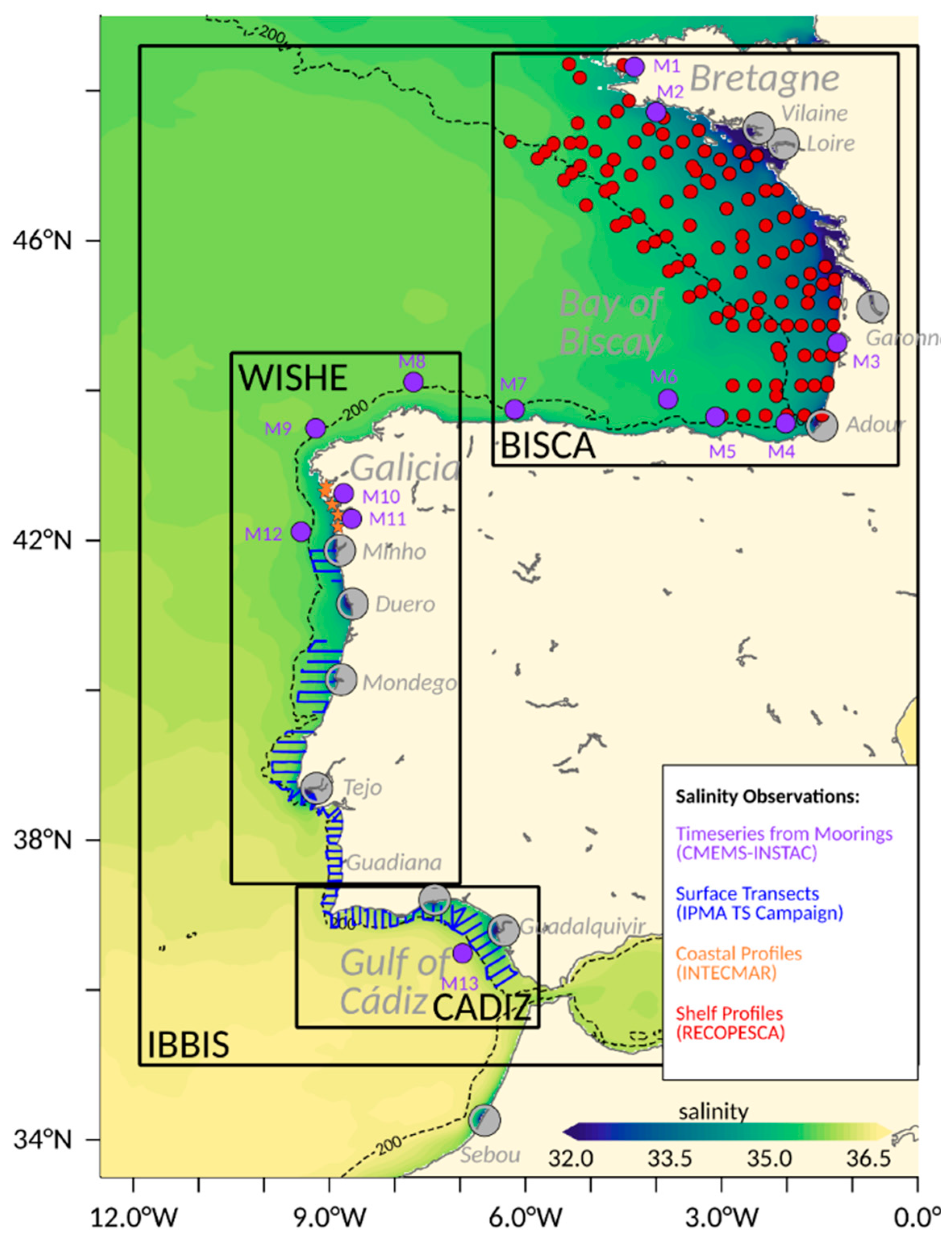
2.1. Description of Study Domain: In-Situ Observed Salinity Products

The region of study, hereafter referred as IBBIS, is a subset of the IBI operational configuration (Figure 2) and spans from the Strait of Gibraltar (35° N) to Bretagne (48.6° N). The warm and saline Iberian Poleward Current (IPC, [28]) flows along the steep slope of the narrow shelf of the Western Iberian Peninsula (50 km wide at its maximum, west of 8° W), then around the Galician shelf, and finally, enters the Bay of Biscay, separating the continental shelf waters from the open-ocean dynamics. This semi-enclosed Bay of Biscay features a narrow shelf on its southern part that widens towards the North (~150 km at 47° N), separated from a deep abyssal plain (more than 4000 m depth) by a steep and rugged slope, with many canyons. The main drivers on the shelf of this IBBIS domain are wind, tides and freshwater coastal runoff. The ocean dynamic varies locally, depending on the orientation of the coast, width of the shelf, freshwater discharge rates and other factors.

In this study, the IBBIS domain has been divided in three subregions, each one featuring its own characteristics: the CADIZ area, that is the Northern shelf of the Gulf of Cádiz, the Western Iberian Shelf (WISHE area), that includes the western shelf of the Iberian Peninsula, and the Gulf of Biscay (BISCA area).

The CADIZ area, at the southern tip of the Iberian Peninsula, is the place where the exchanges between the Atlantic and Mediterranean take place, across the Strait of Gibraltar. The saline MOW (Mediterranean Outflow Waters) come as a subsurface outflow from the Strait of Gibraltar, and cascade along the slope of the narrow shelf of the bay [29,30]. The circulation on the shelf is wind-driven, with a clear seasonal variability [31]: upwelling occurs in summer under the influence of northerlies, while downwelling takes place in winter under the influence of southerlies [32]. The variability on the shelf is explained by the front between the cold upwelled shelf-waters and the warmer southern waters (e.g., Reference [33]). Two main rivers, Guadalquivir and Guadiana, feed the shelf on its wider portion: in winter, the increased river runoff cools down the shelf waters [34] and contributes to the generation of a westward inshore flow [35], although this is not the main driver.

The WISHE area features a narrow shelf (30 to 90 km at its widest), and in comparison to the other proposed study subregions, this is the most sensitive to open-ocean general circulation patterns occurring in the North-eastern Atlantic. The geostrophic flow of the IPC intensifies in winter and isolates the narrow shelf’s waters from the open-ocean southward circulation. Along the Galician coast, the currents are mainly wind-driven [36]. The WISHE area marks the limit of the Eastern North Atlantic Upwelling region, with a frequent development of equatorward filaments at the coast in spring and autumn [37]. The interactions and front dynamics between the IPC and the shelf waters are complex [38]. The Western Iberian Buoyant Plume extends from the Mondego river northwards and is characterized by a salinity below 35.8. It is fed by the Mondego, Douro and Minho rivers and the numerous Rias of Galicia. Under non-upwelling conditions, the plume stays confined to the inner shelf and contributes to the stratification and cooling of the shelf waters. On the other hand, under upwelling conditions, the plume extends offshore, and masks the thermal signature of the IPC.

Finally, in the BISCA area, the IPC develops instabilities and eddies along its path which propagate offshore and take part of the general anticyclonic circulation of the open-ocean section [28,39]. On the French shelf, the main drivers are the coastal density-driven jets which interact with the tidal signal [40,41], and the surface wind-driven currents that advect shelf waters southward, e.g., Solabarrieta et al. [42]. In winter, the activity is weak over the shelf, but intense mesoscale activity takes place in the open ocean. The Southwestern winds induce northeastward drift over the shelf. From spring, the wind weakens and the dynamic activity on the shelf reaches the same levels of energy as offshore [43]. The major source of freshwater on the BISCA shelf is the river outflow, with a seasonal cycle featuring a maximum of discharge in winter and spring. The main rivers are the Loire and Vilaine system (47° N), the Garonne (45° N) and the Adour, in the South-West corner of the bay. Freshwater filaments extend from the coast and participate in the cross-shelf exchange [44]. Patches of low-salinity surface waters can be pushed by wind-induced coastal upwellings and reach the shelf-break [45]. Along the northern Iberian coast, the numerous rivers have a small averaged runoff, but can have peaks of torrential discharge, principally in spring and autumn. The accumulated outflow from these coastal rivers in winter and spring induces a low-salinity front on the narrow shelf [46], that can reach the shelf-break and extend down to 50 m depth [47].

All the in-situ salinity observations available for the year 2018 were gathered and explored to assess the capacity of the IBI model configurations to reproduce salinity fronts and river plume extension on the shelf, depending on each freshwater forcing.

Table 1. Overview of the in-situ observational salinity data sources in the study domain and subregions.

	Bay of Biscay (BISCA): 9.5 W–5.8 W/35.5 N–37.38 N	Western Iberian Shelf (WISHE): 10.5 W–7 W/37.4 N–44.5 N	Gulf of Cadiz (CADIZ): 10 W–6.5 W/43 N–48.5 N	Iberian-Biscay (IBBIS): 12 W–0 W/35 N–48.6 N
Hourly SSS Timeseries at Mooring Buoy	7 stations (M1 to M7, from N to S)	5 stations (M8 to M12, from N to S)	1 station (M13)	13 stations (M1 to M13, from N to S)
(Shelf) XBT salinity profiles	106 profiles	-	-	106 profiles
Weekly (Coastal) CTD salinity profiles	-	5 stations	-	5 stations
Surface (Shelf) salinityTransects	-	1 campaign (IPMA 28 April–20 May 2018)	1 campaign (IPMA 21 May–30 May 2018)	1 campaign (IPMA 28 April–30 May 2018)

shows an overview of the available observations used in each of the study areas.

Hourly timeseries of salinity from mooring stations for the year 2018 were obtained from the CMEMS in-situ observational product (Copernicus Marine In-Situ Tac Data Management Team (2019) [48]). The buoys are mostly moored on the shelf or at the shelf-break (see their locations, represented by purple dots, in Figure 2) and measurements are collected at surface and subsurface (mostly between 1 and 3 m deep). After processing, 13 stations are available at the whole study area: 7 in the BISCA zone (numbered M1 to M7, following the coast southwards from Bretagne to Galicia), 5 in the WISHE one (numbered M8 to M12, from North to South) and 1 in the CADIZ subregion (M13). Data from all of them have been used for the model validation, however some stations provide a limited exploitable input; in some cases, there is no more than a few months of data available (e.g., M4), whereas in other cases, the buoy is moored too close to the coast, not being fully useful for a meaningful validation of a regional model such as IBI (e.g., M3 or M10). However, as salinity observational data are sparse, it has been decided not to discard them, but use them with caution.

Weekly salinity profiles from 5 conductivity-temperature-depth (CTD) stations over the year 2018 located at Rias Baixas within the WISHE area were provided by the Instituto Tecnolóxico para o Control do medio Mariño de Galicia (INTECMAR). These CTD measures have been running since 1992 and the current INTECMAR oceanographic network is formed by 43 stations distributed along the Galician Coast [49]. These weekly campaigns are very coastal, with most of the stations in Rias and estuaries. The depth values are not uniform over the year, depending on the devices used to measure the data [50]. In this study, only samples from the 5 most offshore INTECMAR CTD stations (identified by orange stars in Figure 2) over the year 2018 are used, and these measurements are compared with daily modelled salinity profiles extracted, at the closet model grid point, from the different IBI model runs.

Surface Transects measured every 10 min with thermo-salinometers (TSG) installed on board of the research vessel Noruega were performed during the year 2018. Data from this specific campaign were provided by the Instituto Português do Mar e da Atmosfera (IPMA). Blue transects depicted in Figure 2 show the on-shelf measurements taken from 42° N southwards. This IPMA campaign covers part of the WISHE and CADIZ zones for a short time (from 28 April until 30 May 2018). The salinity is calculated as the salinity of the water inside the TSG and it represents salinity of the oceanic surface layer. Therefore, these measurements are used to validate the surface salinity extracted from the different IBI model simulations performed.

Daily salinity expendable bathythermograph (XBT) profiles are obtained from the Coriolis Ocean Dataset for Reanalysis for the Ireland-Biscay-Iberia region [51] real-time website (www.coriolis.eu.org (accessed on 8 April 2021)). These data are located on the shelf (red dots in Figure 2) in the BISCA area and are a part of the RECOPESCA (Réseau de mesure de l’activité de pêche spatialisé et de données environnementales à usage scientifique) Project campaigns (IFREMER; L’Institut Français de Recherche pour l’Exploitation de la Mer), which collect in-situ data in the Bay of Biscay onboard fishing vessels [52]. The salinity XBT profiles are compared to the daily modelled salinity profiles extracted from IBI simulations at the closest grid point.

2.2. Description of the New River Freshwater LAMBDA Database

The CMEMS Service Evolution LAMBDA project [27] aimed to improve land boundary conditions by coupling watershed models to ocean regional models. The project study area simulated the territories draining to the European Atlantic front and the North Sea, to provide boundary conditions to the CMEMS IBI and NWS (North West Shelves) Monitoring and Forecasting Centers, using the MOHID (Water Modelling System) Land model [53] with regular grids with a 0.05° horizontal resolution. The MOHID Land model, part of the MOHID Modeling System (http://www.mohid.com (accessed on 8 April 2021); [54]), is a physically based, spatially distributed, continuous, variable time step model for the water and property cycles in inland waters that allows simulation of single and multi-catchment simulations.

Each drainage basin domain was simulated for a 11-year period (1 January 2008–1 January 2019) using ERA5 reanalysis meteorology from the Copernicus Climate Change Service (https://climate.copernicus.eu/ (accessed on 8 April 2021)). These simulations resulted in the first LAMBDA data product, used in this study, consisting of daily flow and temperature values near the river mouth for a total of 54 main European rivers. In a second phase, 70 extra discharges for minor rivers in Western Iberia and 364 extra discharges for Ireland and UK domain were extracted to obtain a more comprehensive freshwater budget in these areas. However, these extra rivers included in a second release of the LAMBDA database are not fully validated yet and the model resolution (too coarse) used may be a limitation to accurately represent flows from such minor rivers. Therefore, in this work, only used freshwater data for rivers (the ones used currently as forcing of the IBI model application) included in the first release of the LAMBDA database was used. More information about the LAMBDA project products and results can be seen in Campuzano et al. [55].

2.3. The CMEMS IBI Salinity Model Product

The CMEMS-IBI Near-Real-Time forecast and analysis operational product [56] is generated daily by means of a NEMO model application [57], run over a regional grid (see geographical coverage in Figure 1) with a horizontal resolution of 1/36° (around 3 km) and 50 unevenly distributed z vertical levels. A best estimate of the ocean state (IBI analysis generated through a model run with data assimilation on a weekly basis) and a five-day-ahead forecast (daily updated free model run) are routinely produced for a number of hydrodynamic variables, among others: temperature, salinity, mixed layer depth, zonal and meridional velocity currents and sea surface height. While hourly-averaged estimations are provided for the sea surface, daily-averaged values are computed for the rest of the three-dimensional water column in the entire IBI regional domain. Hourly 3D physical forecast data, covering exclusively the continental shelf and coastal areas, are additionally delivered to foster the dynamical downscaling and subsequent implementation of coastal downstream services.

The CMEMS IBI system uses a SAM2-based (second generation of Mercator Assimilation System) data assimilation scheme [58] to enhance its predictive skills by constraining the model in a multivariate way with a wealth of observations: Altimeter data (i.e., along-track sea-level anomalies), in-situ temperature and salinity vertical profiles (from the CMEMS CORA—Coriolis Ocean Dataset for Reanalysis- 4.1 database) and satellite-derived sea surface temperature (OSTIA—Operational Sea Surface Temperature and Sea Ice Analysis- product) are regularly assimilated to estimate periodically initial conditions for numerical forecast simulation. The resulting product from this latest IBI analysis run is what is delivered as historical best estimates.

At the time of the experiment, the IBI ocean model operational simulation is forced by 3-h daily updated high-resolution (1/8°) meteorological conditions provided by the European Center for Medium-Range Weather Forecast (ECMWF). Lateral open boundary conditions for temperature, salinity and currents, imposed from daily outputs from the parent system (the CMEMS GLOBAL ocean forecast [59]), are complemented with 11 tidal harmonics built from the FES2014 [60] tidal model solution. Land freshwater forcing is included in the IBI operational model set-up. Discharged flows for 33 of the main rivers presented in the IBI area are considered. In-depth insights into this IBI coastal and riverine freshwater forcing are provided in the next section devoted to describing the IBI model sensitivity tests performed in this study. For further technical specifications of the CMEMS-IBI model solution, the reader is referred to Sotillo et al. [20] and Aznar et al. [61].

The multi-parameter skill assessment of this CMEMS IBI ocean forecast system is operationally conducted through the NARVAL (North Atlantic Regional VALidation) toolbox, which routinely monitors its performance and prognostic capabilities by computing a variety of quality indicators [62]. Both real-time (‘online mode’) and regular-scheduled (‘delayed-mode’) comparisons are performed using a wealth of independent observational sources as a benchmark, encompassing in-situ observations (collected by moorings, tide-gauges, drifters, gliders and Argo floats networks) and remote-sensed estimations (from satellites and high-frequency radars). For salinity field, the CMEMS-IBI model performance is evaluated using a multiple spatio-temporal scale adopting a multi-platform approach (see list of observational data sources used in the IBI validation in

Table 2. Summary of observational (Obs) platforms used in NARVAL (North Atlantic Regional VALidation) toolbox to validate IBI model salinity (* the climatology used is the World Ocean Atlas (WOA) 2013).

Obs Source	Obs Type	Vertical Coverage	Geographical Coverage	Temporal Frequency	Purpose
Mooring Buoys	In-situ	Surface	Mostly on shelf	Hourly	Validation
SMOS	Remote sensed	Surface	IBI domain	Daily	Validation
Argo profilers	In-situ	3-Dimensional	Open waters	Daily	Validation
Gliders	In-situ	3-Dimensional	Ibiza Channel	Daily	Validation
Climatology *	Gridded product	3-Dimensional	IBI domain	Monthly	Consistency

).

With respect to in-situ observations, the NARVAL software tool makes routine comparisons of CMEMS IBI salinity model products, extracting sea surface salinity timeseries on the grid points closest to the mooring buoy locations, and salinity profiles where Argo or glider observations are available.

Additionally, the IBI SSS field is validated using daily remotely sensed satellite estimations derived from the European Space Agency’s Soil Moisture and Ocean Salinity (SMOS) mission. In recent years, the SMOS products have steadily evolved to mitigate systematic biases detected in coastal areas [63], and today, they better portray plume patterns in major river basins [64,65]. However, in the IBI area, there is still room for improvement in these SMOS-derived products, especially in the operational ones and at very coastal areas where systematic biases are identified. The operational SMOS products’ limitations (not able to fully capture variability associated to minor coastal freshwater contributions) have conditioned their use in NARVAL to operationally assess IBI salinity product quality, focusing the validation only on deep open waters.

It is pointed out that recent updates of SMOS products, taking benefit of new LAMBDA Project developments, has resulted in a new 9-year (2011–2019) reprocessing of global SMOS SSS daily maps. This new dataset introduces significant improvements with respect to the operational and previous SMOS versions, tending to improve salinity gradients, preserving the small-scale ones close to the coast [66], and minimizing latitudinal and seasonal biases [67]. These improvements support the possibility of using this new SMOS satellite data as a salinity reference in model assessments, and the IBI-MFC has introduced it in NARVAL as an extra salinity data source for IBI delayed mode validations.

Highlights from the operational validation of IBI salinity products with in-situ observations and comparisons with the new SMOS satellite product are shown in Section 3.1.

2.4. Description of the IBI Model Sensitivity Tests Performed Using LAMBDA Product as Forcing

In the CMEMS IBI operational NEMO model set-up, inputs from 33 rivers are prescribed as a daily flux of freshwater (0.1 psu. The main rivers of the European Atlantic Shelf are considered (e.g., Garonne or Rhine, which have mean outflows larger than 1000 m³s⁻¹), but also smaller rivers which can present a strong temporal variability (e.g., Guadalquivir, whose flow is usually below 200 m³s⁻¹, but has peaks up to 6000 m³s⁻¹). To compensate the input from missing rivers, whose individual debits can be negligible but in total have a significant impact on the coastal salinity, a monthly climatological runoff (hereafter FWF_CRF) is applied all along the coast. It is derived from the same climatology used in the CMEMS GLOBAL configuration. The overall freshwater input, surface runoff and rivers, in the operational CMEMS IBI configuration during 2018, had a daily mean flow of 16 × 10³ m³s⁻¹, where river discharge accounted for 67%. The river discharge flows used in the reference CMEMS IBI configuration consist of a composite of observations and climatology (hereafter referred to as FWF_REF) provided by the GRDC (Global Runoff Data Centre; http://www.bafg.de/GRDC (accessed on 8 April 2021)), the French “Banque Hydro” dataset (http://www.hydro.eaufrance.fr/ (accessed on 8 April 2021)), simulations from the Swedish Meteorological Service (SMHI) E-HYPE ((HYdrological Predictions for the Environment)) hydrological model (http://e-hypeweb.smhi.se (accessed on 8 April 2021)) and observations gathered by the Previmer project. For further technical details on how freshwater forcing is included in the IBI operational forecast service, the reader is referred to Amo et al. [56].

Ten rivers discharge in the IBBIS area (Figure 1). Four of them are along the French coast (BISCA area), four in the Western Iberian shelf (WISHE area) and two in the Gulf of Cádiz (CADIZ area). Since April 2018, most of the river discharges were forced by a monthly climatology (FWF_CLM) or by an annual mean flow (in the IBBIS region, only the Mondego river), calculated from the reference forcing. The new forcing set that will be assessed in this study comes from the LAMBDA project watershed product (FWF_LAM), described above.

Table 3. Mean daily river discharge (m³s⁻¹) and cumulated discharge (10³ m³s⁻¹) over 2018 for each forcing set, in the full study domain (IBBIS) and the three subregions (BISCA, WISHE, CADIZ).

IBI Freshwater Discharge Forcing Data	Mean Daily (Cumulated) Freshwater Discharge in m3s−1 (in 103 m3s−1)
	BISCA 1	WISHE 2	CADIZ 3	IBBIS 1,2,3
FWF_REF (IBI_OP Reference Forcing)	1031 (2826)	624 (1709)	251 (687)	1906 (5223)
FWF_LAM (LAMBDA Forcing)	1876 (5141)	1017 (2787)	358 (982)	3252 (8910)
FWF_CLM (Climatology)	806 (2207)	486 (1330)	130 (355)	1421 (3893)
FWF_CRF (Coastal runoff climatology)	6 (463)	3 (261)	1 (57)	10 (843)

The rivers prescribed as forcing in the subregions are: ¹ Vilaine, Loire, Garonne, Adour. ² Minho, Douro, Mondego, Tagus. ³ Guadiana, Guadalquivir.

shows the mean daily and cumulated annual flow for each of the forcing datasets in the four areas. Mean daily flow of the LAMBDA forcing for year 2018 in the IBBIS area reaches 8910 m³s⁻¹, that is 70% more than the river input used for the IBI reference run (5223 m³s⁻¹) and 128% more than the climatological forcing (3893 m³s⁻¹).

Figure 3 shows the daily river discharge of the reference forcing (FWF_REF, blue line), LAMBDA river database (FWF_LAM, red line), climatology (FWF_CLM, cyan dashed line) and the extra coastal runoff (FWF_CRF, grey line), in the IBBIS domain and the three subdomains (BISCA, WISHE, CADIZ). For the IBBIS region, in the first months of 2018, the variability and intensity are equivalent in both the reference and the new LAMBDA datasets, with peaks of freshwater in January and March, though peaks are not always simultaneous (Figure 3a). From April onwards, the FWF_REF is mainly based on the climatology and shows a smooth decrease in total river debit from Spring up to August, when it reaches a minimum average daily flow of ≈2000 m³s⁻¹. LAMBDA features a minimum in summer too, associated with a reduced variability, but shows two important peaks in June and November, that do not exist in the IBI reference forcing. The difference between the two datasets is particularly important in BISCA (Figure 3b), where the mean river discharge is 1.8 times more important in the new forcing (Table 3).

The impact of using new river discharge forcing in CMEMS-IBI, and more specifically on the simulated salinity fields and frontal features linked to river plumes, will be evaluated through specific IBI-like model scenarios. To assess the performance of the numerical model and identify the main sources of uncertainty linked to the river runoff forcing in the model simulations, four scenarios forced by the previously described freshwater discharge parametrization were performed over the year 2018.

Table 4. IBI model scenarios: Overview of model runs with each specific treatment of river and coastal freshwater inputs.

IBI Model Scenario	River Discharge Forcing	Use of Extra Coastal Runoff	IBI Model Run Type and Main Features
IBI_REF	FWF_REF	Yes	Free run (from 1 January 2018 to 31 December 2018). Control run.
IBI_LAM	FWF_LAM	Yes	Free run (from 1 January 2018 to 26 December 2018). LAMBDA river forcing scenario
IBI_NOR	FWF_LAM	No	Free run (from 1 January 2018 to 26 December 2018). LAMBDA river forcing, but no Coastal runoff
IBI_CLM	FWF_CLM	Yes	Free run (from 1 January 2018 to 19 June 2018). River climatological forcing scenario
IBI_OP	FWF_REF	Yes	CMEMS IBI Operational product (from 1 January 2018 to 31 December 2018) Data Assimilation scheme included (weekly update from IBI Analysis). Used as reference.

shows an overview of the four IBI model land boundary scenarios: IBI_REF is the reference simulation forced by the reference river discharge forcing, and its parameterization is identical to the one used in the operational IBI configuration, IBI_LAM differs from IBI_REF by using the LAMBDA river database forcing, IBI_NOR is like IBI_LAM, but without adding the extra coastal runoff (i.e., the river discharge forcing is the only input of freshwater), and finally, IBI_CLM is a run forced by climatology. The latter scenario was simulated only over the first 6 months of 2018, because the reference run from April is using as forcing the same climatology.

All the IBI scenarios were performed with the same model parametrization and forcing datasets, excluding the freshwater forcing, as the CMEMS-IBI operational configuration. A spin-up run of 110 days was performed to generate the same initial condition for all model scenarios. The model started from rest (the 6 September 2017) with initial three-dimensional temperature and salinity fields taken from the CMEMS-IBI operational outputs. After this spin-up period, the model solution was evaluated as stable, showing on the 1 January 2018 velocity fields similar in magnitude and pattern to the CMEMS-IBI operational solution.

All the outputs from these IBI model scenario runs are delivered at hourly frequency for the sea surface, and at a daily frequency for the rest of the water column. Thus, to validate model salinity outputs, surface hourly model data have been used for comparison with mooring observed timeseries to take advantage of the higher temporal frequency of these available in-situ salinity observations. On the other hand, to compare with other observational data sources, such as the ones based on CTD or XBT profiles, daily model salinity outputs at the closest grid point and depth are collocated.

3. Results

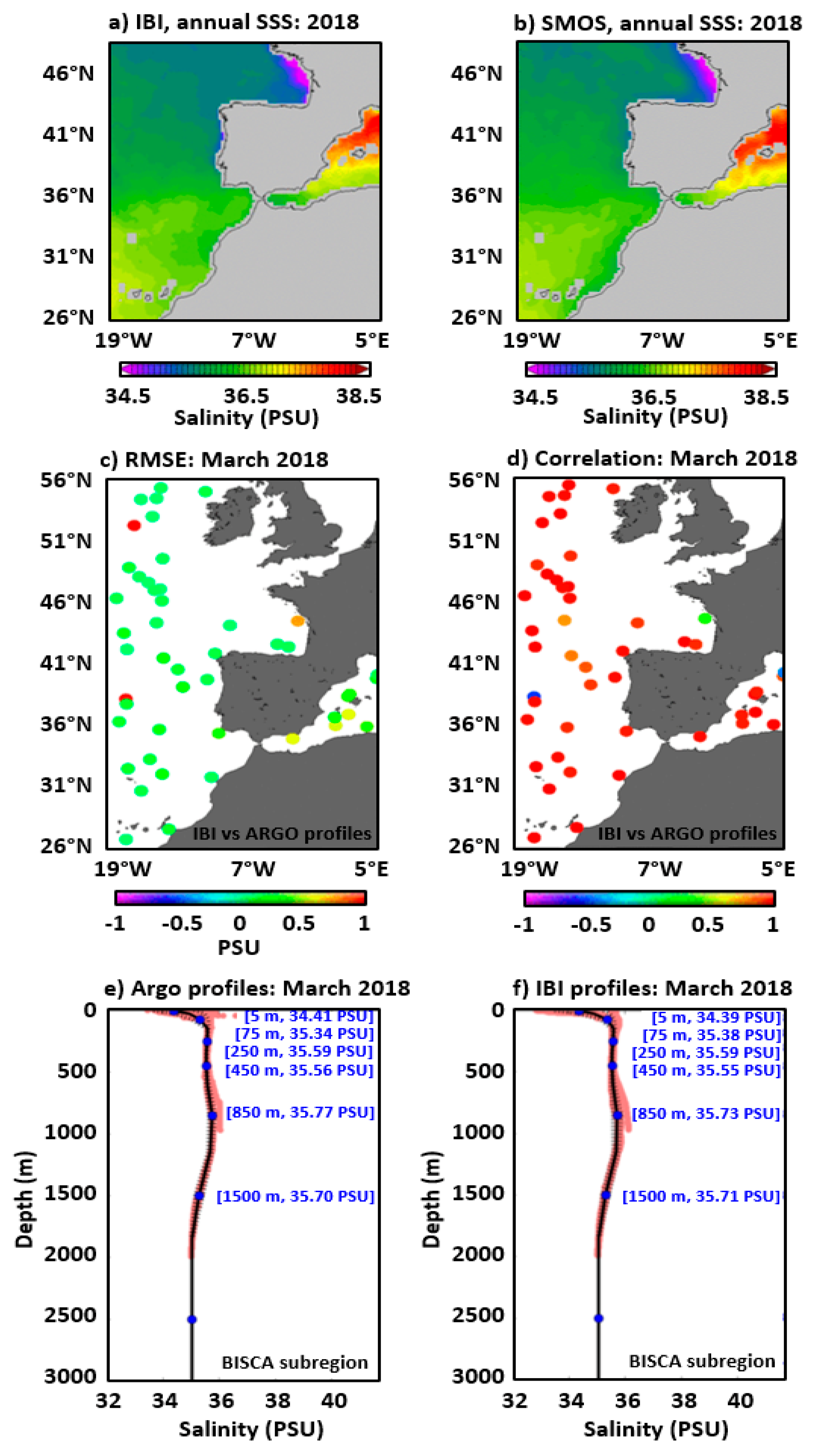
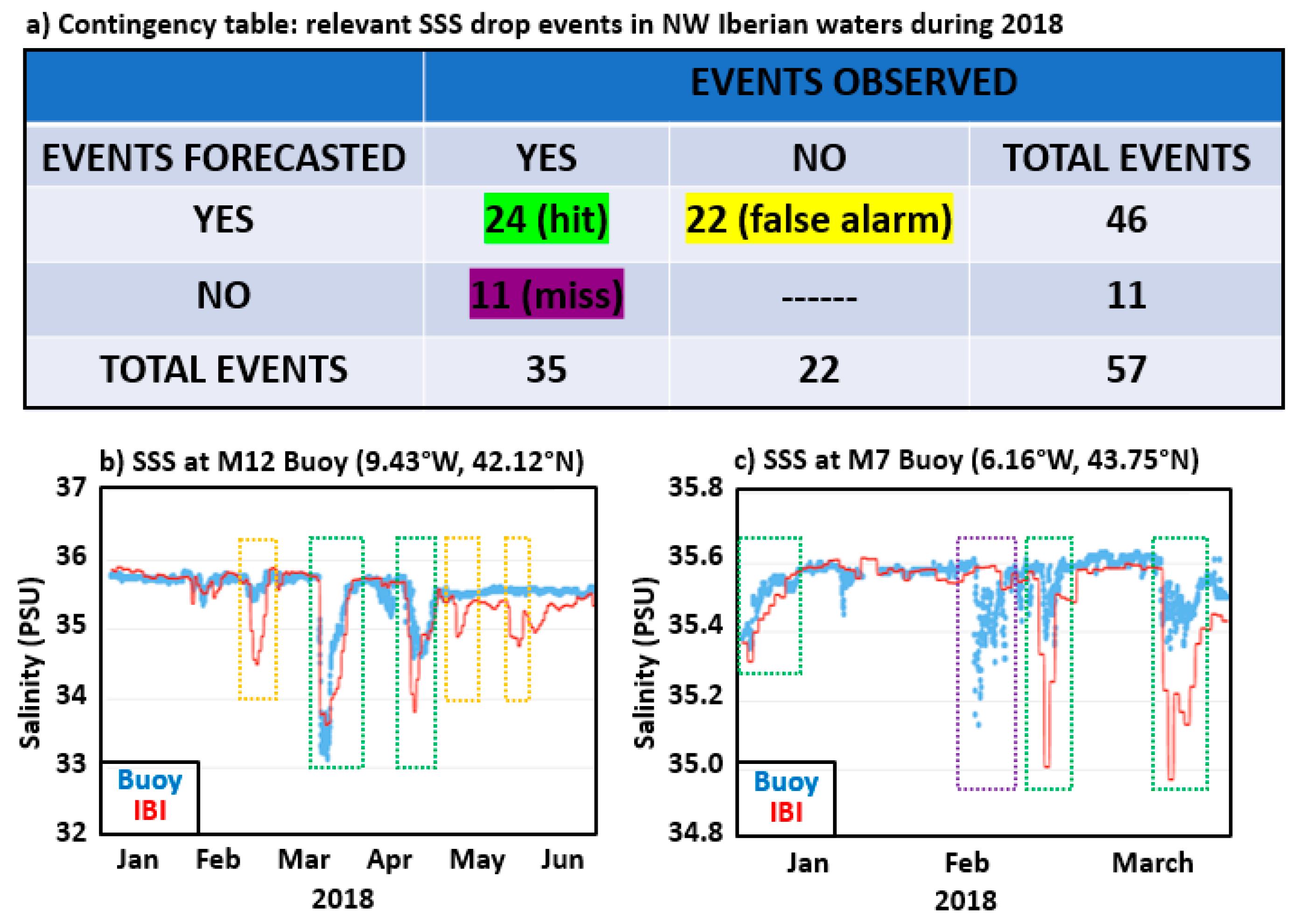
3.1. How Does the Operational CMEMS IBI Forecast Model Reproduce Salinity Fields?

In this section, and before analyzing specific results from the IBI model sensitivity tests performed, it is shown how the CMEMS IBI operational model system reproduced salinity fields for the study year (2018). NARVAL toolbox provided a wealth of outcomes and quality indicators on a monthly basis that allowed to quantify CMEMS-IBI prognostic capabilities to reproduce the salinity field during such year. Equally, “parent-son” model intercomparisons were regularly conducted with the purpose of checking the consistency of the CMEMS global solution and the regional downscaled IBI model solution, identifying any potential problem that might be inherited from the coarser global system. In this context, Lorente et al. [17] previously showcased the discrepancies in coastal areas during 2018 between the CMEMS IBI and its parent solution (CMEMS GLOBAL) due to the differences in both the horizontal resolution and the freshwater forcing implemented in their respective operational chains.

The CMEMS operational IBI performance appeared to be rather consistent, especially in open deep waters (Figure 4). The qualitative resemblance of yearly averaged maps of SSS for 2018 between the IBI model product and SMOS estimations was significantly high, with slight differences arising in nearshore shallower areas, especially in the African coastal upwelling region (Figure 4a,b).

With the aim of assessing IBI accuracy in the entire water column, quality-controlled salinity profiles collected by Argo floats were regularly used as a benchmark (Figure 4c–f). Monthly maps of skill metrics were computed by NARVAL toolbox for several depth layers and also for the entire full profiles, as exposed in Figure 4c,d. As it can be observed, moderate RMSE and high correlation values were obtained for March 2018, with most of the values emerging in the range [0–0.5] PSU and [0.71–0.93], respectively. Complementarily, monthly qualitative comparisons were conducted with a focus on specific subregions (Figure 4e,f). Here, the salinity profiles observed and modeled in the Gulf of Biscay are shown (the BISCA subregion displayed in Figure 2). Model outputs were vertically interpolated into the observation depth levels to facilitate the visual comparison. Likewise, averaged salinity profiles (solid black lines) were calculated to infer the main features of the water column in this area. According to the values for specific levels (in blue), the model-observations accordance was relevant for March 2018. Reduced differences were detected in the upper layer, where higher spatial-temporal variability of the salinity field is observed, lying between 33 and 36 PSU. Monthly statistical results for the rest of the year (not shown) illustrated that CMEMS IBI performance in off-shelf waters was consistent, operating within acceptable ranges all the year-long.

Since accuracy of SMOS remote-sensed estimations is higher in open offshore waters (these products showing a more limited precision in coastal areas mostly due to the lack of valid observations—this is so especially in the operational products and somehow minimized in the reprocessed ones) and Argo observations were constrained to offshore waters beyond the continental shelf, ancillary validation exercises with coastal buoys were required to objectively evaluate CMEMS IBI performance in the periphery of ROFI areas, where impulsive-type freshwater discharges might be noticeable. Using surface salinity observations from the coastal moorings available along the northwestern Iberian shelf (M5–M12 mooring buoys, depicted in Figure 2), a contingency table is served, not only as a summary of the most relevant SSS drop events occurred during 2018, but also as a qualitative overview of the CMEMS IBI model ability to adequately reproduce them (Figure 5a).

As it can be deduced from the contingency table, CMEMS IBI was able to represent 69% (24 of 35) of the episodes categorized here, with variable degreed of precision. By contrast, almost 50% (22 of 46) of the forecasted SSS drop events constituted false alarms, which were not confirmed by the in-situ observation. To better illustrate this validation approach, two examples at 2 buoys’ locations are provided (Figure 5b,c). In the first case, the 6-month SSS timeseries at Silleiro buoy (M12) location revealed a series of events, categorized as modelled hit and miss event (Figure 5b), chronologically described hereinafter:

• 22–28 February 2018: False alarm. IBI showed a SSS drop (more than 1 PSU), not so intense in the observed data.
• 20–30 March 2018: Hit. Both IBI and observed data exhibited a SSS drop (of more than 2 PSUs), with a very similar time evolution.
• 21 April–1 May 2018: Hit. Both IBI and Silleiro Buoy observation exhibited a SSS drop (about 2 PSUs), and the model overestimates the observed decrease.
• 10–14 May 2018: False alarm. IBI showed a non-observed SSS drop (around 1 PSU).
• 30 May–10 June 2018: False alarm. IBI showed a SSS drop around 1 PSU.

In the second case (Figure 5c), the 3-month comparison of SSS at Cabo de Peñas buoy (M7) location showed the following timeline features (hits and a miss event):

• 1–9 January 2019: Hit. Both IBI and observed data exhibited a moderate SSS drop of 0.5 PSU and a steady recovery during the following days.
• 13–17 February 2019: Miss. Observed drop of 0.5 PSU not reproduced by IBI.
• 25–28 February 2019: Hit. IBI clearly overestimated the observed SSS drop.
• 20–26 March 2019: Hit. IBI clearly overestimated the observed SSS drop.

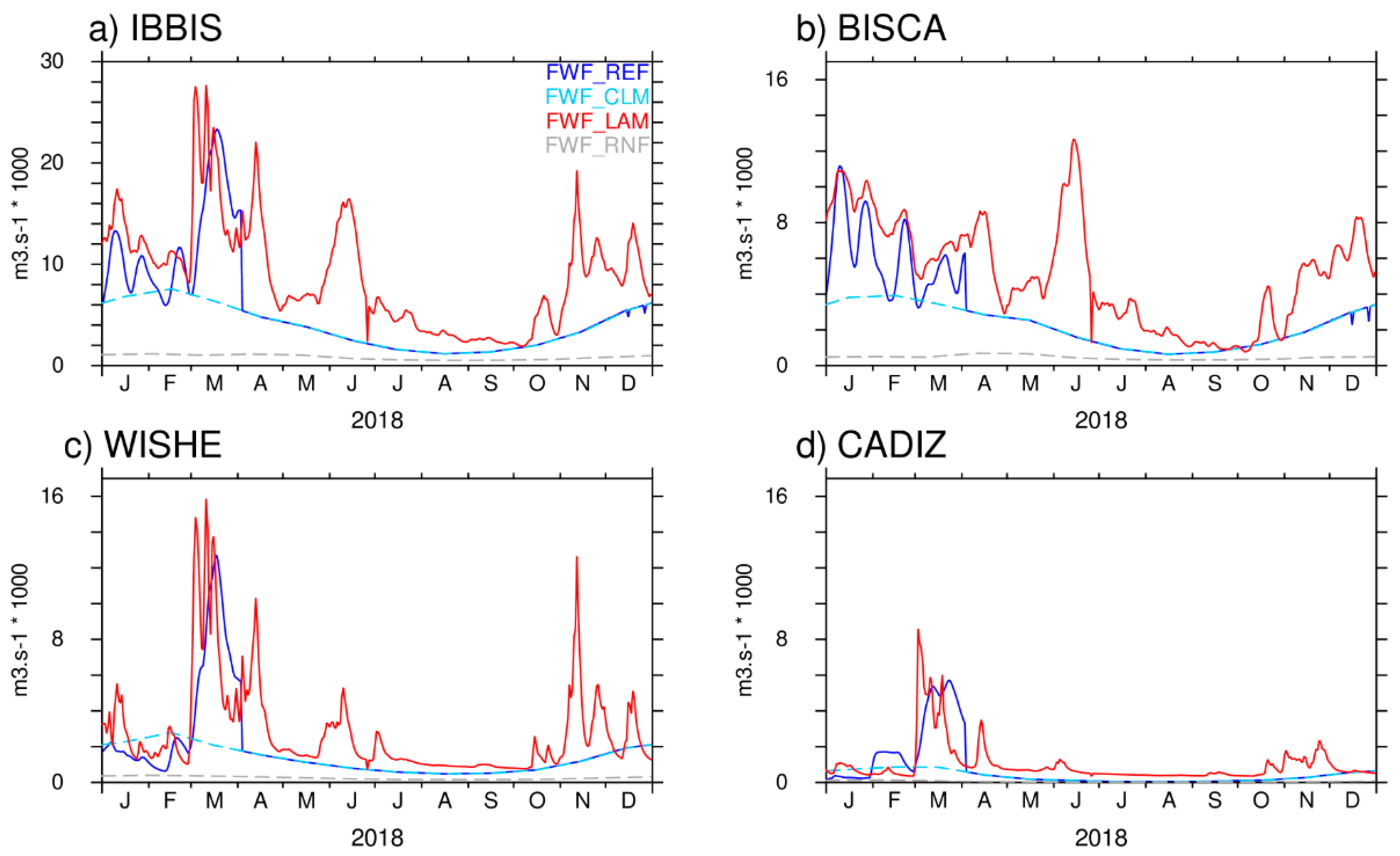
3.2. IBI Model Sensitivity to Changes in Freshwater Coastal and River Forcing

This section shows the main results of the IBI modeling scenarios performed to evaluate the regional impact on salinity after using different river/coastal freshwater forcing. In order to assess the four different IBI scenarios performed and to identify the main sources of uncertainty linked to the use of different river runoff forcing, the modelled outcomes have been validated with different in-situ salinity observations.

Figure 6 shows the seasonal SSS of IBI_REF, and the mean difference with the other simulations. In winter, that is the first 3 months after the start of the runs, the differences in the surface salinity field between the various simulations are limited to the shelf, and more specifically to the ROFI areas. Due to the higher river discharge of LAMBDA, IBI_LAM and IBI_NOR are fresher than IBI_REF. The same patterns are found in autumn. The small differences observed offshore at this time come from the expected propagation of the differences within the domain after 12 months of simulation but confirm that there is no noticeable bias appearing with any of the forcing sets. In spring and summer, the river discharge of LAMBDA is stronger than the other sources (as seen in Figure 3) and the fresher water masses of the two simulations forced by LAMBDA (IBI_LAM and IBI_NOR) extend to the open ocean, especially in the BISCA area. The Vilaine and Loire river system (at 47° N) impacts the surface and subsurface layers all year-long. The southernmost section of BISCA is the most sensible to the impact of the coastal runoff, as shown by the higher salinity of IBI_NOR in this area.

The simulation forced by a climatology (IBI_CLM) is saltier than the other simulations (+0.05 PSU over the IBBIS domain compared to IBI_REF) in winter. This emphasizes the fact that using a climatology vs. realistic daily river discharge significatively changes the salinity budget on the shelf.

These mean SSS seasonal snapshots from the test simulations show differences in the salinity patterns. Furthermore, it is needed to validate the simulated salinity fields against observations in order to assess the impact of these changes in the freshwater forcing.

The comparison with observed salinity timeseries from moorings shows that all the simulations globally manage to accurately reproduce the spatial-temporal variability of salinity at the coast and at the shelf-break, within the IBBIS domain (Figure 7). The correlations between mooring measurements and model scenarios outputs are most of the time above 0.6, and the standard deviation below 0.5 PSU. The capacity of the IBI model to reproduce the salinity is more explained by the geography and resolution of the local dynamics than by the parametrization of the river forcing: it can indeed be seen on the Taylor diagram (Figure 7a) that points are gathered by station, rather than being gathered by simulations. The simulation forced 6 months by the climatology differs most of the time from the others: it may be explained by the impact of a diurnal vs. climatological freshwater discharge forcing or by the shorter length of the simulation (6 months vs. 1 year).

As each subregion features its proper dynamics and local processes, the assessment of the salinity variability and fronts location, and the assessment of the impact of the river discharge forcing on the IBI configuration, have been conducted separately in BISCA, WISHE and CADIZ areas.

3.2.1. BISCA Region

The BISCA area is sensible to the open-ocean dynamics in its Southern part, where the shelf is narrower and the poleward slope-current is close to the coast. Where the shelf is wider, in the French shelf area, the tides and the freshwater runoff are the dominant factors. This local variability shows in the mooring’s measurements: in the northern part (M1 and M2, in Bretagne), the salinity is steady in summer and autumn, when stratification occurs. In the southern section (M5 to M7), the variability is, on the contrary, strong in spring/summer, when the mesoscale activity on the shelf is at its maximum (such as M6, Figure 7b). The simulations are all coherent with these local seasonal patterns. In the case of the station M6, IBI_CLM features an unrealistic variability in winter, that tends to support the hypothesis that a climatological river forcing degrades the solution in terms of variability, compared to a diurnal one.

The RECOPESCA campaign took place from 24 April to 30 May 2018. Even though its temporal coverage is limited to one month, it covers the whole French shelf and allows to estimate the extension of the ROFI (Figure 8). The low-salinity front does not reach the shelf break on the wider part of the shelf (north of 46° N). All the simulations overestimate the offshore extension of the ROFI, but the run forced by a climatology which, as seen from the in-situ timeseries, degrades the variability of salinity, features a smaller bias at the time of the campaign (1.55 PSU at the surface) than the other simulations. We can hypothesize that all the “realistic” river forcing data introduce too much discharged water on the shelf and/or do not manage to evacuate it. Nevertheless, validation of the salinity field is difficult because of the great variability of salinity on the shelf in the BISCA area due to large inputs of fresh water and strong variability.

The combined input from the extra coastal runoff and LAMBDA (IBI_LAM) creates a significant fresh pool of water on the shelf, particularly in the South, which degrades the solution at the time of the RECOPESCA campaign (Figure 8 and

Table 5. Mean difference (Bias) and Root Mean Squared Error (RMSE) between observed salinity (from mooring buoys and RECOPESCA XBT profiles) and simulated one (from the IBI_REF, IBI_LAM, IBI_CLM, IBI_NOR model scenarios), over the respective length of the simulations, in the BISCA area. The smallest model bias and RMSE for each dataset are in bold. The mooring data have hourly frequency and RECOPESCA data daily frequency. N is the number of measurements.

Salinity Observations in BISCA			RMSE				Bias (Model Observations)
			IBI_REF	IBI_LAM	IBI_CLM *	IBI_NOR	IBI_REF	IBI_LAM	IBI_CLM *	IBI_NOR
Mooring (2018)	Depth (m)	N
M1	5	8314	1.18	1.21	1.35	1.54	0.16	0.04	0.75	0.97
M2	1	3622	0.96	1.58	0.64	1.22	−0.72	−1.36	−0.52	−0.94
M3	1	6633	2.68	2.63	2.47	3.71	1.28	1.14	1.33	2.88
M4	10	2701	0.78	1.18	0.91	1.59	−0.65	−0.92	−0.69	−1.12
M5	3	6938	0.31	0.49	0.39	0.28	−0.11	−0.28	−0.13	0.00
M6	3	8160	0.24	0.38	0.15	0.19	−0.11	−0.24	−0.04	−0.03
M7	3	7022	0.32	0.30	0.48	0.38	0.18	0.11	0.22	0.29
RECOPESCA (May 2018)	Depth (m)	N
	0	106	1.69	2.14	1.55	1.79	−0.76	−1.24	−0.52	−0.79
	5	106	0.99	1.39	0.74	1.14	−0.67	−1.03	−0.39	−0.71
	10	106	0.47	0.61	0.46	0.56	−0.21	−0.32	−0.03	−0.21
	20	106	0.38	0.43	0.28	0.39	−0.20	−0.25	−0.10	−0.19
	50	106	0.11	0.09	0.09	0.09	−0.06	−0.06	−0.05	−0.04

* IBI_CLM timeseries are shorter than the others.

). However, by removing the extra coastal runoff (IBI_NOR), the solution is improved. The same observation can be made from the moorings’ timeseries: the simulation run with LAMBDA but without extra coastal runoff locally improves the solution, meaning that the salinity bias does not come from the LAMBDA forcing itself. In fact, the extra coastal runoff is not needed anymore on the southern shelf of Biscay, as the freshwater discharge is more realistic, even though it is still needed in other areas, where rivers are not parametrized (such as Brittany in the northern BISCA). A full network of coastal salinity observations would be optimal to tune this extra monthly runoff.

3.2.2. WISHE Region

The salinity at the shelf-break of WISHE is validated by comparison against the mooring stations M8, M9 and M12, all situated in the Northern part of the area. Here, salinity is steadier than in the BISCA area and it is mainly controlled by the slope current. However, occasional episodes marked by the advection of lower salinity water masses coming from the shelf (and highly modified by river and coastal freshwater influence) are clearly identified in the mooring sites. As previously commented in the description of the CMEMS salinity product validation, the IBI operational system can capture to some extent such noticeable surface salinity drops occurred in the peripheries of ROFI areas (see the forecast contingency table shown in Figure 5 in Section 3.1). Likewise, the IBI model scenarios generally accurately reproduce these observed freshwater intrusions, with small variations in timing and/or intensity.

As an example, Figure 9 shows the salinity from March to May 2018 at the western shelf-break of Galicia (station M9). A first well-marked event occurred on 20 March 2018 and has been documented by Campuzano [68] and Lorente et al. [17], and a second one less clearly defined occurred around 22 April 2018. This event of low-salinity intrusion at the shelf-break took place all around the Galician shelf (indeed, the same salinity drop event was also observed at the M12 station for the same period, see Figure 5b). All the IBI model simulations capture the events, at both locations, but show different performance characteristics. Thus, IBI_LAM is clearly too fresh during the first SSS drop event, but it is the only model run to replicate the low-salinity minimum observed on 30 April 2018. On the other hand, IBI_REF seems to be the only simulation to accurately capture the salinity drop on 14 April 2018. Finally, IBI_CLM is systematically too salty and IBI_NOR features a false salinity drop on 22 April 2018 at M12, further south (figure not shown).

Snapshots of model salinity fields at the dates when salinity dropped are observed in-situ (figures not shown) and indicate that these recorded events of low salinity are caused by filaments of freshwater, extending from the shelf towards the open ocean. The model simulations, actually all of them, feature these freshwater filaments, but with small spatiotemporal variations (of the order of a day or a few kilometers), meaning that at a given location (such as the mooring station), missing an event can be a matter of a few model grid points. Essentially, the resolution of this dynamical scale is stochastic, and a systematic resolution cannot be expected from a regional configuration such as the IBI one. However, this assessment shows that the IBI model configuration can catch the level of dynamical activity, with all model scenarios reproducing main salinity drop events. Once again, we emphasize that the use of a climatology slightly degrades the variability (timing and intensity) of the salinity.

In order to complete the analysis in this area, the weekly salinity profiles obtained from the INTECMAR CTD station records are used, located at same latitude as moorings M10 and M11. These observations are very coastal and taken at the mouth of the Rias Baixas in Galicia. This area is affected by freshwater plumes originating from discharges of several rivers [49], which are not parameterized in the IBI model set-up as proper river sources, but somehow it should be taken into account by means of the extra coastal runoff climatological forcing.

For validating the IBI model scenarios, simulated salinity profiles at the closest model grid point are vertically interpolated into the depth levels of the observations. All the simulations accurately reproduce the variability of salinity with observed data: steady in summer, but with salinity drops in winter and spring, affecting the whole water column in March and April.

Table 6. Mean difference (Bias) and Root Mean Squared Error (RMSE) between observed salinity (from mooring buoys, an IPMA campaign with thermo-salinograph and INTECMAR CTD stations) and simulated one (from the IBI_REF, IBI_LAM, IBI_CLM, IBI_NOR model scenarios), over the respective length of the simulations, in the WISHE area. The smallest model bias and RMSE for each dataset are in bold. The mooring data have hourly frequency, the IPMA data was measured every 10 min and INTECMAR measurements at each CTD station have a weekly frequency. N is the number of measurements.

Salinity Observations in WISHE			RMSE				Bias (Model Observations)
			IBI_REF	IBI_LAM	IBI_CLM *	IBI_NOR	IBI_REF	IBI_LAM	IBI_CLM *	IBI_NOR
Moorings (2018)	Depth (m)	N
M8	3	8587	0.16	0.13	0.09	0.19	0.12	0.10	0.06	0.15
M9	3	8676	0.19	0.20	0.13	0.17	0.06	0.03	–0.01	0.08
M10	3	6981	13.1	13.0	17.7	13.48	9.2	8.9	14.0	9.62
M11	9	6835	1.43	1.99	1.64	1.19	−0.93	−1.35	−0.96	−0.24
M12	3	8701	0.28	0.34	0.91	0.38	−0.03	−0.10	−0.05	−0.01
IPMA	Depth (m)	N
	surface	1563	0.51	0.73	0.50	0.64	−0.14	−0.18	−0.06	0.01
INTECMAR		N
C1		41	0.35	0.45	0.47	0.32	0.15	0.25	0.20	0.02
C2		38	0.50	0.62	0.78	0.48	0.14	0.26	0.17	0.03
C3		48	0.36	0.51	0.55	0.43	−0.06	0.07	−0.14	−0.04
C4		45	0.39	0.53	0.45	0.38	0.05	0.14	0.07	−0.01
C5		45	0.48	0.66	0.59	0.51	0.10	0.21	0.09	0.04

* IBI_CLM timeseries are shorter than the others.

shows statistics for the model validation at the 5 CTD INTECMAR stations. Figure 10 shows temporal evolution of observed and modelled salinities at the INTECMAR station C3 (8.96° W/42.48° N), showing a negative bias for all simulations in winter and the beginning of spring (stronger in November and December for IBI_LAM simulation), and a positive bias in the month of April (stronger for IBI_CLM simulation). Statistically, the simulation without extra coastal runoff has a better variability than the other simulations, with a correlation most of the time better than the other test simulations at both the INTECMAR stations and at the mooring buoy station, and also a smaller bias. It seems that by removing this extra local freshwater input, the simulated variability of salinity is improved. This fact can suggest that the salinity budget in this coastal point is rather controlled by the extension and variability of the western Iberian Buoyant Plume (mainly supplied and controlled by discharges of the Minho, Duero and Mondego rivers) than by the local runoff from the nearby Rias.

There are no timeseries of observed salinity from mooring buoys on the southern part of the WISHE area. However, the IPMA campaign recorded surface salinity transects across the Portuguese shelf, going South from 42° N. These thermo-salinometer measurements (taken from 28 April to 20 May 2018) have been used to validate the different IBI model scenarios in the area. Figure 11 shows how all the simulations have a negative surface salinity bias from 42° N to 39.5° N and at the Tejo river mouth, but inversely are too salty on the southern part of the measured area. As all the model scenarios feature the same pattern of bias in the region, it seems that the river discharge forcing data source is not the main cause of salinity errors on the shelf freshwater budget, with there being other dynamical factors that may explain this model behavior.

3.2.3. CADIZ Region

At the northern shelf-break of the Bay of Cádiz, we know from the data at mooring M13 that the salinity is steady around 36.5 PSU, except in summer when some small freshwater intrusions occur (±0.2 PSU, Figure 12b). The simulations have a correct average salinity here (less than 0.2 PSU of bias,

Table 7. Mean difference (Bias) and Root Mean Squared Error (RMSE) between observed salinity (from the M13 mooring buoy and the IPMA campaign) and simulated one (from the IBI_REF, IBI_LAM, IBI_CLM, IBI_NOR model scenarios), over the respective length of the simulations, in the CADIZ area. The smallest model bias and RMSE for each dataset are in bold. The mooring data have hourly frequency and IPMA data was measured every 10 min. N is the number of measurements.

Salinity Observations in CADIZ			RMSE				Bias (Model Observations)
			IBI_REF	IBI_LAM	IBI_CLM *	IBI_NOR	IBI_REF	IBI_LAM	IBI_CLM *	IBI_NOR
Mooring (2018)	Depth (m)	N
M13	3	8587	0.45	0.37	0.21	0.41	−0.19	−0.20	−0.15	−0.17
IPMA (May 2018)	surface	1217	0.59	1.18	0.42	1.12	−0.50	−0.87	−0.28	−0.71

* IBI_CLM timeseries are shorter than the others.

), but they reproduce punctual spurious intrusions, associated with peaks of river discharge. For instance, the strong river discharge of the reference forcing in February (Figure 3) has induced an extension of the ROFI up to the station, which is not realistic and only reproduced by IBI_REF. The same kind of behavior is observed in IBI_LAM in November.

While the salinity at the M13 shelf-break station features a higher variability from May to August (Figure 12), the model scenario simulations reproduce instabilities over a longer period (March to July) and much fresher waters (up to 5 PSU of bias with respect to the measured salinity). The most significant error occurs in March, where all simulations except the one forced by the climatology reproduce a significative drop of salinity at the shelf-break. The IPMA campaign in CADIZ area took place in late May on the shelf. The comparison against the simulated salinities shows that the bias of salinity observed at the shelf-break mooring for this period of the year extends to the whole shelf, from 8.2° W to the strait of Gibraltar. In this regard, Table 7 shows how the waters simulated by the proposed model scenarios are 0.5 to 0.87 PSU fresher than the ones observed in the IPMA campaign. This bias is especially strong in the simulations forced by LAMBDA, which has the biggest river discharge at this time of the year.

Even though the comparison of IBI model scenarios against surface salinity shelf transects shows a systematic bias in the IBI simulations in May, this assessment cannot be extended to the whole period of study, as there is no salinity measurement available in winter on the shelf to support or invalidate the assumption. In this case, observations from the only mooring buoy available in the region (M13, located at the shelf-break and far away from the coast) show much lower variability than in the mooring buoy cases shown for the other study subregions. Indeed, the existence of salinity drop events, controlled by ROFIs intrusions, are not so evident at this M13 station. The climatological forcing seems to be the most adequate in this CADIZ region, showing lower errors and bias.

4. Discussion

The present study analyzed the response of an operational ocean model regional application to changes in its river and coastal freshwater forcing inputs. The study is focused on the European Atlantic margin, the so-called IBI area, and the study domain (IBBIS) has been divided into three subregions of interest: CADIZ, WISHE and BISCA (see geographical domains in Figure 2). It should be emphasized that the two latter regions (both the Western Iberian Shelf (WISHE) and the Gulf of Biscay (BISCA)) are ROFI areas, where circulation patterns are ruled by significant density differences and the baroclinic frontal features existing between the saltier sea waters and the fresher coastal ones (highly influenced by coastal run-off and river freshwater discharges). It is well-known that differences between existing operational modelled salinity products become particularly evident in ROFI areas (mostly due to the diverse usages that operational forecast services apply to coastal and river freshwater forcing). Thus, a non-optimal representation of coastal and river freshwater signal in the ocean model set-ups can certainly lead to biased simulated ocean patterns, jeopardizing the reliability of ocean forecasts in these ROFI areas.

Simultaneously to this need of operational ocean models to count with an optimal land freshwater forcing, there is a steady effort by the hydrology community to enhance monitoring of rivers and runoff rates. Several multidisciplinary R&D projects and initiatives are working on building new improved freshwater river discharge databases (combining hydrological models and observational data sources) that can be useful to improve ocean model forecasting. With the objective of quantifying the impacts that coastal and river freshwater contributions have on IBI regional ocean model simulations, the new LAMBDA river discharge database (LAMBDA Project [27], Campuzano et al. [55]) was tested as part of the IBI ocean model freshwater forcing.

4.1. How Are the Proposed Ocean Model Scenarios Configured?

Several ocean model simulations were carried out here to evaluate model sensitivity to changes in coastal and river freshwater forcing. The proposed ocean model scenarios were built using the same NEMO model set-up used by the CMEMS IBI-MFC to generate its operational regional forecasts along the year 2018 [56]. This IBI operational model set-up included a freshwater forcing from land composed of two different components: (1) punctual river discharges, imposed as an open boundary condition for the main 33 rivers discharging in the IBI model domain, and (2) an extra monthly climatological runoff applied along all the IBI coastal grid points. This extra coastal freshwater input tends to compensate the identified IBI discharges deficit related to missing rivers and to the use of climatological diminished daily flow rates [69]. The river discharge values originally imposed in this IBI operational model set-up at the 33 rivers result from a combination of different data sources, including: (1) observed inflows from in-situ river discharge stations (daily forcing data applied only at 8 out of the 33 rivers, and only in hindcast and analysis IBI runs), (2) hydrological model estimations (imposed at all the IBI rivers in the forecast horizons, but also applied in IBI hindcast and analysis runs at those rivers where no flow observation is available) and finally, (3) climatological inputs (prepared to be used at any of the 33 IBI rivers as a back-up solution in case of unavailability or failure in the update of any of the aforementioned observed and modelled river data sources). It is pointed out that this combined use of hydrological observations and model outputs to fix the IBI river freshwater forcing was only active until April 2018; afterwards, until the end of the year 2018, the river freshwater input responded to a pure climatological forcing (averaged daily freshwater discharges shown in Figure 3 illustrate this situation).

The four 2018 IBI runs, performed to test model sensitivity to changes in the river and coastal freshwater forcing, were: a control run, the reference (IBI-REF), using a freshwater forcing data identical to the one used in the CMEMS IBI operational forecast service (including both the punctual river contribution and the extra climatological coastal run-off), and a first IBI sensitivity run (defined as IBI-LAM) using the new LAMBDA river discharges at the 33 IBI river inputs and keeping the same extra added climatological coastal run-off. The second model test run (named IBI-NOR) uses the same LAMBDA river discharges, but in this case, no extra coastal run-off contribution is added. Finally, to build the last IBI model scenario (IBI-CLM), a pure climatological river and coastal freshwater forcing was used.

4.2. Is the IBI Model Application (Used in the Scenarios) Suitable to Simulate Salinity Field in the Study Area?

The CMEMS IBI operational forecasts (generated through the NEMO set-up and forced with the above-mentioned river and coastal freshwater forcing) can reproduce salinity fields with an adequate level of accuracy along the whole water column. The assessment of the IBI operational salinity product performed along the study case year (see results in Section 3.1) confirms a level of accuracy analogous to the one provided by Sotillo et al. [69] for longer time periods, with IBI salinity validation metrics (correlation and RMSE) within the ranges provided in the product quality document ([0.4–0.9] and [0.2–0.8 PSU], respectively). The assessment performed illustrates the important role played by Argo observations in the IBI routine validation. With respect to the use of satellite products, the utility of the new SMOS reprocessed maps should be emphasized. This dataset tends to represent salinity gradients and on-shelf small-scale features in the IBI area more realistically than the SMOS operational products (which are currently far from being fit for model validation purposes in coastal IBI waters). Thus, a higher frequency update of this reprocessed SMOS product (i.e., on a quarterly or monthly basis) can positively impact on the routine validation processes of operational models in the IBI area. Nevertheless, the use of these observational data sources as main references limits the operational model salinity assessments to offshore deep waters (where Argo floats’ drifts and SMOS products show their highest representativeness), underrepresenting the model validation on coastal and on-shelf waters.

This limitation in the operational model validation can be partially overcome thanks to the availability of in-situ observations at some buoys moored along the shelf-break, on-shelf and coastal IBI waters. The product quality assessment performed comprises comparison of the IBI operational salinity product with these in-situ surface salinity observations, and some of the buoys used in this study (especially the ones moored along the Iberian shelf break and coast: M4–M13) are also operationally used in NARVAL for a routine near-real-time local assessment of IBI products.

According to some validation analyses done with in-situ observations from a buoy moored in NW Spain (the M12 one), Lorente et al. [17] proved that the IBI operational solution was able to capture shelf dynamics nearby ROFI areas, by better representing the horizontal extent and strength of a river freshwater plume. This validation approach is extended here to all the in-situ observations available in 2018 at NW Iberian mooring buoys (the M5–M12 ones). This analysis of IBI model and observed salinity timeseries has allowed identifying extreme salinity drop events (associated with across shelf water movements that extend river plumes and coastal fresher water zones to more offshore locations at the shelf-break and beyond). Thus, 35 remarkable surface salinity drops were recorded, with 24 of them being successfully forecasted by the CMEMS IBI service. On the other hand, 11 of these salinity decreases were missed or underestimated by the IBI model, whereas 22 “false alarm” events (salinity drops simulated by IBI, but not observed in-situ) were identified. This kind of observed and forecasted event categorization, summarized in contingency tables (Figure 5a), is quite helpful to evaluate the IBI model capabilities nearby ROFI areas. It gives a measure of how the IBI model realistically reproduces baroclinic frontal structures and their variability, which may be linked to changes in both local dynamical patterns and freshwater coastal and river discharges.

All these validation results of the IBI operational solution in 2018 confirm the IBI model set-up and the approach followed in it to count with the river and coastal freshwater forcing, as a valid approach to achieve realistic simulations of ocean salinity in the IBI area, and they support the decision of using this IBI NEMO model set-up (analogous to the one used in the CMEMS operational forecast service) to build the model scenarios proposed here.

4.3. Model Scenario Validation: Are Available In-Situ Observations Adequate to Evaluate Model Sensitivity?

The impacts on IBI model salinity related to changes in the river and coastal freshwater forcing are assessed by means of comparing the modelled salinity fields with in-situ salinity observations. To this purpose, a multi-platform observational salinity database (including profiles from CTDs, XBTs and surface observations from operational mooring buoys and a thermo-salinograph campaign) was compiled and used as a reference in the validation of the proposed regional model scenarios. The spatial observational coverage is illustrated in Figure 2. In-situ salinity observations on shelf and along the shelf-break have been prioritized, searching for observational coverage on ROFI areas. This approach showcases that prevailing effects of river plumes and coastal freshwater-induced fronts in such ROFI areas can be analyzed and the response of each model scenario run to simulate them can be assessed.

These IBI model scenario SSS outputs were validated through comparisons with the different in-situ observational data sources available in the study region. The comparison with observed salinity timeseries from moorings, mostly located on-shelf and along the shelf-break, shows that all the IBI simulations globally manage to accurately reproduce the spatial-temporal variability of salinity within the IBBIS domain (statistical metrics are provided for all the stations, and some examples of modelled and observed salinity timeseries at buoys moored in the BISCA, WISH and CADIZ areas are shown as examples in Figure 7, Figure 9 and Figure 12, respectively).

It is important to mention that most of the in-situ buoy stations available for the study are quite offshore, moored close to the shelf-break and far away from nearby coastal discharge areas. At these locations, the seasonal variability of salinity is mostly explained by the general circulation and the mesoscale dynamics. River freshwater discharges do not greatly influence the salinity seasonal cycle at the shelf break, but rather act on the higher (daily) variability of salinity, and coastal freshwater influence seems to be mostly linked to major abrupt freshwater intrusions (such as the ones identified, and discussed, by the validation of the operational IBI salinity performed in Section 3.2).

Moreover, it should be emphasized that local validation of model salinity against in-situ observations at specific moored buoys is very challenging since these abrupt low-salinity water intrusion features, that certainly mark model and observed salinity timeseries at given locations, can be frequently under-represented by the model due to small spatial or temporal feature shifts. Thus, in some of the occasions when the model is unable to reproduce one of these major salinity drops locally measured at a buoy, it is seen how the model is able to simulate the (usually coastal) fresher water mass that causes the recorded salinity drop, but it is not able to precisely locate the baroclinic frontal structure, not reaching (sometimes just by a matter of model grid points) the buoy location. On the other hand, in some other cases when the simulated frontal structure effectively reaches the buoy location, the fresher water mass arrival can be affected by some temporal shift, and then, abrupt salinity drops are simulated earlier or with some delay with respect to the observed event. Keeping this in mind, the model validation performed with in-situ mooring observations has shown that IBI model configuration is able to capture the level of dynamical activity, reproducing all the sensitivity test simulations of the main events with appropriate spatial-temporal accuracy.

4.4. How Different Are the River Flow Estimations Used as Forcing in the Ocean Model Scenarios?

Significant differences in terms of total daily river discharge contributions were identified among the different datasets imposed as freshwater forcing in each sensitivity model run. Table 3 shows how the 2018 daily mean flow (averaged over the whole IBBIS study domain) of the new LAMBDA river forcing reaches up to 8910 m³s⁻¹, meaning a 70% higher contribution than the river forcing used in the IBI reference control run (5223 m³s⁻¹) and 128% more than the pure climatological river discharge forcing (3893 m³s⁻¹). Furthermore, the extra climatological coastal runoff, added to compensate lacks in the IBI freshwater signal, represents in the IBBIS region a yearly contribution of 843 m³s⁻¹. It is worth noting that in the first months of 2018, the variability and intensity are equivalent in both the reference and the new LAMBDA datasets, with main peaks of freshwater in January and March. However, from April onwards, the reference data, mainly based on climatology, shows a smooth decrease in total river debit, whereas LAMBDA features a minimum in summer too, associated with a reduced variability. It also shows two important peaks in June and November, that do not exist in the IBI (climatological at that time) reference forcing (Figure 3).

4.5. What Are the Major Impacts in Salinity Associated to the Proposed Changes in Freshwater Forcing?

The river forcing plays a significant role in the regional simulation of the IBI sea surface salinity, as it is seen when looking at the modelled salinity fields resulting from the different IBI scenario runs (Figure 6). As expected, due to the higher river discharge of LAMDBA (as mentioned above, overall 70% higher than the reference one), the sensitivity runs based on this forcing (IBI_LAM and IBI_NOR) are fresher than the control one. Major impacts are found during spring and summer in the BISCA subregion, when IBI simulations forced by LAMBDA feature fresher water masses on-shelf, that extend up to open waters. On the contrary, the simulation forced by a climatology (IBI_CLM) is saltier than the other simulations (+0.05 PSU over the IBBIS domain compared to the reference in winter). Indeed, using a climatology instead of realistic daily river discharge significatively changes the surface/subsurface salinity budget, not only at the coast, but on the whole shelf and at the shelf-break. The SSS differences between the various simulations are in general more noticeable along the coast and on shelf waters, and especially obvious on the main IBI ROFI areas. Indeed, small SSS changes identified in offshore deeper waters seem more linked to the expected propagation of differences, when modeling structures after 12 months of free simulation, and there are not such model differences in deep-water areas (outside the Gulf of Biscay) driven by variations in the river and coastal freshwater forcing.

4.6. What Are the Regional Impacts in the Three Areas of Interest?

Each subregion included in the study domain features its proper dynamics and counts with different observational data sources, therefore, the assessment of salinity and frontal structure variability related to the impacts of changes on river discharge inputs has been conducted separately for the three proposed subregions: BISCA, WISHE and CADIZ.

4.7. Impacts in the Gulf of Biscay

The IBI scenario simulations are all coherent in the BISCA region with the local seasonal patterns. The use of climatological river data as forcing degrades the model solution in this region, changing surface/subsurface salinity budgets (not only at the coast, but on the whole shelf and at the shelf-break), and especially in terms of variability (featuring the climatological run in some mooring locations’ (e.g., M6) unrealistic variability pattern, especially in wintertime). The model variability is enhanced when daily updated river data is included in the model forcing. This emphasizes the fact that using climatological instead of more realistic, higher frequency (daily) freshwater discharge inputs significantly changes the salinity budget on the shelf. The most important salinity differences between the model scenario runs are found in this BISCA region, and particularly on the French Shelf. In its northern side, discharges linked to the Vilaine and Loire river system impacts on surface and subsurface layers all year-long. LAMBDA freshwater inflows are bigger than the IBI reference ones and model simulations forced with LAMBDA in the region feature on-shelf fresher water masses that extend up to the open ocean (particularly in spring and summer). The combined input from the extra coastal runoff and LAMBDA (IBI_LAM) creates a significant fresh pool of water on the shelf, particularly in the South, which degrades the solution, at least at the RECOPESCA campaign time (Figure 8 and Table 5). However, by removing the extra coastal runoff (IBI_NOR), the solution is improved. This extra coastal runoff is not needed anymore on the southern shelf of Biscay, as the freshwater discharge is more realistic, even though it can be still needed in other zones in the northern BISCA region, such as Brittany, where rivers are not parametrized. In that sense, the BISCA southernmost area, especially along the northern Iberian shelf, arises as the most sensitive zone to the use of an extra coastal runoff (confirmed by the higher salinity simulated in the area by the run without such extra coastal climatological forcing: the IBI_NOR run). In this region, there are no major rivers (at least they are not included in the IBI river forcing as punctual freshwater sources), but many small freshwater inputs whose cumulated flow is not negligible. Then, here, using a monthly coastal runoff contribution added to the daily river freshwater forcing can locally improve simulated coastal salinity. However, this extra climatological coastal freshwater input must be tuned to avoid overestimations of total freshwater inputs that may result in unrealistic simulation of coastal freshwater fronts or across-shelf intrusions. Unfortunately, the lack of a network of coastal salinity observations is a limitation in the area to adequately tune available coastal freshwater inputs.

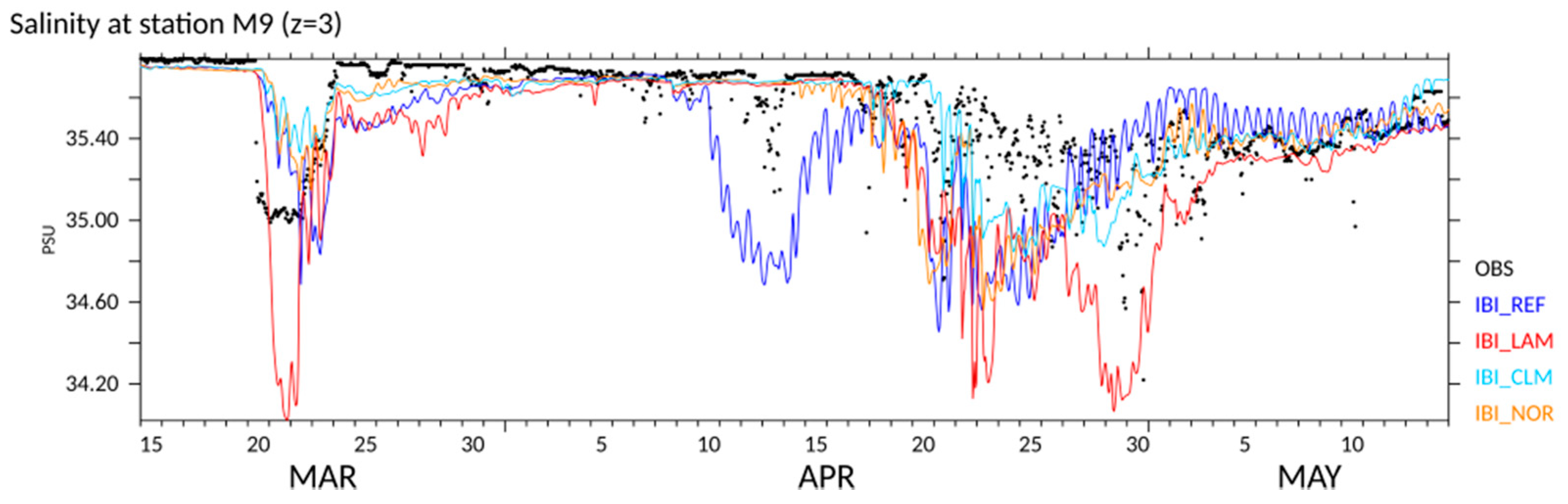
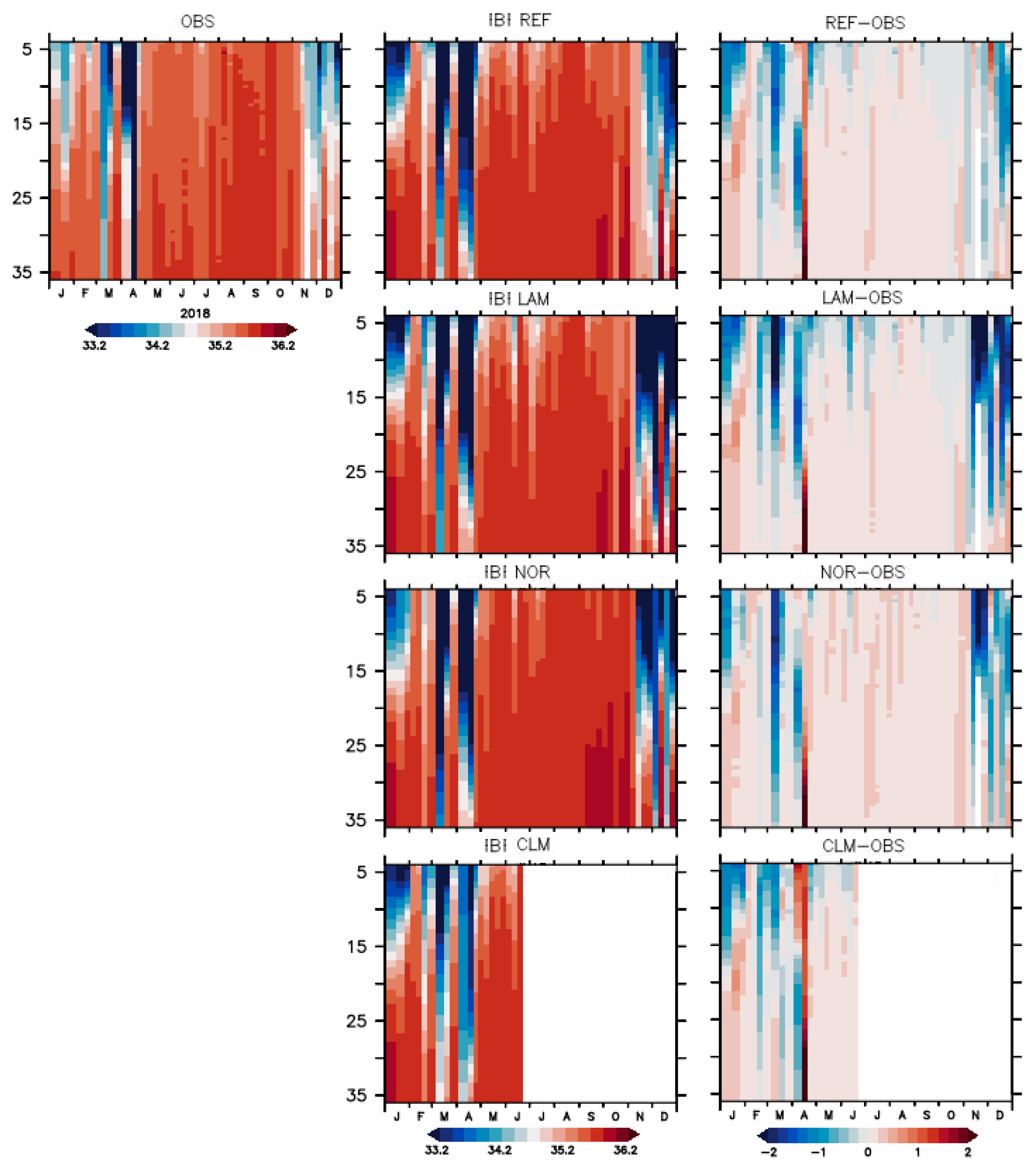
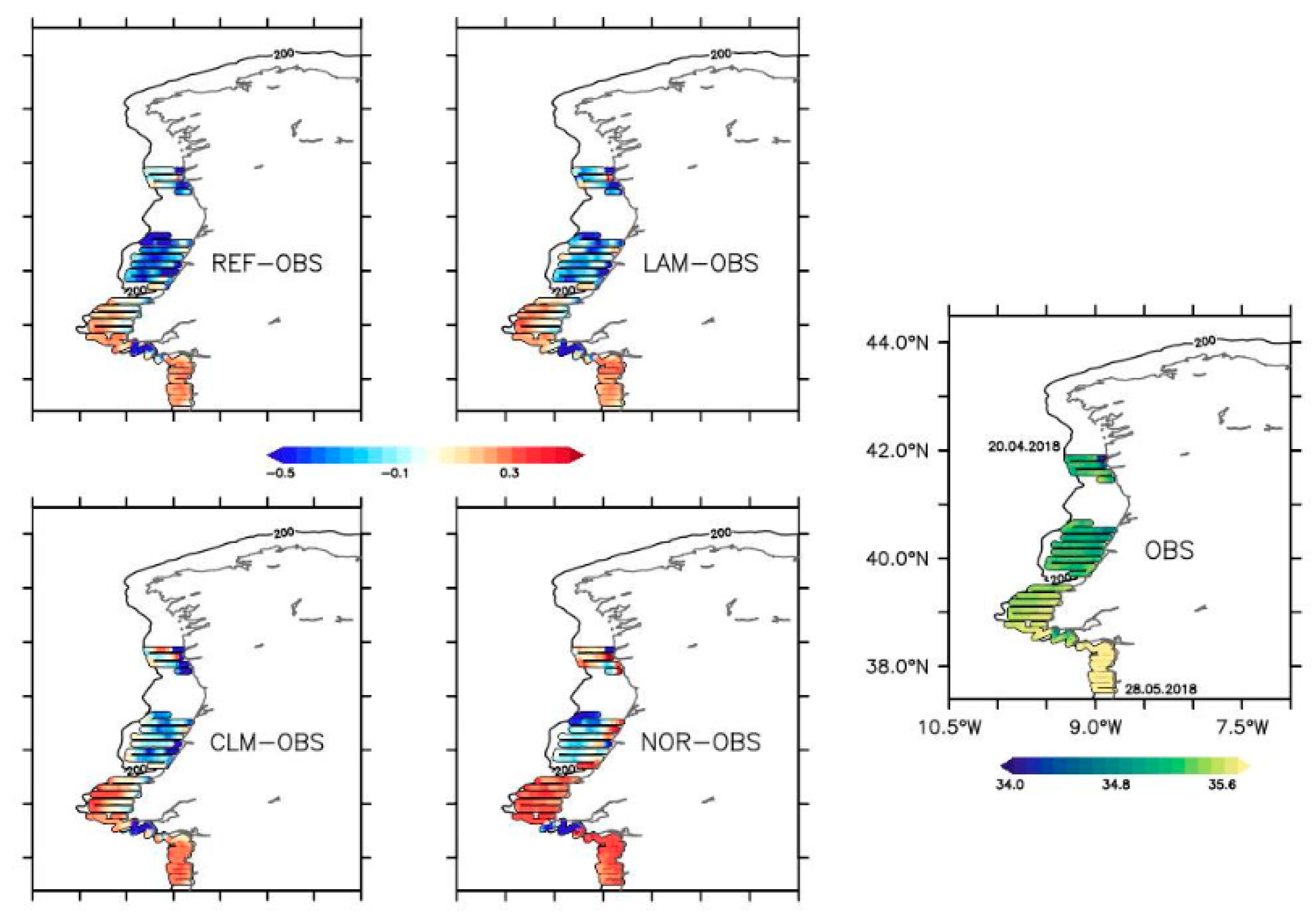
4.8. Impacts in the Western Iberian Shelf

Salinity in the WISHE zone is steadier than in the BISCA area and, as documented in the literature, it is defined by a coastal fresher water mass, usually limited to the narrow shelf, but occasionally extended offshore. The location of the baroclinic front is mainly controlled by the Iberian poleward slope current and its interactions with the shelf waters, resulting in complex front dynamics with occasional episodes marked by strong across-shelf-break advection of lower salinity water masses coming from coastal areas. These intrusions of waters, highly modified by the river and coastal freshwater influence, are clearly identified in the salinity records at mooring sites and they are captured to some extent by the IBI model application (as previously proven through the analysis of the IBI operational performance during the main 2018 observed salinity drops). The IBI model application is adequate to simulate shelf dynamics in ROFI areas of the WISHE zone and the different IBI model scenarios generally reproduce these observed freshwater intrusions, with small variations in timing and/or intensity (with the IBI-NOR and IBI-CLM runs showing better statistical metrics, depending on the buoy). Along the western Galician coast (monitored through the very coastal periodic INTECMAR CTD stations located in front of the Rias), it is the IBI-NOR run, forced with the new LAMBDA river data but without extra coastal runoff, the model scenario that better performs statistically (showing lower RMSE and bias when compared to the INTECMAR 2018 periodic salinity profiles). Emphasize that present IBI model set-up does not include any riverine inflows along this Galician coast, except the Minho and the major, but southern, regional freshwater contributors: the Douro and Mondego rivers. This would mean that salinity budget at this coastal zone off the Rias is rather controlled by the extension of the western Iberian buoyancy plume (mostly fed by freshwater contribution from these three major rivers) than by the local runoff from the nearby Rias itself. Further south, the model scenario assessment performed with the IPMA SSS campaign along the Portuguese shelf shows how all runs feature a similar salinity pattern. This suggests that, in this zone, variations in the imposed river discharge data may not be the main cause of salinity model errors on the shelf freshwater budget. This is so even nearby the Tejo river mouth, where all runs show a similar pattern of salinity differences, pointing out other dynamical factors as more determinant to explain this consistent model behavior.

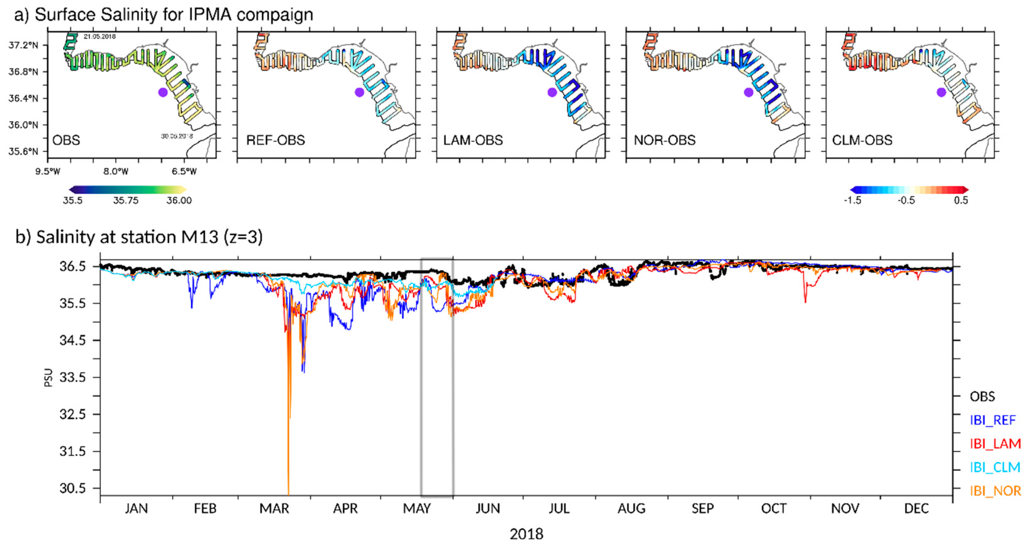
4.9. Impacts in the Gulf of Cadiz

This consistency between model scenarios is also seen in the Gulf of Cadiz. Here, a similar salinity pattern is identified, with main differences between model runs located on-shelf, and especially on coastal areas close to the two rivers considered by IBI (the Guadalquivir and Guadiana) in the CADIZ zone. The occasional comparison with the SSS IPMA campaign (limited to a 9-day campaign in May 2018) indicates an error pattern marked by too-salty modelled waters in the western shelf, getting fresher as moving eastwards closer to the 2 IBI rivers’ mouths. The model run that uses climatological discharges at these two rivers shows lower RMSE and bias values, whereas the 2 runs using LAMBDA inputs (IBI-LAM and IBI-NOR) show higher negative biases. This general anomalously lower model salinity seen in the area for all the runs is directly linked to either the excess of river freshwater contribution imposed at the 2 rivers, especially when using LAMBDA data, or an unrealistic accumulation of freshwater at the river mouths due to the model dynamics. All the nearby on-shelf areas seem affected, as confirmed at the single buoy available in the region (M13, moored offshore at deep waters, but not far from the Guadalquivir mouth).

5. Conclusions and Future Research Directions

In conclusion, the effect of varying imposed river outflows in the IBI operational ocean model system was investigated, showcasing the potential impacts that a new river freshwater model database (such as the LAMBDA one) can have on regional operational forecasts. Some enhancements in model capabilities to better represent salinity and especially baroclinic frontal structures linked to coastal and river freshwater buoyancy plumes have been demonstrated.

Although major impacts were identified on ROFI areas associated with bigger river discharges (i.e., the French shelf in the Gulf of Biscay or the Northwestern Iberian coast), it is found that in some other regions (such as the Portuguese shelf) or in areas with lower riverine freshwater contribution along the study year (such as the Gulf of Cadiz), these impacts related to changes in the imposed river inflows are lower, with other dynamical factors playing a more important role in governing the modelled salinity field.

The CMEMS IBI operational model set-up can reproduce salinity fields with an adequate level of accuracy along the whole water column, including remarkable salinity drop events linked to across shelf water movements that extend river plumes and coastal fresher water zones to more offshore locations at the self-break and beyond. The validation of the 2018 IBI operational solution confirms that the IBI model set-up (and the approach used to include in it the river and coastal fresh water forcing) is valid to achieve realistic simulations of ocean salinity in the IBI area, and they support the decision of using this IBI NEMO model set-up as a base to build the model scenarios proposed here.

The river forcing plays a significant role in the regional simulation of the IBI sea surface salinity, as it is seen when looking at the modelled salinity fields resulting from the different IBI scenario runs. Major impacts are found during spring and summer in the BISCA subregion, when IBI simulations forced by LAMBDA feature fresher water masses on shelf, that extend up to open waters. On the contrary, the simulation forced by a climatology is saltier than the other simulations. The SSS differences between the various simulations are in general more noticeable along the coast and on shelf waters, and especially obvious on the main IBI ROFI areas.

Significant differences in terms of total daily river discharge contributions were identified among the different river flow datasets imposed as freshwater forcing in each sensitivity model run. The use of “realistic” daily updated model-derived river inputs can benefit operational ocean models, especially improving their ability to capture salinity variability, and as demonstrated through the model sensitivity tests performed, their uses can be an option to avoid, or at least to minimize, the use of more static climatological approaches (such as the coastal climatological correction currently applied in the IBI model set-up). Furthermore, some regions, identified here as sensitive to changes in the freshwater forcing data, are of special interest to upgrade their river freshwater contribution, replacing the current freshwater climatological approach. The most noticeable case is the northern Iberian coast, where the current IBI operational model set-up does not count with any river source (with all the regional freshwater contribution coming from the coastal runoff correction applied), despite the existence of numerous small rivers in the area whose cumulated freshwater contribution into the ocean is not negligible (all year round).

A full network of coastal salinity observations would be optimal to evaluate and tune the contribution of freshwater forcing data in ocean simulations. This need of an enhanced in-situ observational coverage should be met for on-shelf and coastal zones (and especially in ROFI areas). Recovered ancillary databases or specific campaigns’ data (such as the RECOPESCA or IPMA data used here) can be useful to study cases, but sustained operational monitoring (i.e., the moored buoys) or routine periodic repetition of salinity observations at specific locations (such as the INTECMAR data) make it possible to analyze the salinity variability. Improvements of satellite-based products are also desired. the with the SMOS products available for coastal uses being mostly reprocessed ones (with an intense use of in-situ observations for calibration and filling gap purposes), again, the in-situ component arises as critical. It should be highlighted that enhancement of the river hydrological observation component is also a key issue: without river flow observations, calibration of hydrological models is limited, decreasing the accuracy of freshwater river flow estimations available to force ocean models.

The progressive replacement of static climatological river inputs in ocean models is likely to become a key research line, needed to upgrade operational ocean circulation models, with a broadening of scope, especially from coastal model services, to increase the number of rivers to be considered as part of the land boundary contribution. This would not be only a matter of including freshwater contribution from major rivers in ocean models (currently the most common approach in operational systems), but also to count with relatively minor ones, which can play a significant role in local coastal dynamics, enhancing its influence under extreme weather event conditions. In that sense, Ruiz-Parrado et al. [70] and Sotillo et al. [71] show how a lack of adequate real-time updated river inputs is a major limitation for the performance of ocean circulation models, including the IBI one, during specific storm events.

Future research lines could include the application of these updated river freshwater model estimations into ocean models, not only in hindcast or analysis mode, but also in forecast runs. The objective would be to substitute the present common approach, mostly based on the use of persistence of the last available river discharge value, by near-real-time updated forecasted river estimations. This upgrade, that can certainly enhance ocean forecast skill, may lead to more integrated multi-disciplinary approaches based on combined near-real-time forecast runs of ocean and hydrological models (both models using the same atmospheric forcing to keep consistency).

References

1. Dai, A.; Trenberth, K.E. Estimates of Freshwater Discharge from Continents: Latitudinal and Seasonal Variations. J. Hydrometeorol. 2002, 3, 660–687. [Google Scholar] [CrossRef] [Green Version]
2. Garvine, R.W.; Whitney, M.M. An estuarine box model of freshwater delivery to the coastal ocean for use in climate models. J. Mar. Res. 2006, 64, 173–194. [Google Scholar] [CrossRef]
3. Fong, D.A.; Geyer, W.R. The Alongshore Transport of Freshwater in a Surface-Trapped River Plume. J. Phys. Oceanogr. 2002, 32, 957–972. [Google Scholar] [CrossRef]
4. Simpson, J.H. Physical processes in the ROFI regime. J. Mar. Syst. 1997, 12, 3–15. [Google Scholar] [CrossRef]
5. Otero, P.; Ruiz-Villarreal, M.; Peliz, A. Variability of river plumes off Northwest Iberia in response to wind events. J. Mar. Syst. 2008. [Google Scholar] [CrossRef]
6. Kourafalou, V.H.; Androulidakis, S.Y. Influence of Mississippi River induced circulation on the Deepwater Horizon oil spill transport. J. Geophys. Res. 2013, 118, 3823–3842. [Google Scholar] [CrossRef]
7. Banas, N.S.; MacCready, P.; Hickey, B.M. The Columbia River plume as cross-shelf exporter and along-coast barrier. Cont. Shelf Res. 2009, 29, 292–301. [Google Scholar] [CrossRef]
8. Santos, A.M.P.; Chícharo, A.; Dos Santos, A.; Moita, T.; Oliveira, P.B.; Peliz, Á.; Ré, P. Physical–biological interactions in the life history of small pelagic fish in the Western Iberia Upwelling Ecosystem. Prog. Oceanogr. 2007, 74, 192–209. [Google Scholar] [CrossRef]
9. Zuo, H.; de Boisséson, E.; Zsoter, E.; Harrigan, S.; de Rosnay, P.; Wetterhall, F.; Prudhomme, C. Benefits of dynamically modelled river discharge input for ocean and coupled atmosphere-land-ocean systems. In Proceedings of the EGU General Assembly, Vienna, Austria, 4–8 May 2020. [Google Scholar] [CrossRef]
10. Bourdalle-Badie, R.; Treguier, A.M. Mercator-Ocean Report. A Climatology of Runoff for the Global Ocean-Ice Model ORCA025; Technical Report MOO-RP-425-365-MER; Mercator Ocean: Toulouse, France, 2006. [Google Scholar]
11. Dai, A.; Qian, T.; Trenberth, K.E.; Milliman, J.D. Changes in Continental Freshwater Discharge from 1948 to 2004. J. Clim. 2008, 22, 2773–2792. [Google Scholar] [CrossRef]
12. Global Runoff Data Centre. Available online: https://www.bafg.de/GRDC/EN/Home/homepage_node.html (accessed on 2 June 2020).
13. Harrigan, S.; Zsoter, E.; Alfieri, L.; Prudhomme, C.; Salamon, P.; Wetterhall, F.; Barnard, C.; Cloke, H.; Pappenberger, F. GloFAS-ERA5 operational global river discharge reanalysis 1979–present. Earth Syst. Sci. Data Discuss 2020. [Google Scholar] [CrossRef]
14. Kourafalou, V.H.; de Mey, P.; Staneva, J.; Ayoub, N.; Barth, A.; Chao, Y.; Cirano, M.; Fiechter, J.; Herzfeld, M.; Kurapov, A.; et al. Coastal Ocean Forecasting: Science foundation and user benefits. J. Oper. Oceanogr. 2015, 8, 147–167. [Google Scholar] [CrossRef]
15. Campuzano, F.; Brito, D.; Juliano, M.; Fernandes, R.; de Pablo, H.; Neves, R. Coupling watersheds, estuaries and regional ocean through numerical modelling for western iberia: A novel methodology. Ocean Dyn. 2016, 66, 1745–1756. [Google Scholar] [CrossRef]
16. Zheng, L.; Weisberg, R.H. Modelling the West Florida Coastal Ocean by Downscaling from the Deep Ocean, Across the Continental Shelf and into the Estuaries. Ocean Model. 2012, 48, 10–29. [Google Scholar] [CrossRef]
17. Lorente, P.; Sotillo, M.; Amo-Baladrón, A.; Aznar, R.; Levier, B.; Sánchez-Garrido, J.C.; Sammartino, S.; de Pascual-Collar, Á.; Reffray, G.; Toledano, C.; et al. Skill assessment of global, regional, and coastal circulation forecast models: Evaluating the benefits of dynamical downscaling in IBI (Iberia–Biscay–Ireland) surface waters. Ocean Sci. 2019, 15, 967–996. [Google Scholar] [CrossRef] [Green Version]
18. Sotillo, M.G.; Cerralbo, P.; Lorente, P.; Grifoll, M.; Espino, M.; Sanchez-Arcilla, A.; Álvarez-Fanjul, E. Coastal ocean forecasting in Spanish ports: The SAMOA operational service. J. Oper. Oceanogr. 2019, 13, 37–54. [Google Scholar] [CrossRef]
19. EU Copernicus Marine Environment Monitoring Service (CMEMS). Available online: https://marine.copernicus.eu/ (accessed on 3 September 2020).
20. Sotillo, M.G.; Cailleau, S.; Lorente, P.; Levier, B.; Aznar, R.; Reffray, G.; Amo-Baladrón, A.; Alvarez-Fanjul, E. The MyOcean IBI ocean forecast and reanalysis systems: Operational products and roadmap to the future Copernicus service. J. Oper. Oceanogr. 2015, 8, 63–79. [Google Scholar] [CrossRef]
21. Le Traon, P.Y.; Reppucci, A.; Fanjul, E.A.; Aouf, L.; Behrens, A.; Belmonte, M.; Bentamy, A.; Bertino, L.; Brando, V.E.; Kreiner, M.B.; et al. From observation to information and users: The Copernicus Marine service perspective. Front. Mar. Sci. 2019, 6, 234. [Google Scholar] [CrossRef] [Green Version]
22. Capet, A.; Fernández, V.; She, J.; Dabrowski, T.; Umgiesser, G.; Staneva, J.; Mészáros, L.; Campuzano, F.; Ursella, L.; Nolan, G.; et al. Operational Modeling Capacity in European Seas—An EuroGOOS Perspective and Recommendations for Improvement. Front. Mar. Sci. 2020, 7, 129. [Google Scholar] [CrossRef] [Green Version]
23. MyCoast Project (EU INTERREG Atlantic Area Transnational Cooperation Programme). Available online: http://www.mycoast-project.org/ (accessed on 3 September 2020).
24. Matulka, A.; Lorente, P.; Sotillo, M.G.; Campuzano, F.; Sobrinho, J.; Taboada, J.; Melo, P.; Ferrer, L.; Robert, M.; Dabrowski, T.; et al. MyCOAST Regional & Coastal Ocean Models. In Proceedings of the 1st MyCOAST Regional Workshop Southeastern Bay of Biscay, San Sebastian, Spain, 11–13 November 2019. [Google Scholar]
25. CMEMS STAC. Copernicus Marine Environment Monitoring Service (CMEMS) Service Evolution Strategy: R&D priorities. Version 3. 2017. Available online: http://marine.copernicus.eu/wp-content/uploads/2017/06/CMEMS-Service_evolution_strategy_RD_priorities_V3-final.pdf (accessed on 3 September 2020).
26. Bronco Project. CMEMS Service Evolution Project. Available online: https://www.mercator-ocean.fr/en/portfolio/bronco-2/ (accessed on 3 September 2020).
27. Lambda Project. CMEMS Service Evolution Project. Available online: http://www.cmems-lambda.eu/ (accessed on 6 April 2021).
28. Pingree, R.D.; Le Cann, B. A shallow meddy (a smeddy) from the secondary Mediterranean salinity maximum. J. Geophys. Res. Ocean. 1993, 98, 20169–20185. [Google Scholar] [CrossRef]
29. Jia, Y. Formation of an Azores Current Due to Mediterranean Overflow in a Modeling Study of the North Atlantic. J. Phys. Oceanogr. 2000, 30, 2342–2358. [Google Scholar] [CrossRef]
30. Carracedo, L.; Gilcoto, M.; Mercier, H.; Pérez, F. Seasonal dynamics in the Azores–Gibraltar Strait region: A climatologically-based study. Prog. Oceanogr. 2014, 122, 116–130. [Google Scholar] [CrossRef] [Green Version]
31. Sánchez, R.F.; Relvas, P. Spring–summer climatological circulation in the upper layer in the region of Cape St. Vincent, Southwest Portugal. ICES J. Mar. Sci. 2003, 60, 1232–1250. [Google Scholar] [CrossRef]
32. Folkard, A.M.; Davies, P.A.; Fiúza, A.F.G.; Ambar, I. Remotely sensed sea surface thermal patterns in the Gulf of Cadiz and the Strait of Gibraltar: Variability, correlations, and relationships with the surface wind field. J. Geophys. Res. Ocean. 1997, 102, 5669–5683. [Google Scholar] [CrossRef]
33. Lobo, F.J.; Le Roy, P.; Mendes, I.; Sahabi, M.; Chiocci, F.L.; Chivas, A.R. (Eds.) Continental Shelves of the World: Their Evolution During the Last Glacio-Eustatic Cycle. 9. The Gulf of Cádiz Continental Shelves; The Geological Society of London: London, UK, 2014. [Google Scholar] [CrossRef]
34. Peliz, Á.; Santos, A.M.P.; Oliveira, P.B.; Dubert, J. Extreme cross-shelf transport induced by eddy interactions southwest of Iberia in winter 2001. Geophys. Res. Lett. 2004, 31. [Google Scholar] [CrossRef]
35. Lobo, F.; Sánchez, R.; González, R.; Dias, J.; Hernández-Molina, F.; Fernández-Salas, L.; del Río, V.D.; Mendes, I. Contrasting styles of the Holocene highstand sedimentation and sediment dispersal systems in the northern shelf of the Gulf of Cadiz. Cont. Shelf Res. 2004, 24, 461–482. [Google Scholar] [CrossRef]
36. González, A.F.; Otero, J.; Guerra, A.; Prego, R.; Rocha, F.J.; Dale, A.W. Distribution of common octopus and common squid paralarvae in a wind-driven upwelling area (Ria of Vigo, northwestern Spain). J. Plankton Res. 2005, 27, 271–277. [Google Scholar] [CrossRef] [Green Version]
37. Haynes, R.; Barton, E.D.; Pilling, I. Development, Persistence, and Variability of Upwelling Filaments off the Atlantic Coast of the Iberian Peninsula. J. Geophys. Res. 1993, 98, 22681–22692. [Google Scholar] [CrossRef] [Green Version]
38. Peliz, A.; Dubert, J.; Santos, A.M.P.; Oliveira, P.B.; Le Cann, B. Winter upper ocean circulation in the Western Iberian Basin—Fronts, Eddies and Poleward Flows: An overview. Deep Sea Res. 2005, 52, 621–646. [Google Scholar] [CrossRef]
39. Kouttsikopoulos, C. Physical processes and hydrological structures related to the Bay of Biscay anchovy. Sci. Mar. 1996, 60, 9–19. [Google Scholar]
40. Kersalé, M.; Marié, L.; Le Cann, B.; Serpette, A.; Lathuilière, C.; Le Boyer, A.; Rubio, A.; Lazure, P. Poleward along-shore current pulses on the inner shelf of the Bay of Biscay. Estuar. Coast. Shelf Sci. 2016, 179, 155–171. [Google Scholar] [CrossRef] [Green Version]
41. Batifoulier, F.; Lazure, P.; Bonneton, P. Poleward coastal jets induced by westerlies in the Bay of Biscay. J. Geophys. Res. Ocean. 2012, 117. [Google Scholar] [CrossRef]
42. Solabarrieta, L.; Rubio, A.; Cárdenas, M.; Castanedo, S.; Esnaola, G.; Méndez, F.; Medina, R.; Ferrer, L. Probabilistic relationships between wind and surface water circulation patterns in the SE of Bay of Biscay. Ocean Dyn. 2015, 65, 1289–1303. [Google Scholar] [CrossRef]
43. Charria, G.; Theethen, S.; Vandermeirsch, F.; Yelekçi, O.; Audriffren, N. Interannual evolution of (sub)mesoscale dynamics in the Bay of Biscay. Ocean Sci. 2017, 13, 777–797. [Google Scholar] [CrossRef] [Green Version]
44. Reverdin, G.; Marié, L.; Lazure, P.; d’Ovidio, F.; Boutin, J.; Testor, P.; Martin, N.; Lourenco, A.; Gaillard, F.; Lavin, A.; et al. Freshwater from the Bay of Biscay shelves in 2009. J. Mar. Syst. 2013, 109–110, S134–S143. [Google Scholar] [CrossRef]
45. Castaing, P.; Froidefond, J.; Lazure, P.; Weber, O.; Prud’homme, R.; Jouanneau, J. Relationship between hydrology and seasonal distribution of suspended sediments on the continental shelf of the Bay of Biscay. Deep Sea Res. Part II Top. Stud. Oceanogr. 1999, 46, 1979–2001. [Google Scholar] [CrossRef]
46. Valencia, V.; Franco, J.; Borja, A.; Fontan, A.; Borja, A.; Collins, M. (Eds.) Oceanography and Marine Environment of the Basque Country Hydrography of the Southeastern Bay of Biscay; Elsevier: Amsterdam, The Netherlands, 2004; Chapter 7; pp. 159–194. [Google Scholar]
47. Ferrer, L.; Fontán, A.; Mader, J.; Chust, G.; Gonzáles, M.; Valencia, V.; Uriarte, A.; Collins, M.B. Low-salinity plumes in the oceanic region of the Basque Country. Cont. Shelf Res. 2009, 29, 970–984. [Google Scholar] [CrossRef]
48. Copernicus Marine In-Situ Tac Data Management Team. Product User Manual for Multiparameter Copernicus In Situ TAC NRT Product (PUM). 2020. Available online: https://archimer.ifremer.fr/doc/00324/43494/ (accessed on 8 April 2021).
49. Venâncio, A.; Montero, P.; Costa, P.; Regueiro, S.; Brands, S.; Taboada, J. An Integrated Perspective of the Operational Forecasting System in Rías Baixas (Galicia, Spain) with Observational Data and End-Users. In Computational Science—ICCS 2019, Lecture Notes in Computer Science; Springer: Cham, Switzerland, 2019; Volume 11539, pp. 229–239. ISBN 978-3-030-22746-3. [Google Scholar]
50. Losada, D.E.; Montero, P.; Brea, D.; Allen-Perkins, S.; Vila, B. Clustering Hydrographic Conditions in Galician Estuaries. In Computational Science—ICCS 2019, Lecture Notes in Computer Science; Springer: Cham, Switzerland, 2019; Volume 11539, pp. 346–360. ISBN 978-3-030-22746-3. [Google Scholar]
51. Szekely, T.; Bezaud, M.; Pouliquen, S.; Reverdin, G.; Charria, G. CORA-IBI, Coriolis Ocean Dataset for Reanalysis for the Ireland-Biscay-Iberia region. SEANOE 2017. [Google Scholar] [CrossRef]
52. Leblond By, E.; Lazure, P.; Laurans, M.; Rioual, C.; Woerther, P.; Quemener, L.; Berthou, P. RECOPESCA: A new example of participative approach to colletc in-situ environmental and fisheries data. Jt. Coriolis Mercator Ocean Q. Newsl. 2010, 37, 40–55. [Google Scholar]
53. Brito, D.; Campuzano, F.J.; Sobrinho, J.; Fernandes, R.; Neves, R. Integrating operational watershed and coastal models for the Iberian Coast: Watershed model implementation—A first approach. Estuar. Coast. Shelf Sci. 2015, 167 Pt A, 138–146. [Google Scholar] [CrossRef]
54. Neves, R. The MOHID concept. In Ocean Modelling for Coastal Management—Case Studies with MOHID; Mateus, M., Neves, R., Eds.; IST Press: Lisbon, Portugal, 2013; pp. 1–11. [Google Scholar]
55. Campuzano, F.; Santos, F.; Ramos de Oliveira, A.I.; Simionesei, L.; Fernandes, R.; Brito, D.; Olmedo, E.; Turiel, A.; Alba, M.; Novellino, A.; et al. Framework for improving land boundary conditions in regional ocean products. In Proceedings of the EGU General Assembly, Vienna, Austria, 4–8 May 2020. [Google Scholar] [CrossRef]
56. Amo, A.; Reffray, G.; Sotillo, M.G.; Aznar, R.; Guihou, K. Product User Manual (PUM) for Atlantic-Iberian Biscay Irish-Ocean Physics Analysis and Forecasting Product: IBI_ANALYSIS_FORECAST_PHYS_005_0012020. Available online: https://resources.marine.copernicus.eu/documents/PUM/CMEMS-IBI-PUM-005-001.pdf (accessed on 3 September 2020).
57. Madec, G. NEMO Ocean General Circulation Model, Reference Manual, Internal Report; LODYC/IPSL: Paris, France, 2008. [Google Scholar]
58. Lellouche, J.-M.; Le Galloudec, O.; Drévillon, M.; Régnier, C.; Greiner, E.; Garric, G.; Ferry, N.; Desportes, C.; Testut, C.-E.; Bricaud, C.; et al. Evalution of global monotoring and forecasting systems at Mercator Océan. Ocean Sci. 2013, 9, 57–81. [Google Scholar] [CrossRef] [Green Version]
59. Chune, S.L.; Nouel, L.; Fernandez, E.; Derval, C.; Tressol, M.; Dussurget, R. Product User Manual (PUM) for GLOBAL Ocean Sea Physical Analysis and Forecasting Products GLOBAL_ANALYSIS_FORECAST_PHY_001_024. 2020. Available online: https://resources.marine.copernicus.eu/documents/PUM/CMEMS-GLO-PUM-001-024.pdf (accessed on 27 October 2020).
60. Carrere, L.; Lyard, F.; Cancet, M.; Guillot, A.; Picot, N. FES 2014, a new tidal model—Validation results and perspectives for 655 improvements. In Proceedings of the ESA Living Planet Conference, Prague, Czech Republic, 9–13 May 2016. [Google Scholar]
61. Aznar, R.; Sotillo, M.G.; Cailleau, S.; Lorente, P.; Levier, B.; Amo-Baladrón, A.; Reffray, G.; Álvarez-Fanjul, E. Strengths and weaknesses of the CMEMS forecasted and reanalyzed solutions for the Iberia–biscay–Ireland (IBI) waters. J. Mar. Syst. 2016, 159, 1–14. [Google Scholar] [CrossRef]
62. Lorente, P.; Sotillo, M.G.; Amo-Baladrón, A.; Aznar, R.; Levier, B.; Aouf, L.; Dabrowski, T.; de Pascual, Á.; Dalphinet, G.R.A.; Toledano, C.; et al. The NARVAL Software Toolbox in Support of Ocean Models Skill Assessment at Regional and Coastal Scales. In Computational Science—ICCS 2019, Lecture Notes in Computer Science; Springer: Cham, Switzerland, 2019; Volume 11539, pp. 315–328. ISBN 978-3-030-22746-3. [Google Scholar] [CrossRef]
63. Olmedo, E.; Martínez, J.; Turiel, A.; Ballabrera-Poy, J.; Portabella, M. Debiased non-Bayesian retrieval: A novel approach to SMOS Sea Surface Salinity. Remote Sens. Environ. 2017, 193, 103–126. [Google Scholar] [CrossRef]
64. Grodsky, S.; Reverdin, G.; Carton, J.; Coles, V. Year to year salinity changes in the Amazon plume: Contrasting 2011 and 2012 Aquarius/SACD and SMOS satellite data. Remote Sens. Environ. 2014, 140, 14–22. [Google Scholar] [CrossRef]
65. Fournier, S.; Lee, T.; Gierach, M. Seasonal and Interannual variations of sea surface salinity associated with Mississippi River plume observed by SMOS and Aquarius. Remote Sens. Environ. 2016, 180, 431–439. [Google Scholar] [CrossRef]
66. Olmedo, E.; González-Haro, C.; Hoareau, N.; Umbert, N.; González-Gambau, V.; Martínez, J.; Gabarró, C.; Turiel, A. Nine years of SMOS Sea Surface Salinity global maps at the Barcelona Expert Center. Earth Syst. Sci. Data Discuss. 2020. [Google Scholar] [CrossRef]
67. Olmedo, E.; González-Gambau, V.; Martínez, J.; González-Haro, C.; Turiel, A.; Portabella, M.; Arias, M.; Sabia, R.; Oliva, R.; Corbella, I. Characterization and Correction of the Latitudinal and Seasonal Bias in BEC SMOS Sea Surface Salinity Maps. In Proceedings of the 2019 IEEE International Geoscience and Remote Sensing Symposium (IGARSS’19), Yokohama, Japan, 28 July–2 August 2019. [Google Scholar] [CrossRef]
68. Campuzano, F. Coupling Watersheds, Estuaries and Regional Seas through Numerical Modelling for Western Iberia. Ph.D. Thesis, Instituto Superior Técnico, Universidade de Lisboa, Lisboa, Portugal, 2018. Available online: http://www.mohid.com/PublicData/products/Thesis/PhD_Francisco_Campuzano.pdf (accessed on 6 April 2021).
69. Sotillo, M.G.; Levier, B.; Lorente, P.; Guihou, K.; Aznar, R.; Amo, A.; Aouf, L.; Ghantous, M. CMEMS Quality Information Document (QUID) for Atlantic-Iberian Biscay Irish-Ocean Physics Analysis and Forecasting Product:IBI_ANALYSISFORECAST_PHYS_005_001. 2020. Available online: https://resources.marine.copernicus.eu/documents/QUID/CMEMS-IBI-QUID-005-001.pdf (accessed on 8 January 2021).
70. Ruiz-Parrado, I.; Genua-Olmedo, A.; Reyes, E.; Mourre, B.; Rotllán, P.; Lorente, P.; García-Sotillo, M.; Tintoré, J. Coastal ocean variability related to the most extreme Ebro River discharge over the last 15 years. Section in Copernicus Marine Service Ocean State Report, Issue 4. J. Oper. Oceanogr. 2020, 13 (Suppl. 1), s160–s165. [Google Scholar] [CrossRef]
71. Sotillo, M.G.; Mourre, B.; Mestres, M.; Lorente, P.; Aznar, R.; García-León, M.; Liste, M.; Santana, A.; Espino, M.; Álvarez, E. Evaluation of the operational CMEMS and coastal downstream ocean forecasting services during the storm Gloria (January 2020). Front. Mar. Sci. 2021, 8, 300. [Google Scholar] [CrossRef]
Figure 1. 2018 Spring (March-April-May) Sea Surface Salinity (SSS) field (psu) simulated by different operational ocean models in the IBI region. The following ocean model solutions, included in the MyCoast Multi-Model Exercise, are shown (each application based on a different model and covering a different geographical domain): The CMEMS IBI regional solution, based on NEMO model and covering the whole IBI region (CMEMS-IBI-NEMO), the Puertos del Estado model (PdE-MITGCM) I for the Strait of Gibraltar (dark blue), the Instituto Superior Tecnico de Lisboa (IST-MOHID) system for the western Iberian domain (purple), the MeteoGalicia (MTG-ROMS) forecast service for the Northwestern Iberian domain (cyan), the Irish Marine Institute (IMI-ROMS) application for Ireland (red), the Service hydrographique et océanographique de la Marine application (SHOM-HyCOM) for the Gulf of Biscay (yellow).
Jmse 09 00401 g001
Figure 2. Study Domain. Location of the in-situ measurements used in this study: fixed moorings (purple), surface transects with thermo-salinometer (blue), coastal profiles with CTD (Conductivity, Temperature, and Depth) instrumentation (orange) and profiles with XBT (eXpendable BathyThermograph) instrumentation (red). Black rectangles show subregions in which the study is focused (IBBIS, CADIZ, WISHE, BISCA). The names of the main rivers included in the IBI model set-up and the geographical features mentioned in the paper are denoted in grey. The shaded field shows the IBI averaged surface salinity over the year 2018, from the reference simulation; the 200 m isobath, delimiting the shelf, is depicted in dashed line.
Jmse 09 00401 g002
Figure 3. Average daily freshwater discharges imposed as forcing in different IBI sensitivity runs in (a) IBBIS, (b) BISCA, (c) WISHE and (d) CADIZ areas, in 2018. The freshwater forcing FWF_REF, FWF_LAM, FWF_CLM and FWF_CRF data sources are respectively depicted in blue, red, dashed blue and grey.
Jmse 09 00401 g003
Figure 4. 2018 yearly averaged maps of sea surface salinity (SSS) simulated by CMEMS IBI (a) and derived from remotely sensed SMOS data (b). Monthly maps (March 2018) of skill metrics derived from the comparison of entire salinity profiles observed by Argo floats and modelled by CMEMS IBI: root mean squared error (c) and correlation (d). Daily salinity profiles collected by Argo floats (e) and IBI (f) in the Gulf of Biscay (BISCA zone) during March 2018. Averaged profiles exposed in solid black lines. Mean depth values gathered in blue.
Jmse 09 00401 g004
Figure 5. (a) Contingency table focused on significant sea surface salinity (SSS) drops detected during 2018 at coastal buoys moored around the Iberian Peninsula (buoys M2–M12 used, see Figure 2 for location). Hit, miss and false alarm events are highlighted in green, purple and yellow colors, respectively. (b) Six-month observed (blue dots) and IBI modeled (red line) SSS timeseries at Silleiro buoy (M12). Relevant SSS drops marked with colored dashed squares. (c) Three-month timeseries comparison of SSS observed at Cabo de Peñas buoy (M7) and modelled by CMEMS-IBI at the closest grid point.
Jmse 09 00401 g005
Figure 6. (a) Seasonal surface salinity in winter 2018 from IBI_REF (left panel) and difference of seasonal surface salinity between IBI_LAM, IBI_NOR, IBI_CLM (respectively in panels from left to right) and IBI_REF. (b) Same as (a) but in spring. (c) Same as (a) but in summer. (d) Same as (a) but in autumn. Red (blue) shading in the panels (a) to (c) means that the simulation is saltier (fresher) than IBI_REF. Salinity mean values and statistical metrics (root mean square error and bias computed when comparing each scenario with the reference one) are shown in each panel. Grey dots show the river mouth locations of the rivers considered in the IBI model set-up.
Jmse 09 00401 g006
Figure 7. (a) Taylor diagrams showing observed-modelled salinity comparisons at moorings in the BISCA, WISHE and CADIZ areas. Each location is represented by a different symbol, whereas colors represent the model scenario simulation (IBI_REF in blue, IBI_CLM in light blue, IBI_LAM in red and IBI_NOR in orange). M3, M4 and M10, because of the important bias between observations and simulations, are not represented here. (b) Timeseries of salinity at station M6, at the shelf-break of Santander, Northern Spain, in BISCA. The color code is the same as in panel (a).
Jmse 09 00401 g007
Figure 8. Sea surface salinity (SSS) measured with XBTs from the RECOPESCA campaign for May 2018 in the BISCA area. The right panel shows observed (OBS) salinity, whereas panels on the left show the respective differences between the simulated salinity by each model scenario (i.e., IBI_REF, IBI_LAM, IBI_CLM, IBI_NOR) and the RECOPESCA observations.
Jmse 09 00401 g008
Figure 9. Timeseries of salinity at mooring station M9, at the shelf-break of Northwestern Iberia, from 15 March to 15 May 2018. Observed salinity represented by black dots and the different IBI model scenarios by solid lines (IBI_REF in blue, IBI_CLM in light blue, IBI_LAM in red and IBI_NOR in orange color).
Jmse 09 00401 g009
Figure 10. Salinity profiles measured by CTD at the INTECMAR station C3 (8.96° W/42.48° N) for 2018 in WISHE area (left panel) in comparison with salinity profiles simulated, at the closest model grid point, by the different model scenarios—IBI_REF, IBI_LAM, IBI_NOR and IBI_CLM (middle panel). Differences between modelled and observed salinity profiles (right panels). Note that IBI_CLM run is shorter than other simulations.
Jmse 09 00401 g010
Figure 11. Surface salinity during the IPMA campaign in May 2018 in WISHE area. The right panel shows observed (OBS) salinity (measured by means of a thermo-salinometer), whereas panels on the left show the respective differences between the simulated salinity (from each model scenario: i.e., IBI_REF, IBI_LAM, IBI_CLM, IBI_NOR) and the IPMA observations.
Jmse 09 00401 g011
Figure 12. (a) Surface salinity during the IPMA campaign in late May 2018 in the CADIZ area. The left panel shows the observed salinity measured (by means of a thermo-salinometer), and the other panels (from left to right) show differences between modelled salinities (from IBI_REF, IBI_LAM, IBI_NOR, IBI_CLM model scenarios) and the observations. The purple dot depicts the location of the mooring buoy M13. (b) Timeseries of salinity at station M13, at the shelf-break of the Gulf of Cadiz. Observed salinity is represented by black dots and the different IBI model scenarios by solid lines (IBI_REF in blue, IBI_CLM in light blue, IBI_LAM in red and IBI_NOR in orange color). The grey rectangle highlights the period of the IPMA campaign in the Gulf of Cadiz.
Jmse 09 00401 g012