Article

A Regional Operational Model for the North East Atlantic: Model Configuration and Validation

1
Marine Institute, Rinville, Oranmore, Co Galway, Galway, Ireland
2
Oceanography Department, Alexandria University, Alexandria 21500, Egypt
3
The Numerics Warehouse Ltd. Tyrone, Kilcolgan, Co. Galway, Galway, Ireland
*
Author to whom correspondence should be addressed.
J. Mar. Sci. Eng. 2020, 8(9), 673; https://doi.org/10.3390/jmse8090673
Submission received: 15 July 2020 / Revised: 26 August 2020 / Accepted: 27 August 2020 / Published: 1 September 2020
(This article belongs to the Special Issue Ocean Modelling in Support of Operational Ocean and Coastal Services)

Abstract

:
An operational model for an area of the northeast Atlantic that encompasses all of Ireland’s territorial waters has been developed. The model is an implementation of the Regional Ocean Modelling System (ROMS) and uses operationally available atmospheric and boundary forcing, and a global tide solution for tidal forcing. River forcing is provided by climatological daily discharge rates for 29 rivers across Ireland, west Britain, and west France. It is run in an operational framework to produce 7-day hindcasts once a week, and daily 3-day forecasts which are published in a number of formats. We evaluated the model skill by comparing with measured data and calculating statistics such as mean error, root mean square error (RMSE), and correlation coefficient. The observations consist of satellite Sea Surface Temperature (SST), total surface velocity fields from satellite, water level time series from around the Irish coast, and temperature and salinity data from Array for Real-Time Geostrophic Oceanography (ARGO) and Conductivity Temperature Depth (CTD) profiles. The validation period is from 1 January 2016 until 31 December 2019. The correlation coefficient between the model and satellite SST is 0.97 and recorded in March and April 2018. The model error is about 5% of the total M2 amplitude in the Celtic Sea recorded at Dunmore East tide gauge station. The maximum RMSE between the model and the CTD temperature profiles is 0.8 °C while it is 0.17 PSU for salinity. The model correctly defines the shelf water masses around Ireland. In 2019 the Irish Coastal Current (ICC) was very strong and well defined along most of the western Irish coast. The model results have well reproduced the ICC front for the whole simulation period.

1. Introduction

Ireland is located in a hydrographically interesting part of the northeast Atlantic Ocean where the regimes of the deep ocean and the continental shelf interact. The North Atlantic Current (NAC) divides southwest of the Rockall Bank and produces several branches flowing roughly to the northeast or southeast [1]. The Rockall Trough is one pathway by which heat is transported into the Nordic Seas [2,3] (see Figure 1). The continental shelf edge has a poleward current associated with it, which is seasonally variable [4,5,6] and is the interface for the ocean-shelf exchange of nutrients and carbon [7]. On the Irish shelf, the Irish Shelf Front (ISF) separates fresher Irish coastal waters from the oceanic Eastern North Atlantic Water (ENAW) at ca. 11° W [8]. The Shannon River on the west coast of Ireland is the largest river in the region with a mean annual discharge of 186 m3 s−1 [9], but there are also significant freshwater discharges from rivers on the south coast of Ireland and west coast of Britain as well as from further afield such as the Loire in France. This induces vertical density stratification on the shelf while thermal stratification is an important process during the summer months. In contrast, mixing due to tide and wind creates areas with well-mixed water, such as the Irish Sea. Fronts occur between these stratified and well-mixed areas, such as the Celtic Sea front, which is located at the southern entrance to the Irish Sea [10]. A seasonal density-driven current, the Irish Coastal Current (ICC) has been described by [10,11]. The ICC is linking Land’s End in southwest England to the northwest coast of Ireland and this may provide an important pathway for harmful phytoplankton, which has significant consequences for the aquaculture industry on the west coast of Ireland and onwards to the coast of west Scotland. The Scottish Coastal Current flows northwards from the Irish Sea along the west coast of Scotland [12].
Operational modelling of physical ocean fields has developed rapidly over the last decade in response to the needs of the marine community. The availability of hindcasts and forecasts of the hydrodynamic properties for specific regions is of great benefit to decision makers in areas such as marine environmental management, and the aquaculture and fisheries industries. Operational models that forecast the physical state of the oceans exist for European oceans (e.g., [13,14,15,16,17,18,19,20,21,22,23,24,25,26,27]). The first operational models developed in Ireland and described by [15,16].
Ref. [24] described an operational biogeochemical model for the North East Atlantic Ocean region. The model domain covered a significant portion of the North-West European continental shelf with a horizontal and vertical resolution of ≈4 km and 40 sigma levels, respectively. It was one-way nested within the high resolution (1/12°) CMEMS Ocean (http://www.CMEMS-ocean.fr) PSY2V4R2 operational model of the North Atlantic whereby daily values for potential temperature, sea surface height and velocity are linearly interpolated at the open ocean boundaries. A simple nitrogen-based NPZD model developed described in [28] was dynamically coupled to ROMS. The model has successfully represented the intra-annual variability of surface chlorophyll and nitrate concentrations at monthly time scales.
There have already been several studies simulating the North Atlantic region including [27,29,30,31,32,33,34,35,36]. Overall, properly validated hydrodynamic models can provide information on the present and near-future states of ocean systems, which is of value to a wide range of users from both the private sector and the general public.

Objectives of the Study

This study presents the set-up and results from the validation of a high-resolution numerical operational model (hereafter called NEA_ROMS) developed at Irish Marine Institute. Validation of NEA_ROMS was carried out for the time period from January 2016 until December 2019 using observational data from various sources. The model has been compared with satellite SST, tide gauges, Argo, and CTD temperature and salinity profiles. In addition, the Geostrophic and Ekman Current Observatory GEKCO surface data was used to validate model velocity fields. Additionally, this study will focus on the Irish coastal waters and the authors will examine the representation of the Irish coastal current (ICC) in the model. Section 2 describes the model implementation, and nesting procedures, Section 3 presents the validation against observational data, Section 4 describes the model results related to the ICC, and Section 5 provides the discussion and conclusions.

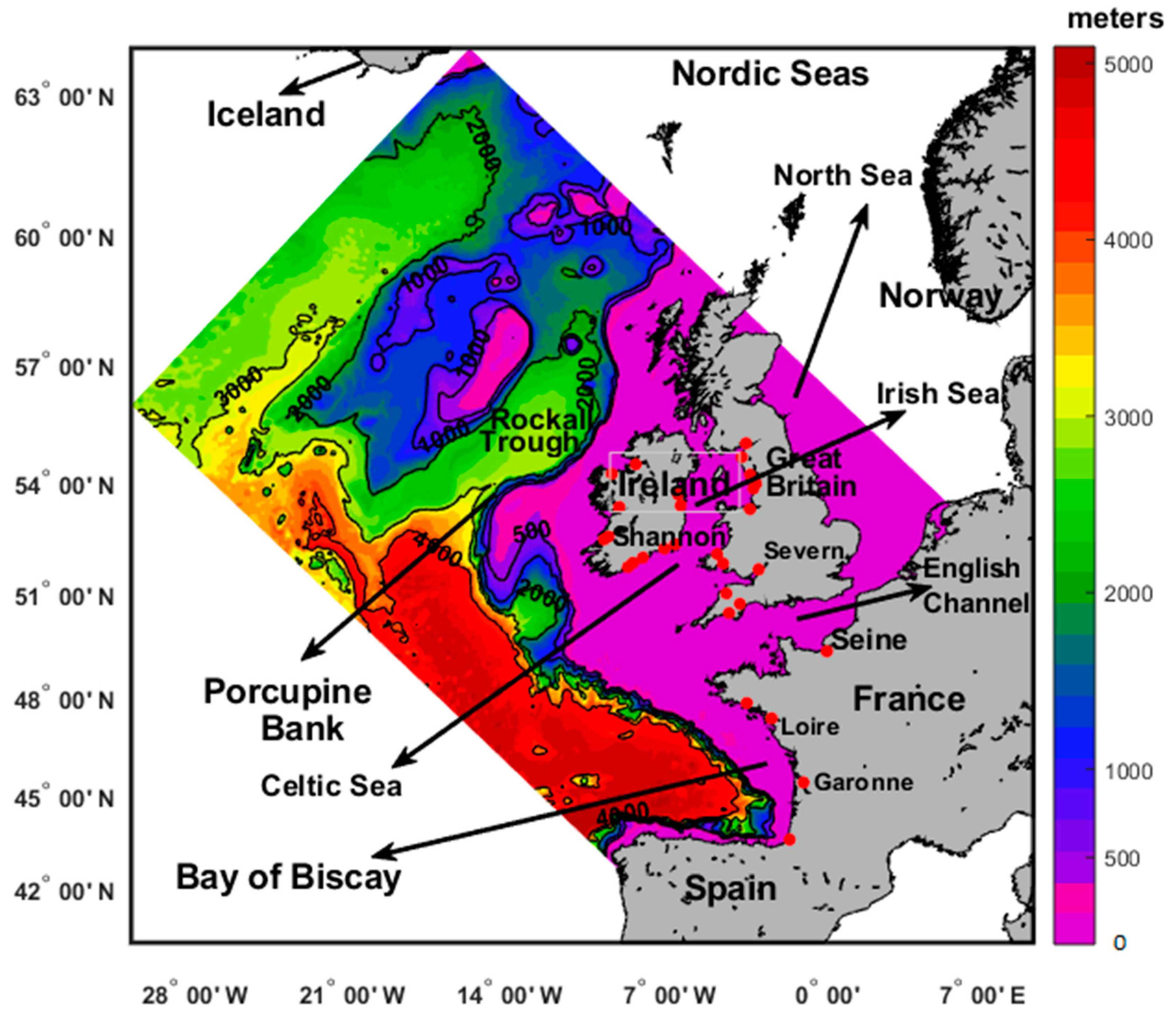
2. Model Design and Implementation

The model used in this study is an implementation of the Regional Ocean-Modelling System (ROMS). ROMS has been proven to demonstrate substantial skill in forecasting [37] and has been used in a number of successful operational systems [38,39,40]. ROMS is a primitive-equation, free-surface, hydrostatic model as described in [41]. In the horizontal, it uses orthogonal curvilinear coordinates on an Arakawa “C” grid while utilizing a terrain-following (sigma) coordinate in the vertical. The momentum equations are solved using a split-explicit time-stepping scheme whereby a whole number of barotropic time steps are carried out within each baroclinic time step to solve the barotropic momentum equations. The prognostic variables of the model are surface elevation, potential temperature, salinity, and velocity. All the model equations are written in rectangular coordinates and contain spatially and temporally varying horizontal eddy viscosity and diffusion coefficients. Vertical diffusion is calculated using the K-profile parameterization (KPP) [42] and a modified Jacobian method [43] is used to calculate horizontal pressure-gradient forces. The associated parameters with KPP vertical turbulent closure scheme have been enhanced to tune the vertical profile of currents, temperature, and salinity by [44,45,46,47]. Recursive MPDATA is used for the advection of tracers [48]. Bottom stress is applied using the logarithmic “law of the wall” with a constant roughness length of 0.01 m.
The NEA_ROMS model domain covers a significant portion of the North-West European continental shelf and also the Porcupine and Rockall Banks and the Rockall Trough as shown in Figure 1. NEA_ROMS model has a horizontal resolution of 1.1 km and 40 vertical sigma levels with the highest concentration of levels at the surface and the bottom. The basin-scale daily average lateral boundary conditions are provided from the high resolution (1/12°) CMEMS_GLOBAL_ ANALYSIS_ FORECAST_ PHY _001_024 model [49]. The daily values are for potential temperature, salinity, sea surface height, and velocity components at the three open boundaries. The discharges from 29 rivers are included in the NEA_ROMS model. The rivers comprise the major rivers of Ireland, west Britain, and west France, as well as some more minor Irish rivers. The discharge rates are average daily values calculated from many years of historical discharge data for 29 rivers across Ireland, west Britain, and west France. Furthermore, the nested model temperature and salinity fields were nudged toward the GLOBAL_ ANALYSIS_ FORECAST_ PHY _001_024 operational model. Within the NEA_ROMS, several one-way nested shelf models have been implemented to downscale and forecast near the Irish coasts.
The model bathymetry utilizes data from a number of sources. Large-scale multi-beam mapping of Irish territorial waters has been carried out under the Irish National Seabed Survey (INSS) and the Integrated Mapping for the Sustainable Development of Ireland’s Marine Resource (INFOMAR) programs. These datasets along with an extensive single-beam archive maintained by the Marine Institute were used to develop the model bathymetry. A 1 × 1 km Celtic Sea bathymetry [50] complements the bathymetry in the Irish and Celtic Seas while GEBCO data is used for the bathymetry in non-Irish waters. The model minimum depth is set at 10 m near the coastline. In order to reduce the pressure gradient errors, we smoothed the model bathymetry according to the rx0 factor of Beckman and Haidvogiel [51,52].

2.1. Lateral Boundary Conditions

The model has three open boundaries in the North, East, and West. The NEA-ROMS lateral boundary conditions are taken from the CMEMS GLOBAL_ANALYSIS_FORECAST_ PHY _001_024 at 50 vertical levels are ranging from 0 to 5500 m. The CMEMS model is version 3.1 of NEMO [49]. The model data is freely available via the Copernicus Marine Environment Monitoring Service (CMEMS) web site marine.copernicus.eu. The analysis is updated weekly while a 10-day forecast is updated daily. The model boundary parameters are temperature, salinity, total velocity components, surface elevation, and barotropic velocity components. The nesting was designed to ensure that the volume transport across the open boundary of the nested model matches the volume transport of the CMEMS global model.
For the barotropic velocity, we used the scheme proposed by [53]. At the outflow, we impose
φ n nested ¯ = [ g H nested ( η nested η nesting ) ] φ n nested ¯ H nesting + η nesting H nested + η nested
where φ n ¯ = 1 H + η H η φ n dz is the normal barotropic velocity at the open boundaries and g the gravity, while at the inflow will be φ n nesting ¯ = φ n nested ¯
For the baroclinic velocity, we impose the normal velocity according to the following formula:
n 2 n 1 H nested η nested φ n nested dzdn = n 2 n 1 H nesting η nesting φ n nesting dzdn
where φ n is the normal component to the three open boundaries in m/s. For the temperature and salinity, we used a third-order upstream scheme with implicit mixing for horizontal advection [54]. Whenever the normal velocity is directed outwards:
T nested t + φ n nested T nested y = 0 ; S nested t + φ n nested S nested y = 0
While on the inflow the temperature and salinity are prescribed to be identical to that interpolated to CMEMS global model values. Where n1, n2 are the extremes of the open boundary section, ηnesting, and Hnesting are the surface elevation and the bathymetry of the nested model, while ηnested and Hnested are the surface elevation and bathymetry of the CMEMS global model and φ n is the normal velocity component to the open boundaries. The total tangential velocity at the open boundaries is set to be equal between the CMEMS global model and the nested model.
The nested model temperature and salinity fields were nudged toward the CMEMS global model values in the right-hand side (r.h.s) of the prognostic fields following [55]. Indicating temperature or salinity with ‘gamma’ we add a relaxation term such as:
γ t = r . h . s   1 Γ ( γ γ CMEMS )
Here Γ is the relaxation time that varies smoothly from 20 model grid internal points to the open boundaries with values of 240 s to 100 days. This nudging prevents a substantial model drift from the CMEMS global model values.
Finally, the tidal forcing is prescribed at the model boundaries by applying elevations and barotropic velocities for 10 major tide constituents (M2, S2, N2, K2, K1, O1, P1, Q1, Mf, Mm) which are obtained from the TPXO8 global inverse barotropic tide model [56]. Radiation conditions are specified at the boundaries for depth-averaged velocity after [53] and also for water level after [57]. Radiation conditions are prescribed for tracers and baroclinic momentum [55].

2.2. Surface Boundary Conditions

The atmospheric data for the computation of the surface forcing are taken from the global high resolution (0.125°) atmospheric model run by the European Centre for Medium Range Weather Forecasts (ECMWF) with 3-hourly temporal step. This has changed in 2019 to hourly fields with spatial resolution (0.1°). The atmospheric fields used are air temperature, relative humidity, wind velocity at 10 m above sea level, mean sea level pressure, cloud cover, total precipitation, and solar radiation (net surface and longwave radiation). In order to parametrize the air–sea interaction processes, the wind stress, heat fluxes, and evaporation rate are computed by means of interactive bulk formulae making use of atmospheric data and the model predicted sea surface temperature according to [58]. The NEA-ROMS heat fluxes are computed interactively according to [13] and described in [59] the heat flux boundary condition is given by
ρ o C P K H T z | z = η = Q T   + Q T   ( SST CMEMS SST m )
where QT is the total net heat flux according to the formula:
QT = QS − Qb − Qe − Qh
The last term in Equation (5) is the heat flux correction term. ∂Q/∂T is the heat flux correction. which is set at 80 W·m−2·°C−1 for NEA-ROMS. SSTm is the model sea surface temperature and salinity and SSTCMEMS is the reference SST. QS, Qe, Qb, and Qh are the short, latent, back, and sensible heat fluxes in W/m2. (KH) is the vertical mixing coefficients for tracers in (m2·s−1). This heat flux correction, which was extracted from CMEMS, sea surface temperature, is to control the simulation from drifting away from the CMEMS values.
The momentum flux boundary condition for the surface takes the form:
ρ o K M ( u , v ) z | z = η = ( τ wx , τ wy )
In Equation (7), η is the free surface elevation in (m) and τwx, τwy are the wind stress components in Nm−2 calculated from the equation
τ = CD ρa |W|* W
where ρa = 1.2 kg·m−3 is the density of air, CD is the drag coefficient in Equation (8) computed according to [60]. While (W) is the wind speed component and (KM) is the vertical mixing coefficient for momentum expressed in m2·s−1.
Daily averaged freshwater discharges were specified for a total of 29 rivers across Ireland, west Britain, and west France. The climatological mean river discharge values were obtained from various sources (Table 1), and the location of each river is shown in Figure 1. The NEA_ROMS rivers salinity was set to zero and the river temperatures were not prescribed. Discharge rates for the Irish rivers were obtained from the Office of Public Works (OPW) http://www.opw.ie/ and Electricity Supply Board (ESB) databases. The NEA_ROMS operational river discharge system is evolving. In 2019 our team managed to implement near real time flow rates for Corrib River obtained from OPW. The Corrib River is located inside Galway Bay on the west coast of Ireland. UK rivers data were downloaded from the Centre for Ecology and Hydrology website (https://www.ceh.ac.uk/our-science/projects/national-river-flow-archive). Data from the French rivers were provided from the national database “HYDRO”, run by the French ministry of ecology and solidarity transition. The corresponding model salt flux boundary condition is given according to [61]:
K H S z | z = η = SSS ( E - P - ( R A ) )
where E is the evaporation, P the precipitation, R is the Rivers climatological daily discharge, A is mouth cross-section in m2, and SSS in Equation (8) represents the sea surface model salinity.

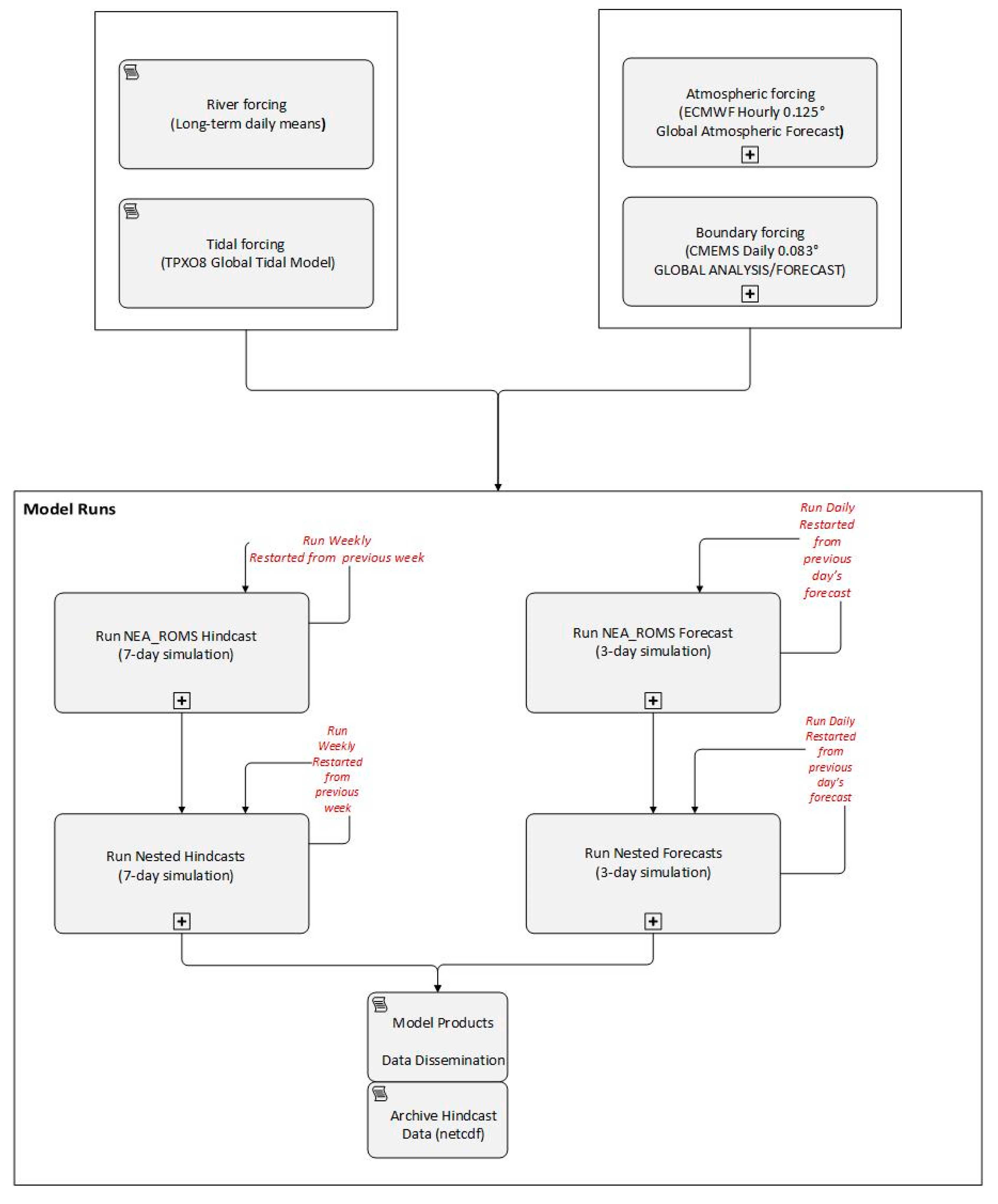
2.3. Operational Setup

Figure 2 describes the schematic of the NEA_ROMS operational functioning during the simulation period. At the beginning of each year, a new NEA-ROMS run is initialized using interpolated fields from the CMEMS Ocean global model. Tide and river forcing files are created to provide forcing data for the full year ahead. The NEA_ROMS model is then run in hindcast/forecast mode for the year. This entails accessing the CMEMS Ocean weekly analysis run to provide boundary data for the NEA-ROMS hindcast run, while the latest CMEMS Ocean forecast data is used for our forecast boundary forcing. Similarly, the latest ECMWF forecasts are used for atmospheric forcing. The 7-day hindcast is initialized using a restart file from the end of the previous 7-day hindcast. The final output file of the hindcast is used to initialize the first forecast of the current week. A 3-day forecast is created every day using a restart file from the previous forecast to initialize the run. NEA_ROMS state variables (i.e., temperature, salinity, sea surface height, barotropic and baroclinic velocity fields) are saved to netCDF files in hourly snapshots. Selected points in the domain have data saved at the higher frequency of 10 min for use in model validation and also to provide boundary data for two high-resolution coastal models which are also part of the operational system. Model results are published on the Marine Institute website http://www.marine.ie/Home/site-area/data-services/marine-forecasts/marine-forecasts. A rolling month of model output is published to the Marine Institute THREDDS http://milas.marine.ie/thredds/catalog.html and ERDDAP https://erddap.marine.ie/erddap/index.html servers. Monthly mean fields of some parameters (e.g., surface and bottom temperature) are also published to these servers.

2.4. Observations Data and Methods of Analysis

Data used to validate the NEA-ROMS include Sea Surface Temperature (SST) from satellites, tide gauges, ARGO floats, and CTD salinity and temperature profiles.
The satellite SST product used is the European North West Shelf/Iberia Biscay Irish Seas High Resolution ODYSSEA L4 Sea Surface Temperature Analysis dataset which is available for download from the CMEMS website (data product, SST_ATL_SST_L4_NRT_OBSERVATIONS_010_025). The product consists of daily averaged SST values. The data valid for a particular day (from previous day 12:00 to current day 12:00) at a horizontal resolution of 0.02° × 0.02° for a domain covering the European North West Shelf and Iberia-Biscay-Irish Seas. It is a multi-sensor Level 4 analysis which aims to provide an estimate of the night time SST based on original SST observations http://resources.marine.copernicus.eu/documents/QUID/CMEMS-SST-QUID-010-025.pdf. The data from 1 June 2019 were replaced by ODYSSEA product, SST_NWS_SST_L4_NRT_OBSERVATIONS_010_003, https://cmems-resources.cls.fr/documents/PUM/CMEMS-OSI-PUM-010-003-010.pdf.
The authors validated NEA_ROMS Sea Surface Height (SSH) using observed time series from tide gauges around the Irish coast (Irish National Tide Gauge Network) https://data.gov.ie/dataset/irish-national-tide-gauge-network. The sampling frequency of the measured tide data ranged from 5 to 15 min while the model output is produced at a frequency of 10 min. Harmonic analysis was carried out on the observed and modelled time series using the T-TIDE software in MATLAB [62]. In addition, the surge component was calculated following [62], for observed and modelled data at the locations of Irish tide gauges, and the difference statistics are presented. According to [63], the surge (residual) component of sea level is defined as the total water level minus the tide.
Sea level elevation = predicted tide level + storm surge height
In this study, ARGO float profiles were used to validate the NEA_ROMS temperature and salinity fields. Drifting ARGO floats record vertical profiles of temperature and salinity in the upper 2000 m of the ocean approximately every 10 days and transmit the data via the ARGO satellite system to a number of data processing centers [64,65,66,67]. The data is then made freely available via public access site http://www.argo.ucsd.edu/. Irish Marine Institute (IMI) have used only ARGO data in delayed mode. For the corresponding modelled profile, the authors used the hourly snapshots model output file corresponding to the date the ARGO profile was acquired, and the grid point closest in location to the ARGO profile. The ARGO temperature and salinity were then interpolated onto the modelled vertical profile for that grid point. The authors chose the year 2019 as one that has the best ARGO tracks coverage for the south of the Porcupine Bank, the southern and northern entrance to the Rockall Trough area.
The IMI maintains an archive of all Conductivity Temperature Depth (CTD) measurements taken from the research vessels operated by the Institute. During the period of January 2016 to December 2019, CTDs were acquired from the research vessels in the shelf seas around Ireland with the highest frequency in the months of spring and summer. The authors chose the year 2017 as one that provides the best Irish shelf waters coverage. These data are analyzed to assess the model performance in the shallow, coastal waters around Ireland.
In the study, the authors used the Geostrophic and Ekman Current Observatory GEKCO surface data to validate model velocity fields and Eddy Kinetic Energy (EKE), then compare it with CMEMS Ocean global model (EKE). The data are daily averages 0.25° spatial resolution obtained from Mean Absolute Dynamic Topography (MADT) at the gridded DUACS products. The DUACS system has been producing, as part of the CNES/SALP project, and the Copernicus Marine Environment and Monitoring Service (CMEMS), high quality multi-mission altimetry Sea Level products for oceanographic applications, climate forecasting centers, geophysics and biology communities http://www.aviso.altimetry.fr [68,69]. The geostrophic velocity anomalies presented in this study were deduced from MADT maps with geostrophic approximation as follows:
For NEA_ROMS domain, the mean velocity U ¯ g , V ¯ g in the x and y directions and the anomalies   U g   , V g from the mean were computed
U g   =   g f h y , V g = g f h x
where h is the absolute dynamic topography anomaly in meters, g is the gravity acceleration in m/s2 and f = 2Ω sin ϕ, where Ω = 2π/T is the earth angular velocity in s−1, T is the earth periodic time = 86,400 s (1 day in seconds), and ϕ is the latitude in degrees. The variance of these velocity anomalies was considered as Eddy Kinetic Energy (EKE), representative of mesoscale activity.
EKE   =     1 2   ( U g 2 + V g 2 )
Model velocities were taken daily at the first sigma layer to compute EKENEA_ROMS to be exactly like EKEGEKCO and EKECMEMS between 1 January 2017 and 31 December 2017. Velocity time series were subsampled at a daily period of GEKCO MADT as described in [70]. Space and time dependent EKEGEKCO and EKENEA_ROMS fields were eventually averaged temporally to produce mean EKE fields.

3. Validation of NEA_ROMS Results against Observations

In this part, the authors will validate and discuss the NEA_ROMS results against available observations described previously in Section 2.4.

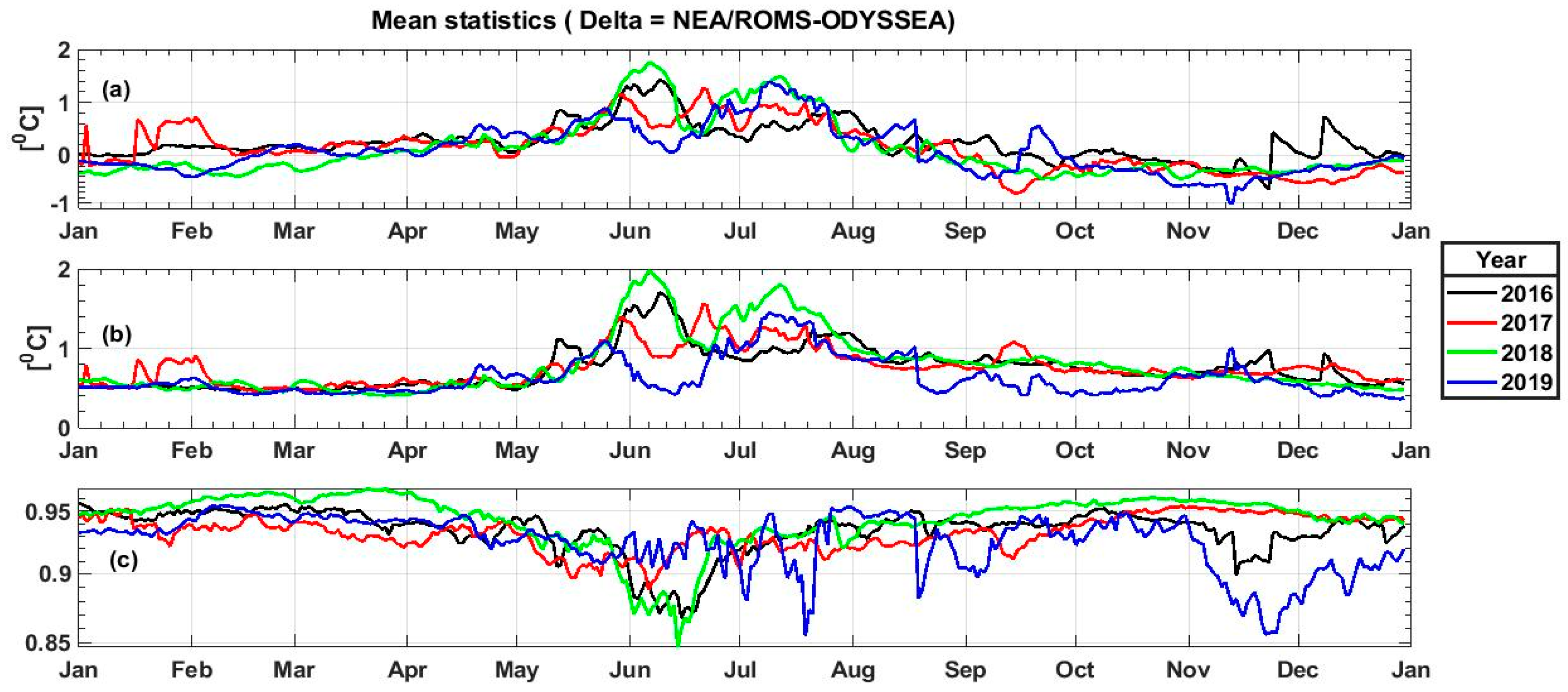
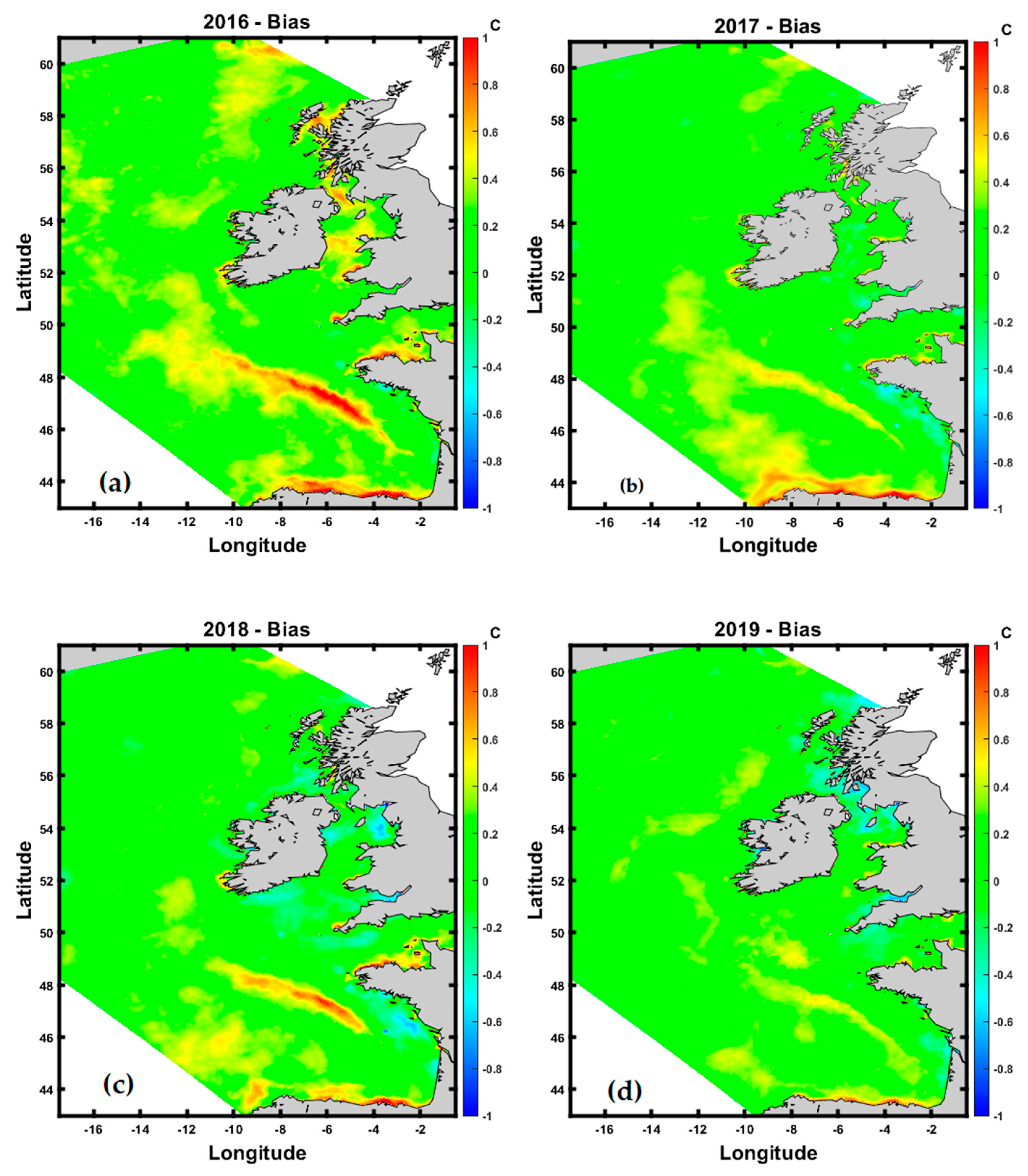
3.1. Comparison between NEA_ROMS and ODYSSEA SST during the Simulation Period

Figure 3a–c shows the temporal evolution of the daily mean SST basin averaged statistics for the NEA_ROMS Model-ODYSSEA satellite data for the whole model simulation period from 1 January 2016 until 31 December 2019 in °C. The daily SST bias between the NEA_ROMS and ODYSSEA satellite is shown in Figure 3a. The ODYSSEA SST product is based on night-time data, so for better validation, we rejected all NEA_ROMS daytime SST data. The highest daily bias mean was about 1.8 °C and recorded in mid-June 2018. While the lowest daily bias mean was −0.8 °C in mid-November 2019. The SST for the NEA_ROMS was greater than satellite during the summer months of June and July over the whole simulation period. This may be due to model error as a result of air–sea physics parametrizations during these months. This error has been discussed by [71,72,73]. The lowest bias differences between the model and satellite SST were found from mid-February till the end of April and during October over the whole simulation period (see Figure 3a). The root mean square error (RMSE) between the model and the satellite is described in Figure 3b. This figure suggests that the RMSE between our model SST and the satellite is around 0.5 °C for most of the simulation period. The maximum RMSE was found to be more than 1.5 °C during the summer season for all years except 2019. This may be attributed to problems mentioned above of the model air–sea physics parametrizations during the summer season. Regarding Figure 3c, the authors found that the NEA_ROMS SST is significantly correlated to satellite SST in all simulation period at 95% confidence limit. The highest correlation coefficient was more than 0.97 and recorded in March and April 2018. The minimum correlation coefficient was 0.85 and recorded in mid-June 2018 and December 2019. The annual bias maps between the model and satellite SST are made for the whole simulation period as shown in Figure 4a–d. The annual bias SST maps pattern shows a consistent improvement from the year 2016 until 2019. The maps suggest that minimum bias patterns found in 2019, while the maximum one recorded in 2016. During the simulation period, an effort was made to improve the temperature field by nudging of the surface temperatures towards a reference solution and nudging of the open ocean boundary temperatures and salinity in the relaxation zone towards a reference solution. Referring to Equations (4) and (5), we tuned best values for Γ the relaxation time and heat flux correction terms, ∂Q/∂T to improve our temperature and salinity fields. The NEA_ROMS model appears to overestimate SST by about 1 °C more than ODYSSEA off the European Northwest Shelf as shown in Figure 4a–d but this overestimation pattern has improved in 2019 (see Figure 4d). The authors observed a persistent positive SST bias of more than 1 °C in the Bay of Biscay and along the Iberian Coast except in 2019 as present in Figure 4d. The SST deficiencies in the Bay of Biscay could be due to the model spatial resolution or inaccuracies in the bathymetry data. This region features very deep waters and steep topography. Additionally, the north Atlantic is affected by large surface waves throughout the year, especially during winter time as mentioned by [74]. The surface wave is not included in our model and nonbreaking wave-induced mixing effect could be important in simulating SST as described in [75]. This may lead to significant cooling of the simulated SST [75]. In summary, the spatial distribution of the bias value clearly shows that there are improvements at the model boundary as well as over the whole domain which demonstrates that both changes in the model configuration are contributing to the improvement in model skill.

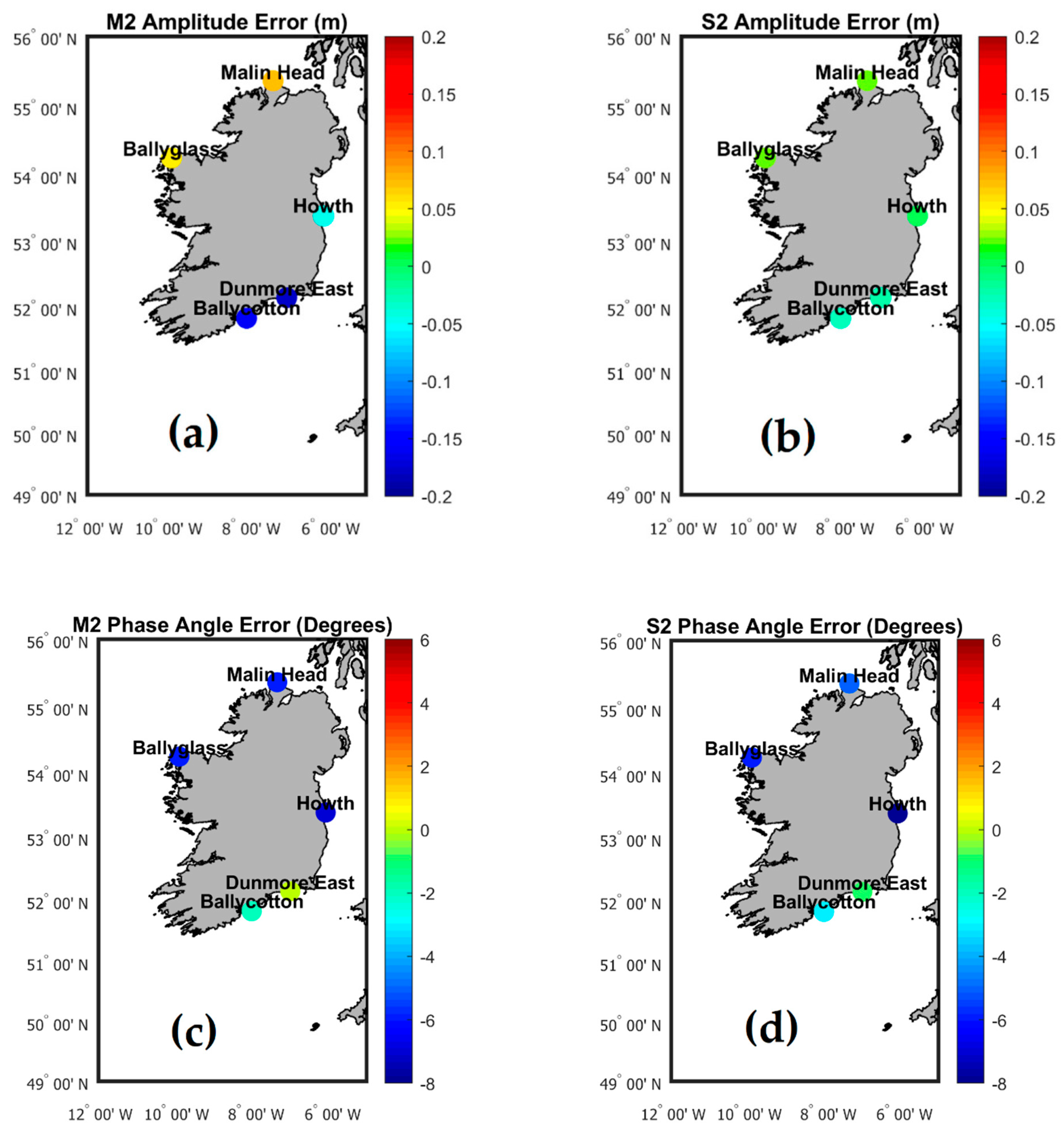
3.2. Validation of NEA_ROMS Sea Surface Height against Tide Gauge Stations

Observed time series from tide gauges around the Irish coast are compared with model sea surface heights output at the same locations as shown in Figure 5, Table 2 and Table 3. The tide gauge stations are distributed around the whole of the Republic of Ireland. Harmonic analysis was carried out on the eight locations using the T-TIDE software in MATLAB [62]. The aim of the analysis was to compare the modelled and measured values of the main tidal constituents (magnitude and phase angle). This analysis demonstrated that the tidal signal in the Sea Surface Height (SSH) data was dominated by three semi-diurnal constituents (M2, S2, N2) and three diurnal constituents (K1, O1, and Q1). Regarding our tidal analysis the authors found that M2 and S2 are responsible for most of the tide in our domain in agreement with [76,77,78,79]. The spatial variability in the mean error between model and observations for the two main constituents, M2 and S2, is shown in Figure 5a–d. The model shows good skills on the west coast of Ireland and also in the western Irish Sea. The maximum M2 magnitude error for the west Irish coast was about 0.07 m for Malin Head, Aranmore, and Galway tide gauge stations. However, the model has a higher negative error of about 5% of the total M2 amplitude in the Celtic Sea recorded in Dunmore East tide gauge station where the M2 amplitude is consistently underestimated. The S2 amplitude error shows a broadly similar pattern of M2. The maximum S2 error of about (-) 0.03 m (about 6% of the total S2 amplitude) was recorded in the Celtic Sea at the Ballycotton tide gauge station. One explanation for the poorer skill in the Celtic Sea is an excessive dissipation of tidal energy over the broad expanse of shelf south of Ireland, leading to a reduction in the amplitude of the tidal wave in agreement with [80]. The phase angle errors for both components M2 and S2 are negative at most tide gauges stations except in Dunmore East station as shown in Figure 5c,d. The highest negative phase angle error for both components was found to be (-) 7° in the Celtic Sea and also recorded at the Howth gauge station. The aggregated results for the most significant tidal constituents are presented in Table 2. The magnitude difference was very small for all tidal constituents. Ratios of the modelled to the observed amplitudes of the constituents show that the model has good skill at N2, O1, and Q1 though these constituents are much less significant to the total tide than the other three.
Accurate prediction of the surge is vital if a model is to be effective as part of a coastal flooding early warning system. The surge component was calculated following [63], for observed and modelled data at the locations of Irish tide gauges and the different statistics are presented in Table 3. Surge is caused by atmospheric pressure and wind. In order to obtain the surge signal we removed tides. The tidal signal in the Sea Surface Height (SSH) data was dominated by three semi-diurnal constituents (M2, S2, N2,) and three diurnal constituents (K1, O1, and Q1). The bias results were approximately zero for most gauge stations except in Ballyglass, Dunmore East, and Malin Head that were −0.01, 0.01, and 0.01 m respectively. The results show that the RMSE is around 0.15 m for all gauge stations. There are a number of possible contributors to this error, including the slight phase difference in the tidal signal and inaccuracies in the modelled weather fields both in space and time.

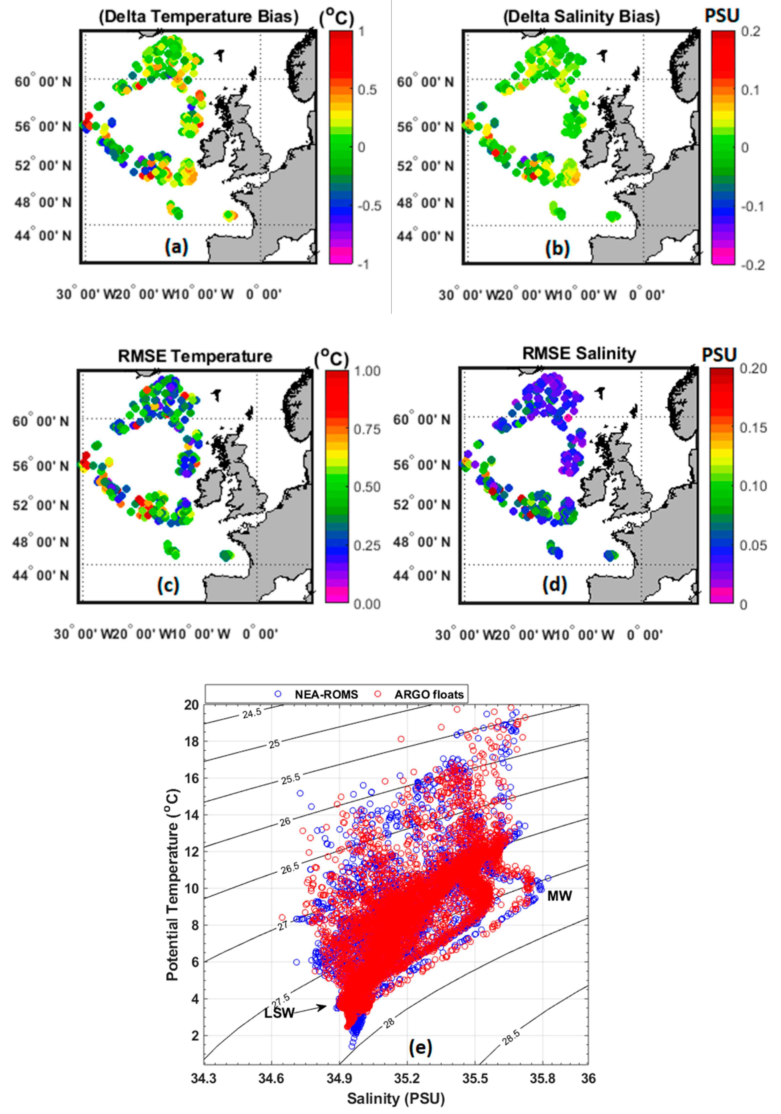
3.3. Validation of NEA_ROMS with ARGO Floats Temperature and Salinity Profiles

The locations of ARGO float profiles in the NEA_ROMS domain are shown in Figure 6a–e. The authors used 304 quality checked ARGO profiles data for the year 2019. The bias between modelled and measured ARGO float temperature and salinity profiles are presented in Figure 6a,b. The bias results reveal an agreement between NEA_ROMS and ARGO temperature and salinity profiles for most of the locations. The maximum bias between the NEA_ROMS and Argo floats temperature was 0.8 °C and located at the western open boundary (see Figure 6a). The same locations recorded maximum salinity bias of around 0.15. This may be due to the fact that some of the Argo floats are located too close to the boundary where they are influenced by boundary nudging effects. Additionally, the absence of the wave effect in our model could be an important reason for poor representation of the salinity and temperature across the water column as described in [74]. Biases were used to calculate the RMSE as shown in Figure 6c,d. The maximum RMSE between the NEA_ROMS and Argo floats temperature was 1 °C at the same locations described above. The RMSE magnitude of the temperatures is warmer in the model than measured. While the maximum RMSE for the salinity was about 0.15 and recorded again at the northwestern open boundary edge as seen in Figure 6d. This can be attributed to the reason mentioned above. The NEA model correctly reproduces salinity/temperature profiles in the inner domain and high latitude areas. Figure 6e shows the T-S diagram for both model and ARGO float profiles combined with σθ contours, while, the water masses description for the Rockall Trough area according to [24,81] is shown in Figure 7. Figure 6e suggests that ARGO and model output broadly match. The model could describe the high saline dense Mediterranean Water (MW). This water mass is located to the south of the Porcupine Bank at 1000 m depth with a maximum salinity of about 35.8, temperature range from 8 to 10 °C, and a σθ of approximately 27.6 in agreement with [82]. In addition, the deep water mass of Labrador Sea Water (LSW) is well developed by the model and ARGO floats T-S diagram. This cold deep water mass is generated over the Labrador basin and slowly makes its way east across the Atlantic Ocean [83]. This water mass is found at 2000 m depth with a salinity of about 34.8, temperature 3 °C, and σθ of approximately 27.8 in agreement with [83,84,85] and shown by Figure 6e and Figure 7. The water mass Subarctic Intermediate Water (SAIW) signal is presented by Model and ARGO floats T-S diagram. This water mass is located at the northern entrance to the Rockall Trough at 900 m depth with a maximum salinity of about 35.2 and σθ of approximately 27 as shown in Figure 6e and Figure 7, and described by [86]. There was a problem in presenting the surface water mass Eastern North Atlantic Water ENAW at the model T-S diagram. The model does not properly recreate this signal maybe because it mixed with the underneath SAIW water mass. This may be as indirect effect of model excess vertical mixing due to the use of associated parameters with KPP vertical turbulent closure scheme as described in [46,47]. This parameters were used to tune the vertical profiles of currents, temperature, and salinity [46,47]. In conclusion, the comparison with ARGO floats profiles has shown a good capability of the model to reproduce the main structures of the field in the area.

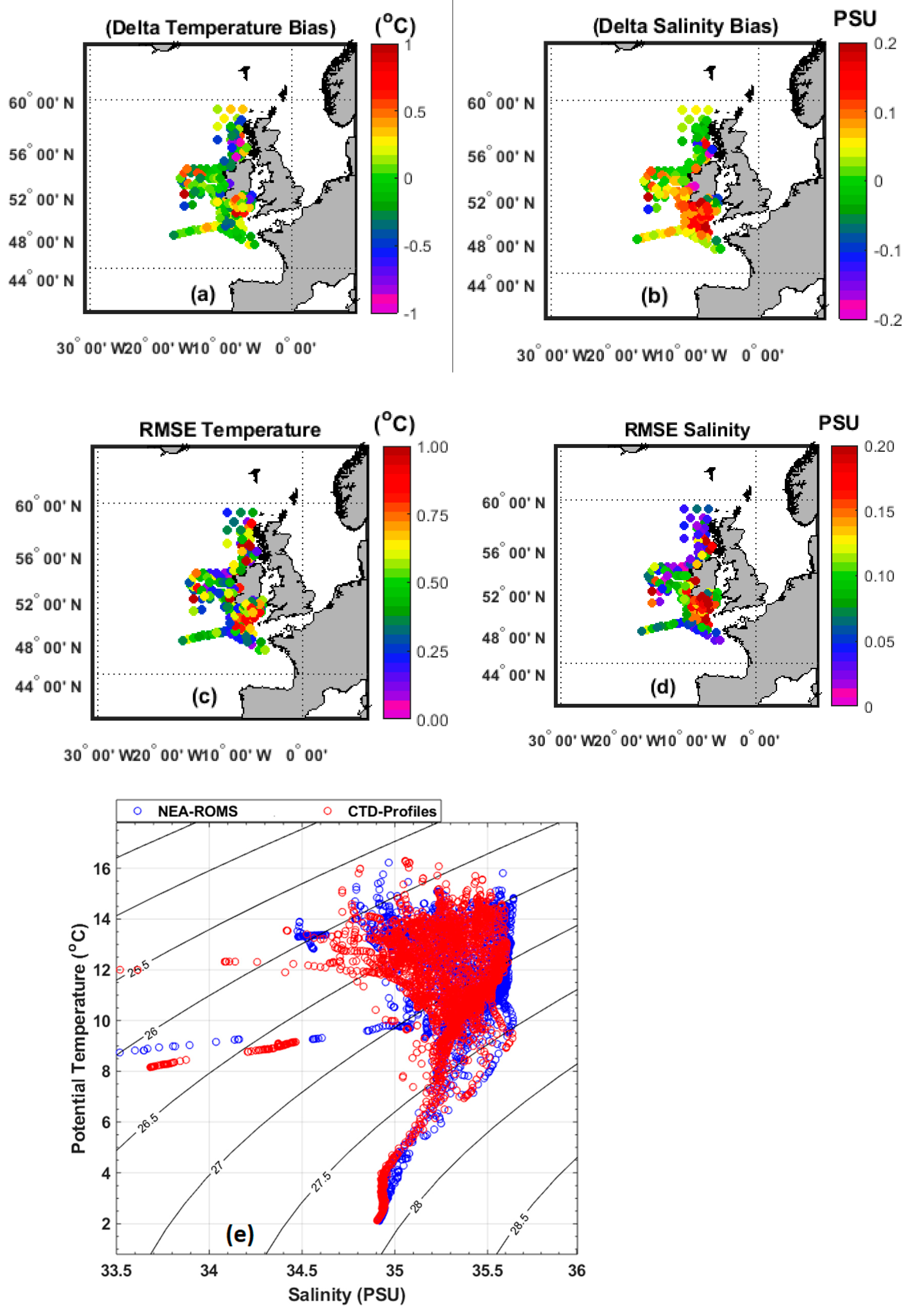
3.4. Validation of NEA_ROMS with CTDs Temperature and Salinity Profiles

To measure the model performance in shelf waters IMI used Conductivity Temperature Depth (CTD) profiles. The method used to compare the model and CTD data is the same as that used for the ARGO data. The authors analyzed 223 CTD profiles From January 2017 to December 2017, CTDs were acquired from the IMI research vessels in the shelf seas around Ireland as shown in Figure 8a–d. This data was analyzed to assess the model performance in the shallow, coastal waters around Ireland. Figure 8a,b presents the bias between modelled and measured CTD temperature and salinity profiles. The temperature bias results propose a good agreement between NEA_ROMS and CTD profiles as shown in Figure 8a. The temperature bias results are almost zero for most locations except one profile situated to the west of the Irish coast. The temperature bias in this single location was found to be 0.9 °C. The salinity bias results suggest an overestimation by the NEA_ROMS of about 0.15 for most profiles located at the southern entrance to the Irish Sea (see Figure 8b). The reason behind this could be related to the lower accuracy of the salinity field for the CMEMS model in this area. The CMEMS salinity field has improved a lot since 2017 as described in [87]. This improvement would obviously have a big impact on our model salinity field. The maximum RMSE between the model and the CTD temperature profiles was found to be 0.8 °C while it was 0.17 for salinity as described in Figure 8c,d. The distribution patterns of the RMSE values clearly show the model robustness in presenting the main water masses at the Irish shelf waters.
The T-S diagram for NEA_ROMS and 223 CTDs profiles describes the Irish coastal waters around Ireland as shown in Figure 8e. The comparison between the CTDs T-S diagram and the model T-S shows a very good agreement. We observed a significant resemblance in the T-S diagram patterns between the CTD data and the model in the whole water column. The NEA_ROMS T-S diagram represents deep water masses well, while it overestimates salinities in some surface shallow coastal waters with maximum centered salinity of about 35.5 and σθ of approximately 26.5 as shown in Figure 8b. The reason for the overestimation model salinity is probably a significant underestimation of the discharge of fresh water into the coastal waters of Ireland and west Britain. Another possibility, as previously mentioned, may be due to the use of KPP vertical turbulent closure scheme inside the ROMS model which can affect the vertical mixing as described in [46,47]. This issue is a potential source of deficiencies between model output and observations.
In conclusion, the NEA model correctly reproduces the shelf water masses around Ireland.

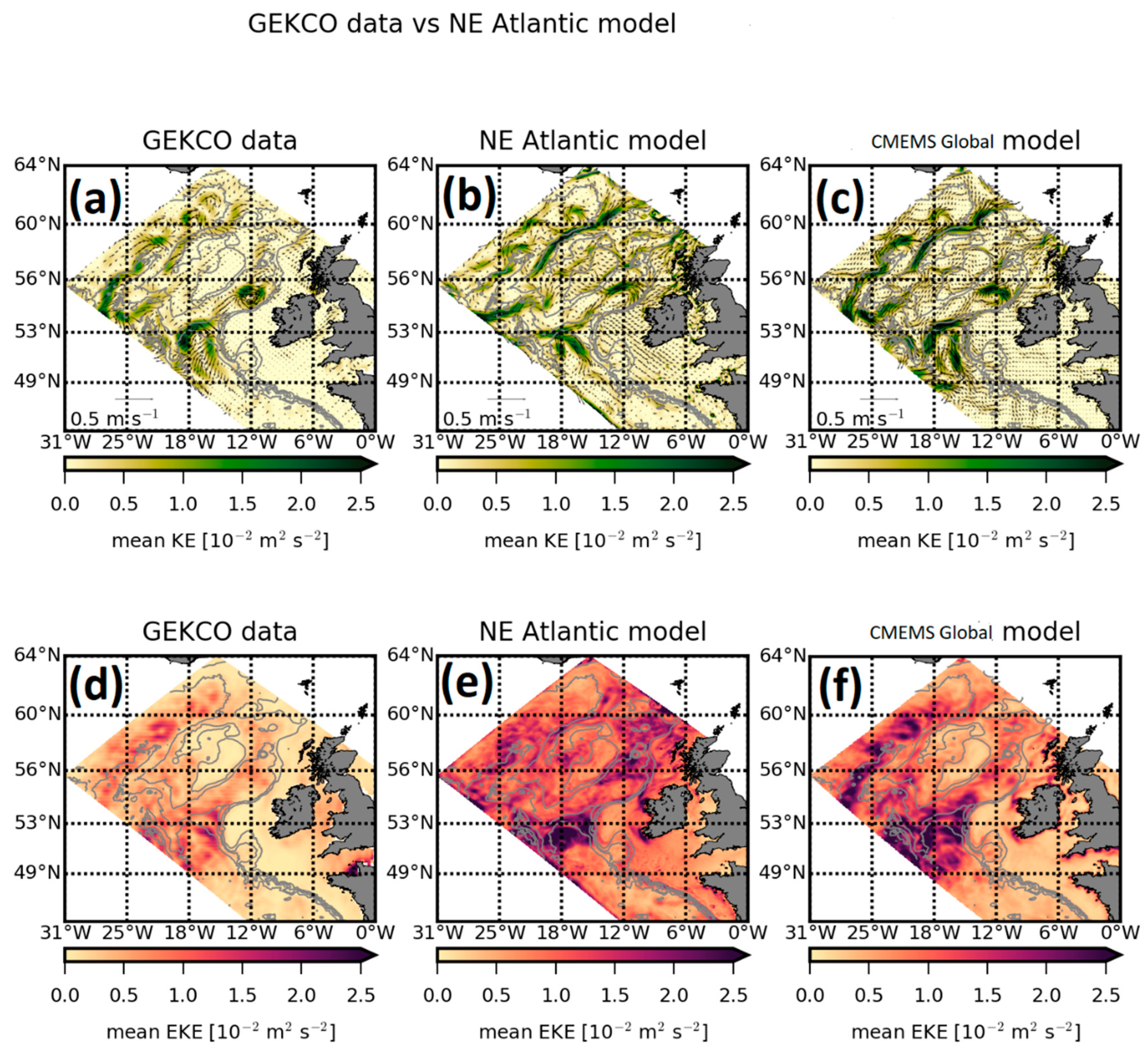
3.5. Validation of NEA_ROMS with GEKCO Surface Data

Mean Kinetic Energy (MKE) and EKE calculated from geostrophic current from altimetry GEKCO data and surface current from NEA and CMEMS global models are shown in Figure 9 which was previously described in Section 2.4. The authors combined surface current with MKE maps in Figure 9a–c to validate NEA_ROMS current pattern. The GEKCO data and both models are characterized by the North Atlantic Current and European Slope Current which transports heat and salt from the north-east Atlantic, interacts with the continental shelf slope and forms branches that flow into the North Sea in agreement with [23,35]. Both NEA_ROMS and CMEMS Global models produce similar mean circulation to the GEKCO currents. NEA_ROMS has well-resolved meanders and eddies, which are not well-resolved by CMEMS global (see Figure 9b). For example, the eddies and meanders associated with the North Atlantic Current at the middle of NEA_ROMS domain seem to be realistic as shown before by [32,35,88]. The NEA_ROMS has a higher resolution and more detailed bathymetry in this area than the CMEMS model, and this is probably the reason that it is better able to resolve the eddy field in the area. Figure 9a–c suggests that CMEMS global model generally has the largest MKE field, except for the North Ireland region. However, CMEMS global assimilates observations such as altimetric sea level, temperature and salinity profiles, and corrects toward satellite SST at the surface, as described in [87], so that MKE could be larger at times due to the correction of physics uncertainties [73,89]. Figure 9e–f represents the mean EKE fields for GEKCO data, NEA_ROMS, and CMEMS global, respectively. The basin averaged EKE for GEKCO data, NEA_ROMS, and CMEMS were 0.0063, 0.0153, and 0.0147 m2 s−2, respectively. The EKE comparison suggests the NEA_ROMS has the highest EKE field. The finer model resolution and the better river discharges of NEA_ROMS may produce this change according to [73,90]. Overall, NEA_ROMS reproduces the main regional circulation patterns, improving the dynamics forced by finer resolution and more detailed bathymetry in this area.

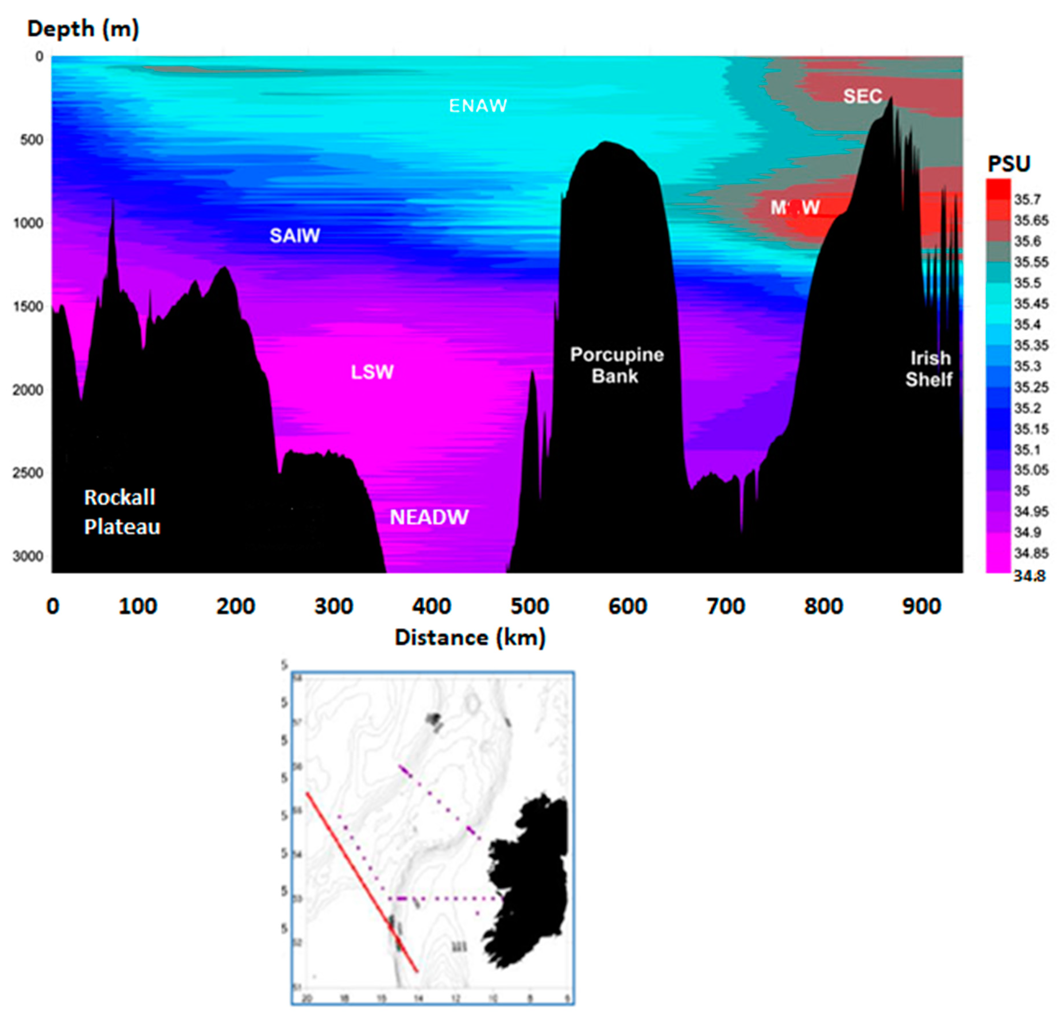
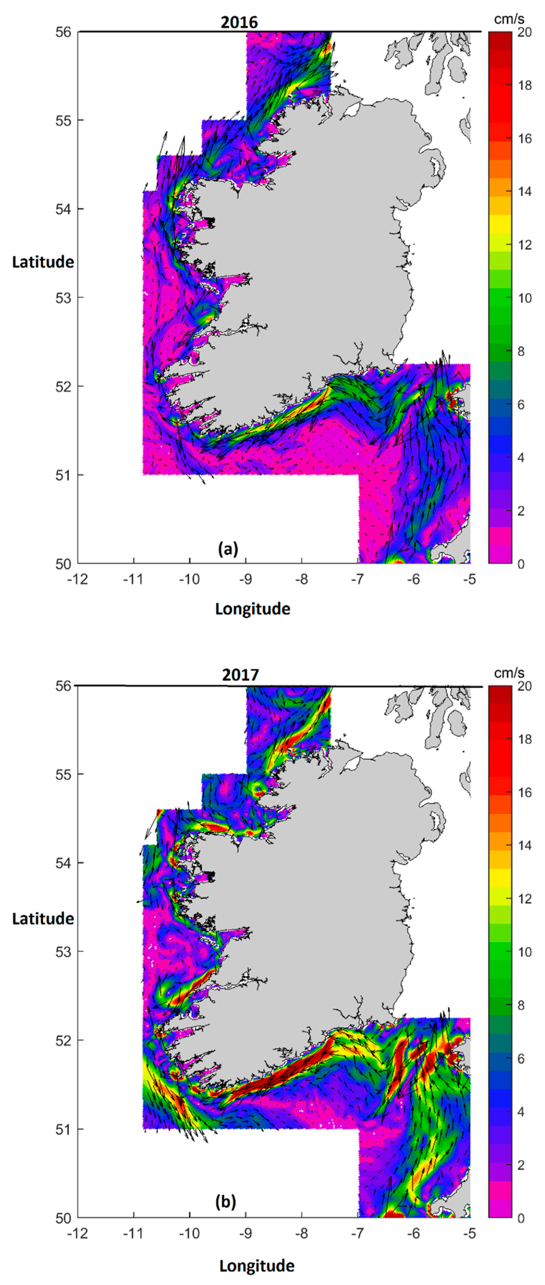
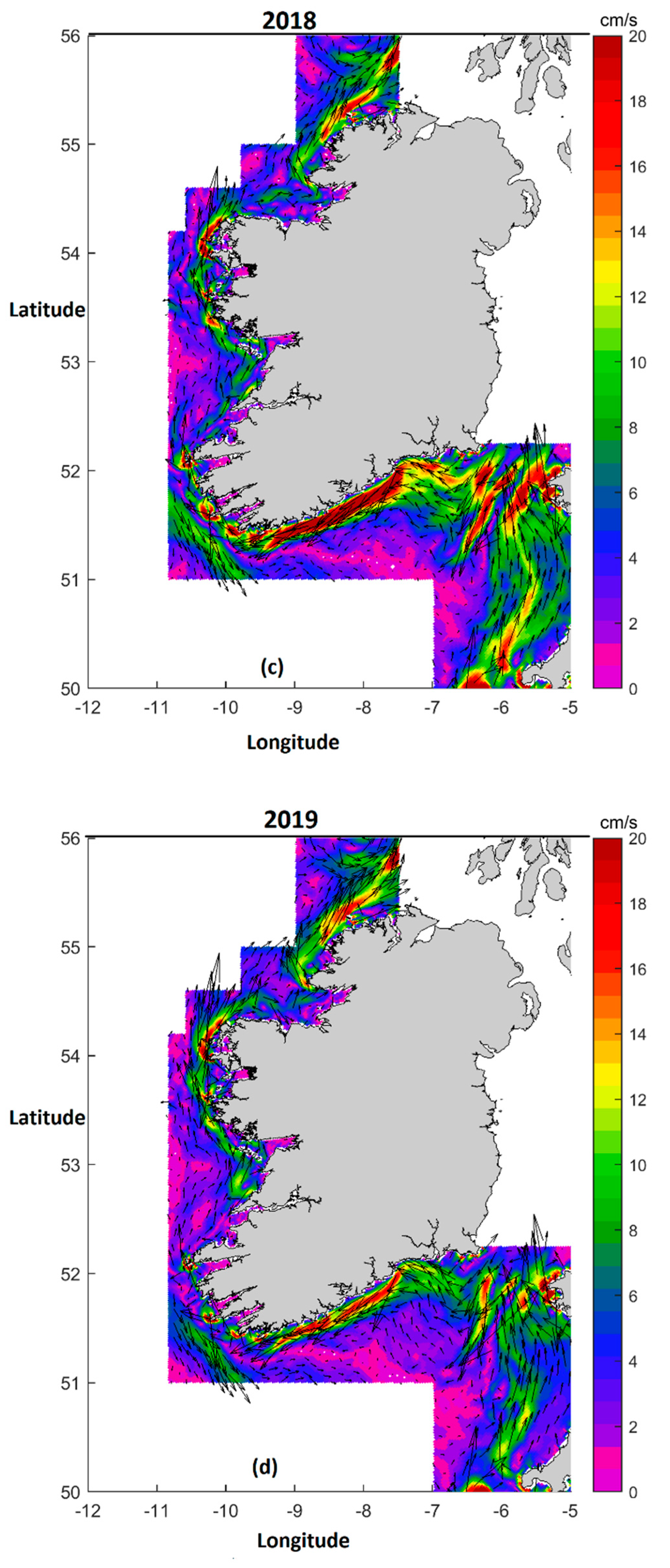
4. The Irish Coast Current (ICC)

Whilst it is fundamental that a hydrodynamic model is quantitatively validated, it is also necessary that it reproduces the important hydrographical features within its domain. To that end, an assessment is made of the model’s ability to reproduce the summer Irish Coastal Current (ICC) [10,11,91]. The ICC flows northward parallel to the western coast of Ireland [92]. The flow of ICC depends on the local wind forcing, so the Atlantic Water then either enters the Irish Sea through the North Channel or, more likely, continues flowing northward producing the ICC until the Hebrides [92]. Additionally, the ICC shows a shelf-located meandering surface current of 10–20 cm·s−1 which, has a full depth presence over the 100–120 m contours [93,94]. The authors followed the methodology of [11] to produce the annual maps of the summer ICC simply by averaging two months (July and August) of the mid-depth residual NEA_ROMS velocity field for the Celtic Sea and Irish Shelf. We used the model output hourly snapshots velocity field. To produce annual maps, we get velocities away from ICC region out of the picture.
Figure 10 displays the annual results for this analysis over the whole simulation period from 2016 until 2019. The velocity of the current is found to be in the range of 6–20 cm s−1 which is in agreement with reported values in the published literature [10,11]. The localized “hotspots” of increased velocities near headlands on the western coast are presumably induced by the tidal current while the weakening of the current north of the Shannon may be indicative of tidal mixing being more dominant than stratification [11,93]. The map patterns suggest a well-developed ICC for all years except for 2016. The highest velocity for the ICC was about 19 cm s−1 and recorded in 2017, 2018, and 2019 as shown in Figure 10b–d. There is an interesting difference in 2019 where the ICC is very strong and well defined along most of the western Irish coast (see Figure 10d). In conclusion, the results show that the NEA_ROMS has reproduced the ICC front for the whole simulation period.

5. Conclusions and Further Discussion

This paper presents an operational model for Irish waters NEA_ROMS. The model is based on ROMS and is forced by operationally available atmospheric and boundary data. The system is robust following several years in operation and model data is made freely available via THREDDS server. The authors validated and calibrated the NEA_ROMS with available observations in our domain area. The observations were the SST obtained from satellite covering the simulation period, time series of eight tide gauges around the Irish coast obtained from the Irish National Tide Gauge Network, Argo, and CTD temperature and salinity profiles.
The SST for the NEA_ROMS bias was greater than the satellite during the summer months of June and July over the whole simulation period. The highest daily bias mean was about 1.8 °C and recorded in mid-June 2018. While the lowest daily bias mean was −0.8 °C in mid-November 2019. The authors attribute this to the model error as a result of air–sea physics parametrizations as discussed by [71,72,73]. The highest correlation coefficient was found to be more than 0.97 and recorded in March and April 2018. While, the minimum correlation coefficient was 0.85 and recorded in mid-June 2018 and December 2019.
The model has a higher negative error of about 5% of the total M2 amplitude in the Celtic Sea recorded in Dunmore East tide gauge station. The S2 amplitude error showed a broadly similar pattern to M2. The maximum S2 error was about 6% of the total S2 amplitude recorded in the Celtic Sea at the Ballycotton tide gauge station. That was due to the poorer skill in the Celtic Sea due to excessive dissipation of tidal energy over the broad expanse of shelf south of Ireland, leading to a reduction in the amplitude of the tidal wave in agreement with [80].
The validation of NEA_ROMS with ARGO floats revealed the model skills in representing the main water masses in particular MW and LSW for the area located to the south of the Porcupine Bank and the entrance to the Rockall Trough. The location of some Argo floats too close to the boundary has increased the temperature and salinity RMSE because they may have been influenced by model boundary nudging effects.
The maximum RMSE between the model and the CTD temperature profiles was found to be 0.8 °C while it was 0.17 for salinity. The NEA model correctly reproduces the shelf water masses around Ireland.
The use of KPP vertical turbulent closure scheme in the ROMS model can affect the vertical mixing of the salinity and temperature profiles as described in [46,47]. This issue was a potential source of deficiencies between model predictions and observations.
The meanders and eddies at the model domain were well resolved by NEA_ROMS which were not well resolved by CMEMS global. The NEA_ROMS has a higher resolution and more detailed bathymetry in this area, which may be the reasons why the model resolved these meanders and eddies well.
In 2019 the ICC was very strong and well defined along most of the western Irish coast. In conclusion, the results showed that the NEA_ROMS well reproduced the ICC front for the whole simulation period.
Future work requires the use of high frequency near real time river discharges. The inclusion of data assimilation in the NEA_ROMS operational system is considered to be the next logical step in its ongoing development. Recent applications also include the modelling studies of the biogeochemical cycling. Additionally, indices supporting the implementation of the Marine Strategy Framework Directive (MSFD) are usually obtained from in-situ data. This is a major difficulty in oceanic areas where data are scarce. Validated numerical models can fill this gap. Tools will be developed to obtain indices of interest directly from model results, e.g., areas of upwelling, fronts, eddy index, primary production, trophic status, or even conditions for propagation of noise.

Author Contributions

Conceptualization, H.N., K.L., G.N., T.D. and M.C.; methodology, H.N. and K.L.; The developer of the first version of the North East Atlantic model, M.C.; validation, H.N., K.L., G.N. and T.D.; formal analysis, H.N., K.L., G.N. and T.D., investigation, H.N., K.L., G.N. and T.D.; resources, H.N., K.L., G.N., T.D. and M.C.; data curation, H.N., K.L., G.N., T.D. and M.C.; writing—original draft preparation, H.N. K.L., G.N., T.D. and M.C.; writing—review and editing, K.L., G.N., T.D. and M.C.; visualization, H.N., K.L., G.N., and T.D.; supervision, G.N. and T.D.; project administration, G.N. and T.D.; funding acquisition, INTERREG Atlantic Area Cross-border Cooperation Programme project “Innovation in the Framework of the Atlantic Deep Ocean” (iFADO, under contract EAPA 165/2016. All authors have read and agreed to the published version of the manuscript.

Funding

The validation of the model was funded by the INTERREG Atlantic Area Cross-border Cooperation Programme project “Innovation in the Framework of the Atlantic Deep Ocean” (iFADO, under contract EAPA 165/2016).

Acknowledgments

The authors are grateful to INTERREG Atlantic Area Cross-border Cooperation Programme project “Innovation in the Framework of the Atlantic Deep Ocean” (iFADO, under contract EAPA 165/2016) for supporting this study. We wish to thank Maximo Garcia-Jove Navarro for processing GEKCO and CMEMS data and developing Figure 9. Finally, we would like to thank Achref Othmani for preparing Table 1 the mean annual climatological river discharge values that were included in the NEA_ROMS. Special thanks to the two anonymous reviewers for helpful comments on the manuscript.

Conflicts of Interest

The authors declare no conflict of interest.

References

  1. McCartney, M.S.; Mauritzen, C.M. On the origin of the warm inflow to the Nordic Seas. Prog. Oceanogr. 2001, 51, 125–214. [Google Scholar] [CrossRef]
  2. Holliday, N.P.; Pollard, R.T.; Read, J.F.; Leach, H. Water mass properties and fluxes in the Rockall Trough, 1975–1998. Deep Sea Res. 2000, 47, 1303–1332. [Google Scholar] [CrossRef]
  3. Holliday, N.P.; Bacon, S.; Cunningham, S.A.; Gary, S.F.; Karstensen, J.; King, B.A.; Li, F.; Mcdonagh, E.L. Subpolar North Atlantic Overturning and Gyre-Scale Circulation in the summers of 2014 and 2016. J. Geophys. Res. Ocean. 2018, 123, 4538–4559. [Google Scholar] [CrossRef]
  4. Pingree, R.D.; Le Cann, B. 1989. Celtic and Armorican slope and shelf residual currents. Prog. Oceanogr. 1989, 23, 303–338. [Google Scholar] [CrossRef]
  5. Turrell, W.R.; Jorge da Silva, A.; Mohn, C.; Griffiths, C.; Lavin, A.; Svendsen, E.; White, M. A Quasi-Synoptic Survey of the European Continental Shelf Edge during the SEFOS Project; ICES CM 1995, 1995/C:10; Hydrography Committee: Copenhagen, Denmark, 1995. [Google Scholar]
  6. Pingree, R.D.; Sinha, B.; New, A.L.; Waddington, I.; Head, R.N.; Nechvolodov, L.V. Will deep subtropical ring ‘Storm Physalia’ cross the Mid Atlantic Ridge and reach America? Mar. Biol. Assoc. UK 1996, 76, 553–567. [Google Scholar] [CrossRef]
  7. Huthnance, J.M.; Holt, J.T.; Wakelin, S.L. Deep ocean exchange with west-European shelf seas. Ocean Sci. 2009, 5, 621–634. [Google Scholar] [CrossRef] [Green Version]
  8. Huang, W.G.; Cracknell, A.P.; Vaughan, R.A.; Davies, P.A. A satellite and field view of the Irish Shelf Front. Cont. Shelf Res. 1991, 11, 543–562. [Google Scholar] [CrossRef]
  9. McCarthy, T.K.; Frankiewicz, P.; Cullen, P.; Blaszkowski, M.; O’Connor, W.; Doherty, D. Long term effects of hydropower installations and associated river regulation on River Shannon eel populations: Mitigation and management. Hydrobiologia 2008, 609, 109–124. [Google Scholar] [CrossRef]
  10. Brown, J.; Carillo, L.; Fernand, L.; Horsburgh, K.J.; Hill, A.E.; Young, E.F. Observations of the physical structure and seasonal jet-like circulation of the Celtic Sea and St. George’s Channel of the Irish Sea. Cont. Shelf Res. 2003, 23, 533–561. [Google Scholar] [CrossRef]
  11. Fernand, L.; Nolan, G.D.; Raine, R.; Chambers, C.E.; Dye, S.R.; White, M.; Brown, J. The Irish coastal current: A seasonal jet-like circulation. Cont. Shelf Res. 2006, 26, 1775–1793. [Google Scholar] [CrossRef]
  12. Hill, A.E.; Simpson, J.H. Low frequency variability of the Scottish Coastal Current induced by alongshore pressure gradients. Estuar. Coast. Shelf Sci. 1988, 27, 163–180. [Google Scholar] [CrossRef]
  13. Pinardi, N.; Allen, I.; Demirov, E.; De Mey, P.; Korres, G.; Lascratos, A.; Le Traon, P.Y.; Maillard, C.; Manzella, G.; Tziavos, C. Mediterranean Forecasting System: First Phase of Implementation (1998–2001). J. Ann. Geophys. 2003, 21, 1–21. [Google Scholar] [CrossRef] [Green Version]
  14. Holt, M.; Li, Z.; Osborne, J. Real time forecast modeling for the NW European Shelf Seas. In Building the European Capacity in Operational Oceanography; Elsevier Oceanography Series; Dahlin, H., Flemming, N.C., Nittis, K., Petersson, S.E., Eds.; Elsevier Science: Amsterdam, The Netherlands, 2003; Volume 69, pp. 484–489. [Google Scholar]
  15. Cure, M.; Lyons, K.; Nolan, G. Operational Forecasting in the IBIROOS Region. In Proceedings of the Adjoint Modeling and Applications, La Jolla, CA, USA, 24–26 October 2005. [Google Scholar]
  16. Elliott, A.; Hartnett, M.; O’Riain, G.; Dollard, B. The PRISM Project: Predictive Irish Sea Models; Final Report; Catchment to Coast Research Centre University of Wales Aberystwyth and Bangor Ceredigion: Cardiff, UK, 2007. [Google Scholar]
  17. Siddorn, J.R.; Allen, J.I.; Blackford, J.C.; Gilbert, F.J.; Holt, J.T.; Holt, M.W.; Osborne, J.P.; Proctor, R.; Mills, D.K. Modelling the hydrodynamics and ecosystem of the North-West European continental shelf for operational oceanography. Mar. Syst. 2007, 65, 417–429. [Google Scholar] [CrossRef]
  18. Kordzadze, A.A.; Demetrashvili, D.I. Operational forecast of hydrophysical fields in the Georgian Black Sea coastal zone within the ECOOP. Ocean Sci. 2011, 7, 793–803. [Google Scholar] [CrossRef] [Green Version]
  19. Korotaev, G.K.; Oguz, T.; Dorofeyev, V.L.; Demyshev, S.G.; Kubryakov, A.I.; Ratner, Y.B. Development of Black Sea nowcasting and forecasting system. Ocean Sci. 2011, 7, 629–649. [Google Scholar] [CrossRef] [Green Version]
  20. Stanev, E.V.; Schulz-Stellenfleth, J.; Staneva, J.; Grayek, S.; Seemann, J.; Petersen, W. Coastal observing and forecasting system for the German Bight estimates of hydrophysical states. Ocean Sci. 2011, 7, 569–583. [Google Scholar] [CrossRef] [Green Version]
  21. Zhuang, S.Y.; Fu, W.W.; She, J. A pre-operational three dimensional variational data assimilation system in the North/Baltic Sea. Ocean Sci. 2011, 7, 771–781. [Google Scholar] [CrossRef] [Green Version]
  22. Mateus, M.; Riflet, G.; Chambel, P.; Fernandes, L.; Fernandes, R.; Juliano, M.; Campuzano, F.; de Pablo, H.; Neves, R. An operational model for the West Iberian coast: Products and services. Ocean Sci. 2012, 8, 713–732. [Google Scholar] [CrossRef] [Green Version]
  23. Siddorn, J.R.; Furner, R. An analytical stretching function that combines the best attributes of geopotential and terrain-following vertical coordinates. Ocean Model. 2013, 66, 1–13. [Google Scholar] [CrossRef]
  24. Dabrowski, T.; Lyons, K.; Berry, A.; Cusack, C.; Nolan, G. An operational biogeochemical model of the North-East Atlantic: Model description and skill assessment. J. Mar. Syst. 2014, 129, 350–367. [Google Scholar] [CrossRef]
  25. Danabasoglu, G.; Yeager, S.G.; Bailey, D.; Behrens, E.; Bentsen, M.; Bi, D.; Biastoch, A.; Böning, C.; Bozec, A.; Canuto, V.M.; et al. North Atlantic simulations in Coordinated Ocean-ice Reference Experiments phase II (CORE-II). Part I: Mean states. Ocean Model. 2014, 73, 76–107. [Google Scholar] [CrossRef] [Green Version]
  26. Storkey, D.; Blaker, A.T.; Mathiot, P.; Megann, A.; Aksenov, Y.; Blockley, E.W.; Calvert, D.; Graham, T.; Hewitt, H.T.; Hyder, P.; et al. UK Global Ocean GO6 and GO7: A traceable hierarchy of model resolutions. Geosci. Model Dev. 2018, 11, 3187–3213. [Google Scholar] [CrossRef] [Green Version]
  27. Gutknecht, E.; Reffray, G.; Mignot, A.; Dabrowski, T.; Sotillo, M.G. Modelling the marine ecosystem of Iberia–Biscay–Ireland (IBI) European waters for CMEMS operational applications. Ocean Sci. 2019, 15, 1489–1516. [Google Scholar] [CrossRef] [Green Version]
  28. Fennel, K.; Wilkin, J.; Levin, L.; Moisan, J.; O’Reilly, J.; Haidvogel, D. Nitrogen cycling in the Middle Atlantic Bight: Results from a three-dimensional model and implications for the North Atlantic nitrogen budget. Glob. Biogeochem. Cycles 2006, 20, GB3007. [Google Scholar] [CrossRef] [Green Version]
  29. O’Dea, E.J.; Arnold, A.K.; Edwards, K.P.; Furner, R.; Hyder, P.; Martin, M.J.; Siddorn, J.R.; Storkey, D.; While, J.; Holt, J.T.; et al. An operational ocean forecast system incorporating NEMO and SST data assimilation for the tidally driven European North-West shelf. Oper. Oceanogr. 2012, 5, 3–17. [Google Scholar] [CrossRef] [Green Version]
  30. Sotillo, M.G.; Cailleau, S.; Lorente, P.; Levier, B.; Aznar, R.; Reffray, G.; Amo-Baladrón, A.; Chanut, J.; Benkiran, M.; Alvarez-Fanjul, E. The My Ocean IBI Ocean Forecast and Reanalysis Systems: Operational products and roadmap to the future Copernicus Service. Oper. Oceanogr. 2015, 8, 63–79. [Google Scholar] [CrossRef]
  31. Guihou, K.; Polton, J.; Wakelin, S.; O’Dea, E.; Holt, J. Kilometric Scale modeling of the North West European Shelf Seas: Exploring the spatial and temporal variability of internal tides. Geophys. Res. 2017, 123, 688–707. [Google Scholar] [CrossRef] [Green Version]
  32. Graham, J.A.; O’Dea, E.; Holt, J.; Polton, J.; Hewitt, H.T.; Furner, R.; Guihou, K.; Brereton, A.; Arnold, A.; Wakelin, S.; et al. AMM15: A new high-resolution NEMO configuration for operational simulation of the European north-west shelf. Geosci. Model Dev. 2018, 11, 681–696. [Google Scholar] [CrossRef] [Green Version]
  33. King, R.; While, J.; Martin, M.J.; Lea, D.J.; Lemieux-Dudon, B.; Waters, J.; O’Dea, E. Improving the initialisation of the Met Office operational shelf-seas model. Ocean Model. 2018, 130, 1–14. [Google Scholar] [CrossRef]
  34. Tinker, J.; Krijnen, J.; Wood, R.; Barciela, R.; Dye, S.R. What are the prospects for seasonal prediction of the marine environment of the North-west European Shelf? Ocean Sci. 2018, 14, 887–909. [Google Scholar] [CrossRef]
  35. Tonani, M.; Sykes, P.; King, R.R.; McConnell, N.; Péquignet, A.C.; O’Dea, E.; Graham, J.A.; Polton, J.; Siddorn, J. The impact of a new high-resolution ocean model on the Met Office North-West European Shelf forecasting system. Ocean Sci. 2019, 15, 1133–1158. [Google Scholar] [CrossRef] [Green Version]
  36. Ghantous, M.; Ayoub, N.; De Mey-Frémaux, P.; Vervatis, V.; Marsaleix, P. Ensemble Downscaling of a Regional Ocean Model. Ocean Model. 2020, 145, 101511. [Google Scholar] [CrossRef]
  37. Haidvogel, D.B.; Arango, H.; Budgell, W.P.; Cornuelle, B.D.; Curchitser, E.; Di Lorenzo, E.; Fennel, K.; Geyer, W.R.; Hermann, A.J.; Lanerolle, L.; et al. Ocean forecasting in terrain-following coordinates: Formulation and skill assessment of the Regional Ocean Modeling System. Comput. Phys. 2008, 227, 3595–3624. [Google Scholar] [CrossRef]
  38. Chiggiato, J.; Oddo, P. Operational ocean models in the Adriatic Sea: A skill assessment. Ocean Sci. 2008, 4, 61–71. [Google Scholar] [CrossRef] [Green Version]
  39. Chao, Y.; Li, Z.; Farrara, J.; McWilliams, J.C.; Bellingham, J.; Capet, X.; Chavez, F.; Choi, J.K.; Davis, R.; Doyle, J.; et al. Development, implementation and evaluation of a data-assimilative ocean forecasting system off the central California coast. Deep Sea Res. II 2009, 56, 100–126. [Google Scholar] [CrossRef]
  40. Wilkin, J.; Zhang, W.G.; Cahill, B.; Chant, R.C. Integrating coastal models and observations for studies of ocean dynamics, observing systems and forecasting. In Operational Oceanography in the 21st Century; Schiller, A., Brassington, G., Eds.; Springer: Dordrecht, The Netherlands, 2011; pp. 487–512. [Google Scholar] [CrossRef]
  41. Shchepetkin, A.F.; McWilliams, J.C. The Regional Ocean Modeling System: A split-explicit, free-surface, topography following coordinates ocean model. Ocean Model. 2005, 9, 347–404. [Google Scholar] [CrossRef]
  42. Large, W.G.; McWilliams, J.C.; Doney, S.C. Oceanic vertical mixing: A review and a model with a nonlocal boundary layer parameterization. Rev. Geophys. 1994, 32, 363–403. [Google Scholar] [CrossRef] [Green Version]
  43. Shchepetkin, A.F.; McWilliams, J.C. A method for Computing Horizontal Pressure-Gradient Force in an Oceanic Model with a Non- Aligned Vertical Coordinate. Geophys. Res. 2003, 108, 3090. [Google Scholar] [CrossRef]
  44. Keen, T.R.; Glenn, S.M. Factors influencing hindcast skill for modelling shallow water currents during Hurricane Andrew. J. Atmos. Ocean. Technol. 1998, 15, 221–236. [Google Scholar] [CrossRef]
  45. Keen, T.R.; Glenn, S.M. Shallow water currents during Hurricane Andrew. J. Geophys. Res. 1999, 104, 23443–23458. [Google Scholar] [CrossRef]
  46. Allahdadi, M.N.; Li, C. Numerical Simulation of Louisiana Shelf Circulation under Hurricane Katrina. J. Coast. Res. 2017, 34, 67–80. [Google Scholar] [CrossRef]
  47. Allahdadi, M.N.; Li, C. Effect of Stratification on Current Hydrodynamics over the Louisiana shelf during Hurricane Katrina. Water Sci. Eng. 2017, 10, 154–165. [Google Scholar] [CrossRef]
  48. Margolin, L.; Smolarkiewicz, P.K. Antidiffusive velocities for multipass donor cell advection. Siam J. Sci. Comput. 1988, 20, 907–929. [Google Scholar] [CrossRef]
  49. Madec, G.; the NEMO team. NEMO Ocean Engine, Note du Pôle de Modélisation 27; Institut Pierre-Simon Laplace (IPSL): Paris, France, 2008; ISSN 1288–1619. [Google Scholar]
  50. Brown, J.; Joyce, A.E.; Aldridge, J.N.; Young, E.F.; Fernand, L.; Gurbutt, P.A. Further Identification and Acquisition of Bathymetric Data for Irish Sea Modelling; DETR research contract CW075; 1999. Available online: https://www.bodc.ac.uk/resources/products/data/external_products/celtic_seas/documents/bathy_doc.pdf (accessed on 28 August 2020).
  51. Haney, R.L. On the pressure gradient force over steep bathymetry in sigma coordinates ocean models. Phys. Oceanogr. 1991, 21, 610–619. [Google Scholar] [CrossRef] [Green Version]
  52. Shapiro, R. Linear filtering. Math. Comput. 1975, 29, 1094–1097. [Google Scholar] [CrossRef]
  53. Flather, R.A. A tidal model of the northwest European continental shelf. Mem. Soc. R. Sci. Liege 1976, 6, 141–164. [Google Scholar]
  54. Shchepetkin, A.; McWilliams, J. Quasi-monotone advection schemes based on explicit locally adaptive dissipation. Mon. Weather Rev. 1998, 126, 1541–1580. [Google Scholar] [CrossRef]
  55. Marchesiello, P.; McWilliams, J.C.; Shchepetkin, A. Open boundary conditions for long term integration of regional oceanic models. Ocean Model. 2001, 3, 1–20. [Google Scholar] [CrossRef]
  56. Egbert, G.D.; Erofeeva, S.Y. Efficient inverse modeling of barotropic ocean tides. Atmos. Ocean. Technol. 2002, 19, 183–204. [Google Scholar] [CrossRef] [Green Version]
  57. Chapman, D.C. Numerical treatment of cross-shelf open boundaries in a barotropic coastal ocean model. Phys. Oceanogr. 1985, 15, 1060–1075. [Google Scholar] [CrossRef] [Green Version]
  58. Zavatarelli, M.; Pinardi, N.; Kourafalou, V.H.; Maggiore, A. Diagnostic and prognostic model studies of the Adriatic Sea circulation. Seasonal variability. Geophys. Res. 2002, 107, 3004. [Google Scholar] [CrossRef] [Green Version]
  59. Nagy, H.; Di-Lorenzo, E.; El-Gindy, E. The Impact of Climate Change on Circulation Patterns in the Eastern Mediterranean Sea Upper Layer Using Med-ROMS Model. Prog. Oceanogr. 2019, 175, 244. [Google Scholar] [CrossRef]
  60. Hellerman, S.; Rosenstein, M. Normal monthly wind stress over the world ocean with error estimates. Phys. Oceanogr. 1983, 13, 1093–1104. [Google Scholar] [CrossRef] [Green Version]
  61. Beron-Vera, F.J.; Ochoa, J.; Ripa, P. A note on the boundary conditions for salt and freshwater balances. Ocean Model. 1999, 1, 111–118. [Google Scholar] [CrossRef]
  62. Pawlowicz, R.; Beardsley, B.; Lentz, S. Classical tidal harmonic analysis including error estimates in MATLAB using T_TIDE. Comput. Geosci. 2002, 28, 929–937. [Google Scholar] [CrossRef]
  63. Flather, R.A.; Williams, J.A. Climate change effects on the storm surge: Methodologies and results. In Climate Scenarios for Water-Related and Coastal Impact; ECLAT-2 Workshop Report; Beersma, J., Agnew, M., Viner, D., Hulme, M., Eds.; CRU: Norwich, UK, 2000; pp. 66–78. [Google Scholar]
  64. Argo. Argo float data and metadata from Global Data Assembly Centre (Argo GDAC). SEANOE 2020. [Google Scholar] [CrossRef]
  65. Roemmich, D.; Johnson, G.C.; Riser, S.; Davis, R.; Gilson, J.; Owens, W.B.; Garzoli, S.L.; Schmid, C.; Ignaszewski, M. The Argo program observing the global ocean with profiling floats. Oceanography 2009, 22, 34–43. [Google Scholar] [CrossRef] [Green Version]
  66. Lumpkin, R.; Centurioni, L.; Perez, R. Fulfilling observing system implementation requirements with the global drifter array. Atmos. Ocean. Technol. 2016, 33, 685–695. [Google Scholar] [CrossRef]
  67. Gasparin, F.; Guinehut, S.; Mao, C.; Mirouze, I.; Rémy, E.; King, R.R.; Hamon, M.; Reid, R.; Storto, A.; Le Traon, P.Y.; et al. Requirements for an Integrated in situ Atlantic Ocean Observing System From Coordinated Observing System Simulation Experiments. Front. Mar. Sci. 2019, 6, 83. [Google Scholar] [CrossRef] [Green Version]
  68. Sudre, J.; Maes, C.; Garçon, V. On the global estimates of geostrophic and Ekman surface currents. Limnol. Oceanogr. Fluids Environ. 2013, 3, 21–39. [Google Scholar] [CrossRef] [Green Version]
  69. Ubelmann, C.; Klein, P.; Fu, L.L. Dynamic interpolation of sea surface height and potential applications for future high-resolution altimetry mapping. J. Atmos. Ocean. Technol. 2015, 32, 177–184. [Google Scholar] [CrossRef] [Green Version]
  70. Penduff, T.; Barnier, B.; Dewar, W.K.; O’Brien, J.J. Dynamical response of the oceanic eddy field to the North Atlantic Oscillation: A model-data comparison. J. Phys. Oceanogr. 2004, 34, 2615–2629. [Google Scholar] [CrossRef]
  71. Tonani, M.; Pinardi, N.; Fratianni, C.; Pistoia, J.; Dobricic, S.; Pensieri, S.; Alfonso, M.; Nittis, K. Mediterranean Forecasting System: Forecast andanalysis assessment through skill score. Ocean Sci. 2009, 5, 649–660. [Google Scholar] [CrossRef] [Green Version]
  72. Pettenuzzo, D.; Large, W.G.; Pinardi, N. On the corrections of ERA-40 surface flux products consistent with the Mediterranean heat and water budgets and the connection between basins surface total heat flux and NAO. Geophys. Res. 2010, 115, C06022. [Google Scholar] [CrossRef]
  73. Nagy, H.; Elgindy, A.; Pinardi, N.; Zavatarelli, M.; Oddo, P. A nested pre-operational model for the Egyptian shelf zone: Model configuration and validation/calibration. Dyn. Atmos. Ocean. 2017, 80, 75–96. [Google Scholar] [CrossRef]
  74. Allahdad, M.A.; He, R.; Neary, V.S. Predicting ocean waves along the US east coast during energetic winter storms: Sensitivity to whitecapping parameterizations. Ocean Sci. 2019, 15, 691–715. [Google Scholar] [CrossRef] [Green Version]
  75. Aijaz, S.; Ghantous, M.; Babanin, A.V.; Ginis, I.; Thomas, B.; Wake, G. Nonbreaking wave-induced mixing in upper ocean during tropical cyclones using coupled hurricane-ocean-wave modeling. J. Geophys. Res. Ocean. 2017, 122, 3939–3963. [Google Scholar] [CrossRef] [Green Version]
  76. Mungall, J.C.H.; Matthews, J.B. The M2 tide of the Irish Sea: Hourly configurations of the sea surface and of the depth-mean currents. Estuar. Coast. Mar. Sci. 1978, 6, 55–74. [Google Scholar] [CrossRef]
  77. Robinson, I.S. The tidal dynamics of the Irish and Celtic Seas. Geophys. J. Int. 1979, 56, 159–197. [Google Scholar] [CrossRef]
  78. O’Rourke, F.; Boyle, F.; Reynolds, A. Tidal energy update. Appl. Energy 2009, 87, 398–409. [Google Scholar] [CrossRef]
  79. O’Rourke, F.; Boyle, F.; Reynolds, A. Tidal current energy resource assessment in Ireland: Current status and future update. Renew. Sustain. Energy Rev. 2010, 14, 3206–3212. [Google Scholar] [CrossRef] [Green Version]
  80. Pugh, D.T. Tidal amphidrome movement and energy dissipation in the Irish Sea. Geophys. J. Int. 1981, 67, 515–527. [Google Scholar] [CrossRef]
  81. McGrath, T.; Nolan, G.; McGovern, E. Chemical characteristics of water masses in the Rockall Trough. Deep Sea Res. I Oceanogr. Res. Pap. 2011, 61, 57–73. [Google Scholar] [CrossRef]
  82. Lozier, M.S.; Stewart, N.M. On the temporally varying northward penetration of Mediterranean Overflow Water and eastward penetration of Labrador Sea Water. J. Phys. Oceanogr. 2008, 38, 2097–2103. [Google Scholar] [CrossRef] [Green Version]
  83. McCartney, M.S.; Talley, L.D. The subpolar mode water of the North Atlantic Ocean. J. Phys. Oceanogr. 1982, 12, 1169–1188. [Google Scholar] [CrossRef] [Green Version]
  84. Pickart, R.S.; Spall, M.A. Impact of Labrador Sea convection on the North Atlantic meridional overturning circulation. J. Phys. Oceanogr. 2007, 37, 2207–2227. [Google Scholar] [CrossRef] [Green Version]
  85. LeBel, D.A.; Smethie, W.M.; Rhein, M.; Kieke, D.; Fine, R.A.; Bullister, J.L.; Min, D.H.; Roether, W.; Weiss, R.F.; Andrié, C.; et al. The formation rate of North Atlantic Deep Water and eighteen degree water calculate from CFC-11 inventories observed during WOCE. Deep Sea Res. I 2008, 55, 891–910. [Google Scholar] [CrossRef]
  86. Xu, X.; Rhines, P.B.; Chassignet, E.P. On mapping the diapycnal water mass transformation of the upper North Atlantic Ocean. J. Phys. Oceanogr. 2018, 48, 2233–2258. [Google Scholar] [CrossRef]
  87. Lellouche, J.M.; Greiner, E.; Le Galloudec, O.; Garric, G.; Regnier, C.; Drevillon, M.; Benkiran, M.; Testut, C.E.; Bourdalle-Badie, R.; Gasparin, F.; et al. Recent updates to the Copernicus Marine Service global ocean monitoring and forecasting real-time 1/12° high-resolution system. Ocean Sci. 2018, 14, 1093–1126. [Google Scholar] [CrossRef] [Green Version]
  88. Graham, J.; Rosser, J.P.; O’dea, E.; Hewitt, H.T. Resolving the Shelf Break Exchange around the European Northwest Shelf. Geophys. Res. Lett. 2018, 45, 12–386. [Google Scholar] [CrossRef] [Green Version]
  89. Dobricic, S.; Pinardi, N.; Adani, M.; Tonani, M.; Fratianni, C.; Bonazzi, A.; Fernandez, V. Daily oceanographic analyses by Mediterranean Forecasting System at the basin scale. Ocean Sci. 2007, 3, 149–157. [Google Scholar] [CrossRef] [Green Version]
  90. Tonani, M.; Pinardi, N.; Dobricic, S.; Pujol, I.; Fratianni, C. A high resolution free surface model on the Mediterranean sea. J. Ocean Sci. 2008, 4, 1–14. [Google Scholar] [CrossRef] [Green Version]
  91. Nolan, G.D.; Lyons, K. Ocean climate variability on the western Irish Shelf, an emerging time series. In Proceedings of the ICES Annual Science Conference, Gothenburg, Sweden, 9–12 September 2006; p. 28. [Google Scholar]
  92. Xing, J.; Davies, A.M. The influence of shelf edge flows and wind upon the circulation on the Malin Shelf and in the Irish Sea. Cont. Shelf Res. 2001, 21, 21–45. [Google Scholar] [CrossRef]
  93. Lynch, D.R.; Smith, K.W.; Cahill, B. Seasonal mean circulation on the Irish shelf—A model-generated climatology. Cont. Shelf Res. 2004, 24, 2215–2244. [Google Scholar] [CrossRef]
  94. Porter, M.; Dale, A.C.; Jones, S.; Siemering, B.; Inall, M.E. Cross-slope flow in the Atlantic Inflow Current driven by the on-shelf deflection of a slope current. Deep Sea Res. Part I 2018, 140, 173–185. [Google Scholar] [CrossRef]
Figure 1. Bathymetric map of the area covered by the model. Major rivers included in the model are marked by red circles.
Jmse 08 00673 g001
Figure 2. Schematic of the NEA_ROMS operational functioning during the simulation period.
Jmse 08 00673 g002
Figure 3. Temporal evolution of the mean Sea Surface Temperature (SST) basin averaged statistics for the (NEA_ROMS Model-ODYSSEA satellite data) in °C for the model simulation period from 1 January 2016 until 31 December 2019. (a) Bias, (b) root mean square error (RMSE), (c) correlation coefficient, the critical correlation R = 0.1 at 95% confidence limit. The continuous black, red, green, and blue lines present the years 2016, 2017, 2018, and 2019, respectively. Red, green, and blue lines present the years 2016, 2017, 2018, and 2019, respectively.
Jmse 08 00673 g003
Figure 4. Bias maps between (NEA_ROMS Model-ODYSSEA) satellite data in °C for the model simulation period from 1 January 2016 until 31 December 2019. (a) 2016, (b) 2017, (c) 2018, (d) 2019.
Jmse 08 00673 g004
Figure 5. Error maps for NEA_ROMS minus observed amplitudes and phases for M2 and S2 tidal constituents at five Irish tide gauge locations, Malin Head, Ballyglass, Ballycotton, Dunmore East, and Howth. (a) M2 Amplitude Error (m) (b) S2 Amplitude Error (m) (c) M2 phase Angle Error (Degrees) (d) S2 Angle Error (Degrees).
Jmse 08 00673 g005
Figure 6. The bias and RMSE between NEA_ROMS and 304 ARGO float profiles locations in 2019. (a) Bias temperature, (b) bias salinity, (c) RMSE temperature, (d) RMSE salinity, (e) T-S diagram for NEA_ROMS and ARGO floats profiles.
Jmse 08 00673 g006
Figure 7. Schematic map of the main water masses across the southern Rockall Trough, adapted from [24,81] with permission of Tomasz Dabrowski & in 2019, where the transect is along the Conductivity Temperature Depth (CTD) points (the purple points are locations of repeat CTD profiles taken as part of an annual ocean climate cruise carried out by the Marine Institute), and the water masses in the plot are ENAW = Eastern North Atlantic Water; SAIW = Subarctic Intermediate Water; MW = Mediterranean Water; LSW = Labrador Sea Water; NEADW = Northeast Atlantic Deep Water; SEC = Shelf Edge Current. This Figure adapted from [24,81] with permission from Tomasz Dabrowski & McGrath in 2019.
Jmse 08 00673 g007
Figure 8. The bias and RMSE between NEA_ROMS and 223 CTD profiles locations in 2017. (a) Bias temperature, (b) bias salinity, (c) RMSE temperature, (d) RMSE salinity, (e) T-S diagram.
Jmse 08 00673 g008
Figure 9. Mean Kinetic Energy fields combined with surface current from (a) GEKCO data, (b) NEA_ROMS model, (c) CMEMS global model, and the mean EKE from (d) GEKCO data, (e) NEA_ROMS model, and (f) CMEMS global model.
Jmse 08 00673 g009
Figure 10. Magnitude current maps for NEA_ROMS Model describing the Irish Coastal Current in [cm/sec] for the model simulation period from 2016 until 2019 where; (a) 2016 (b) 2017 (c) 2018 (d) 2019.
Jmse 08 00673 g010aJmse 08 00673 g010b
Table 1. Mean annual climatological river discharge values (m3/s) included in the NEA_ROMS.
CountryRiver NameMean Annual Discharge (m3/s)River Salinity
IrelandShannon_Maigue195.570
Erne96.720
Corrib101.870
Barrow-Nore-Suir_Anner130.870
Boyne37.630
Blackwater55.720
Moy56.160
Slaney31.830
Liffey10.930
Lee27.030
Feale_Galey26.160
Bandon15.000
Great BritainSevern_Wye179.530
Eden_Annan81.340
Ribble32.960
Tywi39.330
Dee31.030
Lune35.360
Tamar22.390
Teifi28.600
Taw_Torridge33.740
Derwent26.010
Leven43.820
Exe16.020
FranceBlavet29.050
Loire873.490
Seine579.110
Dordogne_Garonne730.720
Adour44.820
Table 2. The amplitudes in meters and phases in degrees for six of the principal tidal constituents calculated, for the measured and modelled data.
Tidal ConstituentGaugeNEA_ROMS
AmpPhaseAmpPhase
AranmoreM21.221611.29156
S20.441940.46189
N20.251390.26135
K10.121540.14142
O10.083590.085
Q10.032990.03292
BallycottonM21.421481.26146
S20.441930.41190
N20.261280.23128
K10.021780.02178
O10.03350.0255
Q10.013400.01348
BallyglassM21.161581.21152
S20.411910.43185
N20.231360.25131
K10.141220.16116
O10.093370.08342
Q10.032770.03268
CastletownbereM21.121311.09124
S20.361610.36155
N20.231080.22101
K10.04500.0549
O10.012790.02277
Q1<0.01185<0.01184
Dunmore EastM21.381501.20150
S20.451990.43198
N20.251330.22136
K10.041780.04177
O10.04290.0349
Q10.013440.01341
GalwayM21.571411.64137
S20.551720.58170
N20.321190.34117
K10.09760.1079
O10.063110.05311
Q10.022610.02243
HowthM21.443251.39318
S20.413570.41349
N20.282970.28289
K10.101980.11187
O10.08370.0754
Q10.033430.03340
Malin HeadM21.121781.19172
S20.422060.44201
N20.231560.26151
K10.091670.11154
O10.0770.0718
Q10.033100.03306
Table 3. Bias and RMSE of error for modelled minus observed at Irish tide gauge locations in meters.
Tide Gauge StationNEA_ROMS Bias (m)NEA_ROMS RMSE (m)
Aranmore00.14
Ballycotton00.16
Ballyglass−0.010.14
Castletownbere00.14
Dunmore East0.010.17
Galway00.15
Howth00.15
Malin Head0.010.15

