Parametric Hull Design with Rational Bézier Curves and Estimation of Performances

Abstract

In this paper, a tool able to support the sailing yacht designer during the early stage of the design process has been developed. Cubic Rational Bézier curves have been selected to describe the main curves defining the hull of a sailing yacht. The adopted approach is based upon the definition of a set of parameters, say the length of waterline, the beam of the waterline, canoe body draft and some dimensionless coefficients according to the traditional way of the yacht designer. Some geometrical constraints imposed on the curves (e.g., continuity, endpoint angles, curvature) have been conceived aimed to avoid unreasonable shapes. These curves can be imported into any commercial Computer Aided Design (CAD) software and used as a frame to fit with a surface. The resistance of the hull can be calculated and plotted in order to have a real time estimation of the performances. The algorithm and the related Graphical User Interface (GUI) have been written in Visual Basic for Excel. To test the usability and the precision of the tool, two existing sailboats with different characteristics have been successfully replicated and a new design, taking advantages of both the hulls, has been developed. The new design shows good performances in terms of resistance values in a wide range of Froude numbers with respect to the original hulls.

1. Introduction

In the work of an engineer, the design is often the central and more important part of the entire process. In a wide range of industries, such as automobile, aircraft, and shipbuilding [1], the first step of the process consists of finding an existing well-designed geometry to be used as a benchmark for the new model. In this work, the interest of the authors is related to maritime applications. It is interesting to notice that, in this field, the design approach is mostly based on the traditional design techniques of trial-and-error. Consequently, the obtained results are highly dependent on the designer experience and knowledge [2,3]. To facilitate the design of hulls, naval engineers are investigating the possibility to define the so-called hull equation [4]. This equation should be able to describe, from a mathematical point of view, the hull of a sailboat, a motorboat, or a ship. Although an intensive effort in this sense, nowadays is not possible to describe the hull with one equation because the geometry of a hull depends on several parameters and most of them are related one each other [5]. Several works can be found in the literature where authors present methods to generate a quick but detailed preliminary design or, on the other hand, approaches to optimize the geometry. For instance, in [6] a design tool is developed using cubic polynomial expressions to define the control curves of a hull. In [7] cubic Bézier curves and the curve-plane intersection method are selected to properly design a submarine hull. Also, ref. [8] proposes a new design framework to generate the parametric design and modification of yacht hulls. In particular, the hull is split into three regions to assure better design flexibility. Splitting the whole hull domain into sub-domains is a common practice as can be observed in [9] where the hull has two domains, one below the chine and one above the chine. Other authors were more focused on the optimization phase as in [10] where a novel simultaneous engineering design approach has been proposed or in [2] where an interactive design approach for hull forms optimization is developed. Concerning the evaluation of the performances of a given design, there are several tools that can be used to estimate the resistance generated by the hull. Velocity Prediction Programs (VPPs) are commonly used in the nautical field. These programs can calculate speed, heel, trim, forces of sails and of course the resistance of the hull among other important characteristics of a sailboat [5]. One of the most popular methods used to define a VPP is presented in [11] and an updated version in [12]. Both are based on the experimental campaign conducted at the Delft Ship Hydromechanics Laboratory of the Delft University of Technology; in these formulations the resistance of the hull is linked to its coefficients and parameters such as the prismatic coefficient, the length of the waterline, the beam of the waterline, the displacement and so on. In [11] the allowable range in terms of Froude number to estimate the value of the resistance of a sailboat is between 0.10 and 0.60; while in the updated version [12] the Froude number ranges between 0.15 and 0.75. Another popular approach is presented in [13], the focus of the authors in this study is related to the evaluation of the resistance for planing hulls in smooth and rough water. However, VPPs are not the only way to estimate the performances of a sailboat. There are more sophisticated softwares allowing the designer to learn more about his design like Computational Fluid Dynamics (CFD) software that is a method where Navier-Stokes equations are solved. CFD models are very powerful tools although more expensive and time consuming and need a rigorous process of verification and validation (V&V) [14,15]. In [16] the Least Square Root method (LSR) to define the validation uncertainty of the numerical model is described. Once the numerical model is verified and validated, the designer can explore different designs to investigate their performances as in [17] where planing hulls are studied. Other examples can be found in [18] where CFD is used to study the influence of the trim angle.

The design tool proposed in this paper, written in Visual Basic Application for Excel, is intended as a Computer Aided Design (CAD) software guiding the designer in creating an hull form according to the classical naval design methodology which is mostly based on shape coefficients and non-dimensional ratios. The user enters information in terms of control points coordinates, angles and weights; however, these data are strictly related to dimensions (e.g., length of waterline, maximum beam, draft), to tangency (e.g., deadrise, hard-chine, round bilge) and to shape (e.g., fullness, continuity). Since one of the most important aspects when developing a tool for a designer is to strongly link it to the experience, the developed software works with the most important coefficients and parameters of a sailboat by using specific properties of the rational Bézier curves. In Section 2, these curves are presented in terms of equations and properties, while in Section 3, an approach to estimate the resistance curve of a sailboat is presented. In Section 4, the applied approach to replicate and design a sailboat used in this work is showed. In Section 5 the method presented is validated replicating an existing sailboat and, finally, in Section 6 a new design is compared with two existing ones.

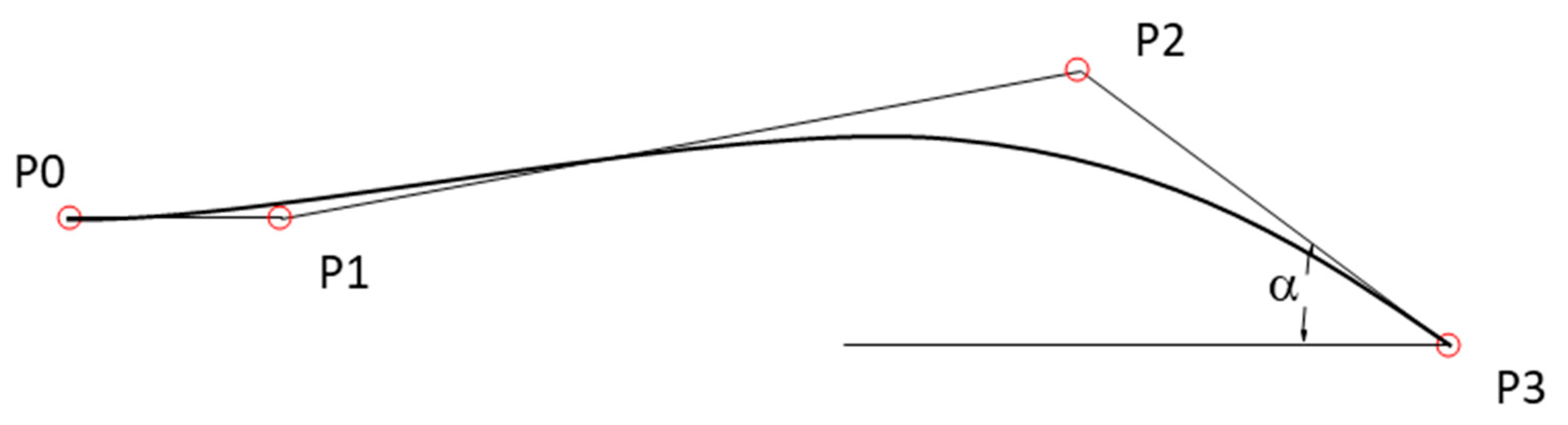
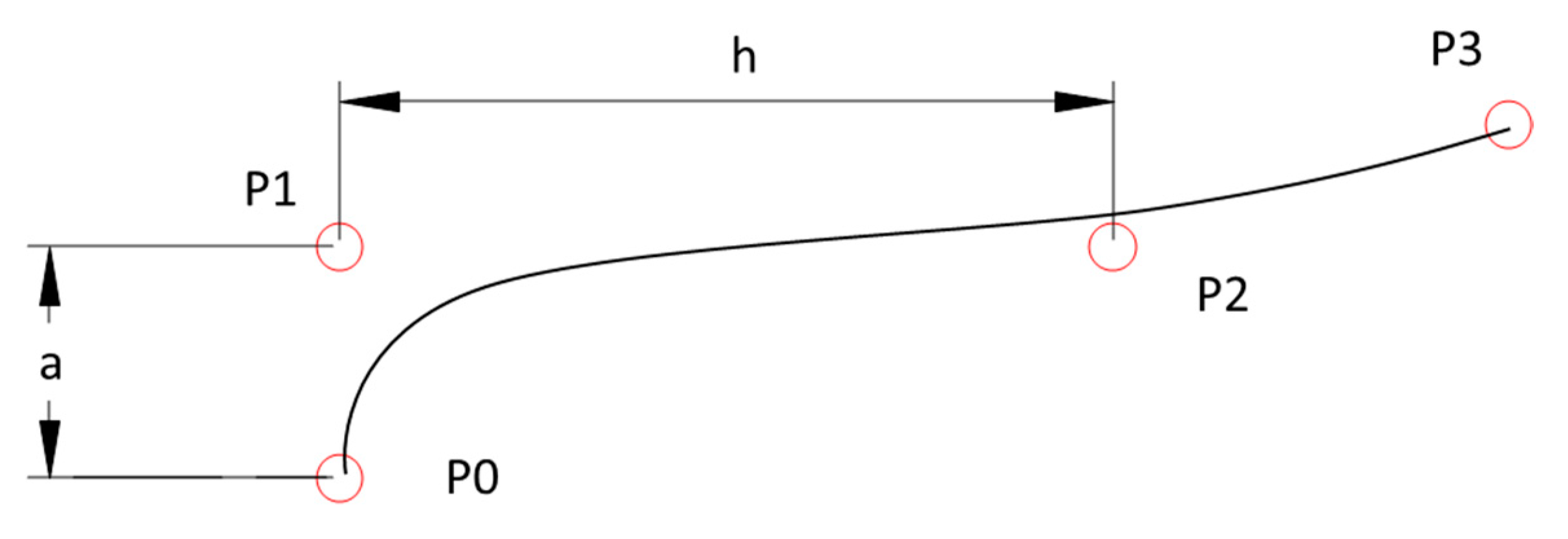
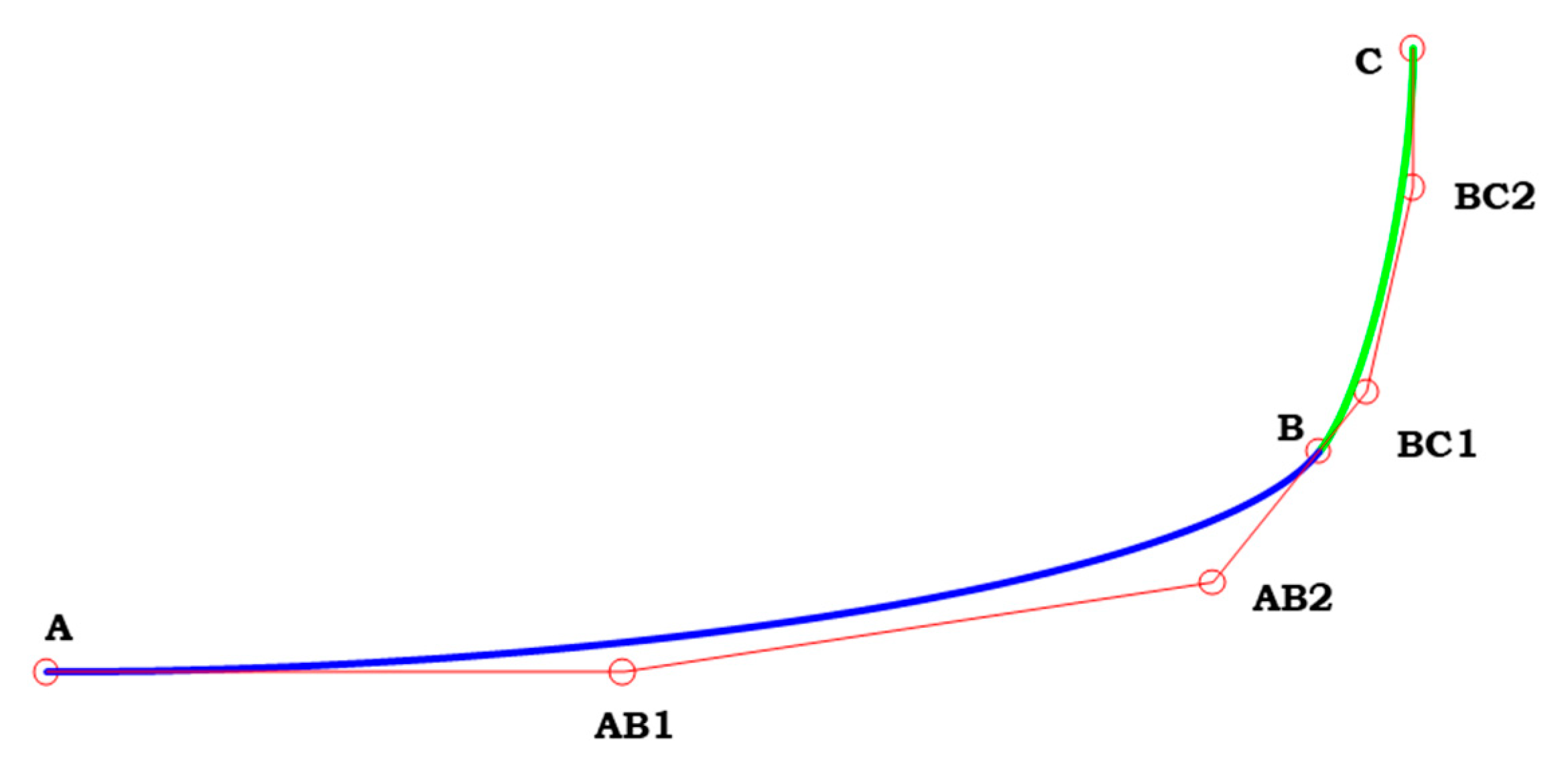
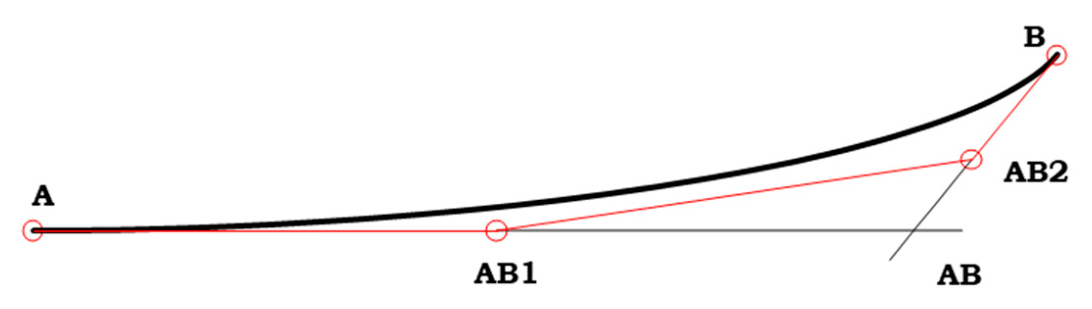
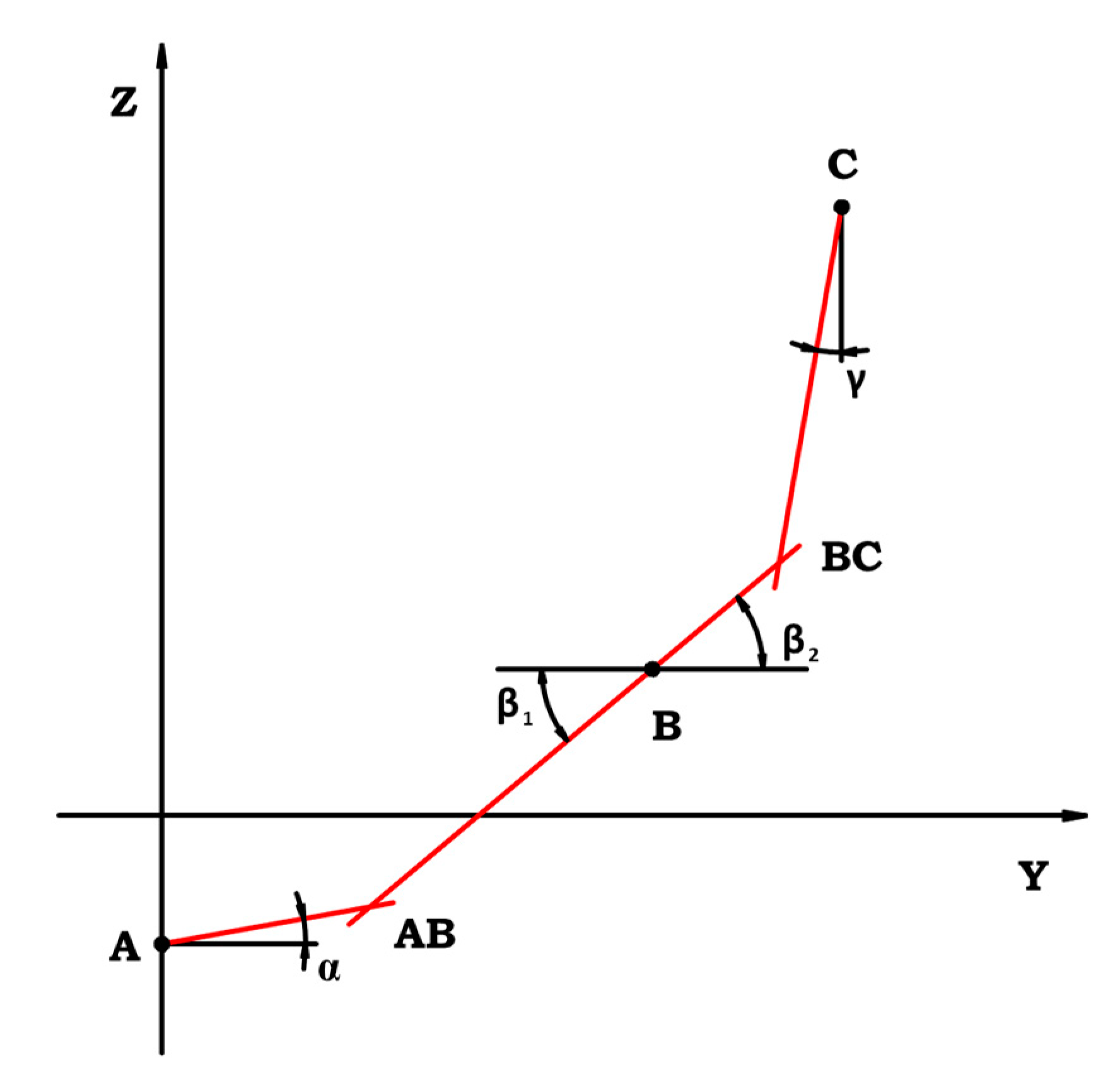
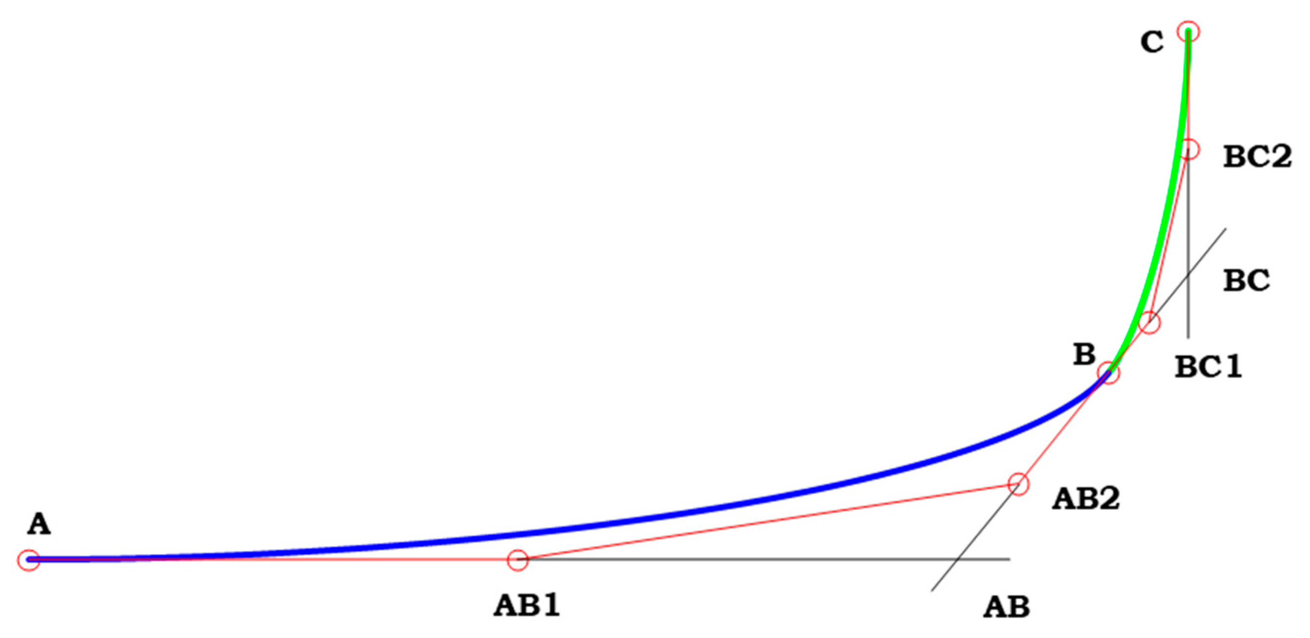
2. Rational Bézier Curves

The rational Bézier curves are a particular family of the Bézier curves as presented in [19]. They can be described with the following Equation (1).

$$C\left(t\right)=\frac{{{\displaystyle \sum }}_{i=0}^n{w}_i{B}_{i,n}\left(t\right)P_i}{{{\displaystyle \sum }}_{i=0}^n{w}_i{B}_{i,n}\left(t\right)},t=0,\dots ,1$$

(1)

where n is the order of the curve, P_i and w_i are the control points and the weights respectively, while B_i,n(t) are the Bernstein polynomials defined over the parametric abscissa t and described by the following Equation (2).

$$B_{i,n}\left(t\right)=\frac{n!}{i!\left(n-i\right)!}{t}^i{\left(1-t\right)}^{n-i},\hspace{1em}i=0,1,\dots ,n,$$

(2)

The principal difference between a rational Bézier curve and a classic one consists in the possibility of modifying the shape of a given curve without moving the control points. This is possible thanks to the weights assigned to each control point. In this way the designer can manipulate the shape of the curve and maintain the order of continuity in the ending points in terms of tangency and curvature. Being these curves tangent to the control polygon at the endpoints, the designer can have direct control on the initial and final angle of tangency of the curve. An example of this property is shown in Figure 1.

Regarding the control of the curvature $\left(\mathit{k}\right)$ at the ending points there is another important property of the rational Bézier curves that allows the designer to link the position and weights of the control points to the value of the curvature. This relation is presented in the next Equation (3).

$$k\left(t_0\right)=\frac{w_0{w}_2}{w_1^2}\frac{n-1}{n}\frac{h}{a^2},$$

(3)

where n is the order of the curve, w_i are the weights of the control points while a and h are defined in Figure 2.

A practical application of these two properties can be seen in the following example. In Figure 3 two rational Bézier curves sharing the common point B are plotted.

The curve resulting from the union of these two curves presents a continuity of the second order. As it is possible to observe in Figure 3, the ending point of the blue curve is coincident with the starting point of the green curve (G0 = C0 continuity) and points AB2, B and BC1 are all aligned (G1 continuity). Regarding the curvature (G2 continuity), the designer can apply Equation (3) to establish that the curvature of the green curve is the same as the curvature of the blue curve calculated in point B (or vice-versa). To achieve this condition the designer can first calculate the value of the curvature in point B of the blue curve using Equation (3), then with the following Equation (4) calculate the value to assign to the weight of the control point BC1 to match the same value of the curvature of the blue curve and the green curve in their common point.

$$w_{BC1}=\sqrt{\frac{2}{3}\frac{w_B{w}_{BC2}}{k\left(B\right)}\frac{h}{a^2}}.$$

(4)

Another interesting property of the rational Bézier curves consists of the possibility of increasing the degree of the curve without modifying the shape of the curve itself. In Figure 4 is shown an example of this property.

The original (quadratic) curve is defined by three points A, AB and B. To obtain the corresponding cubic curve the designer can apply the following procedure:

$$\begin{gathered} X_A{}^{*}=X_A \\ {Y}_A{}^{*}=Y_A \\ {X}_{AB1}{}^{*}=\frac{X_A}{3+\frac{2}{3}{X}_{AB}} \\ {Y}_{AB1}{}^{*}=\frac{Y_A}{3+\frac{2}{3}{Y}_{AB}} \\ {X}_{AB2}{}^{*}=\frac{2}{3}{X}_{AB}+\frac{X_B}{3} \\ {Y}_{AB2}{}^{*}=\frac{2}{3}{Y}_{AB}+\frac{Y_B}{3} \\ {X}_B{}^{*}=X_B \\ {Y}_B{}^{*}=Y_B, \end{gathered}$$

(5)

where the coordinates marked with * are representative of the new curve. The new curve is defined with four control points, A, AB1, AB2 and B, resulting in a higher degree curve compared to the starting one.

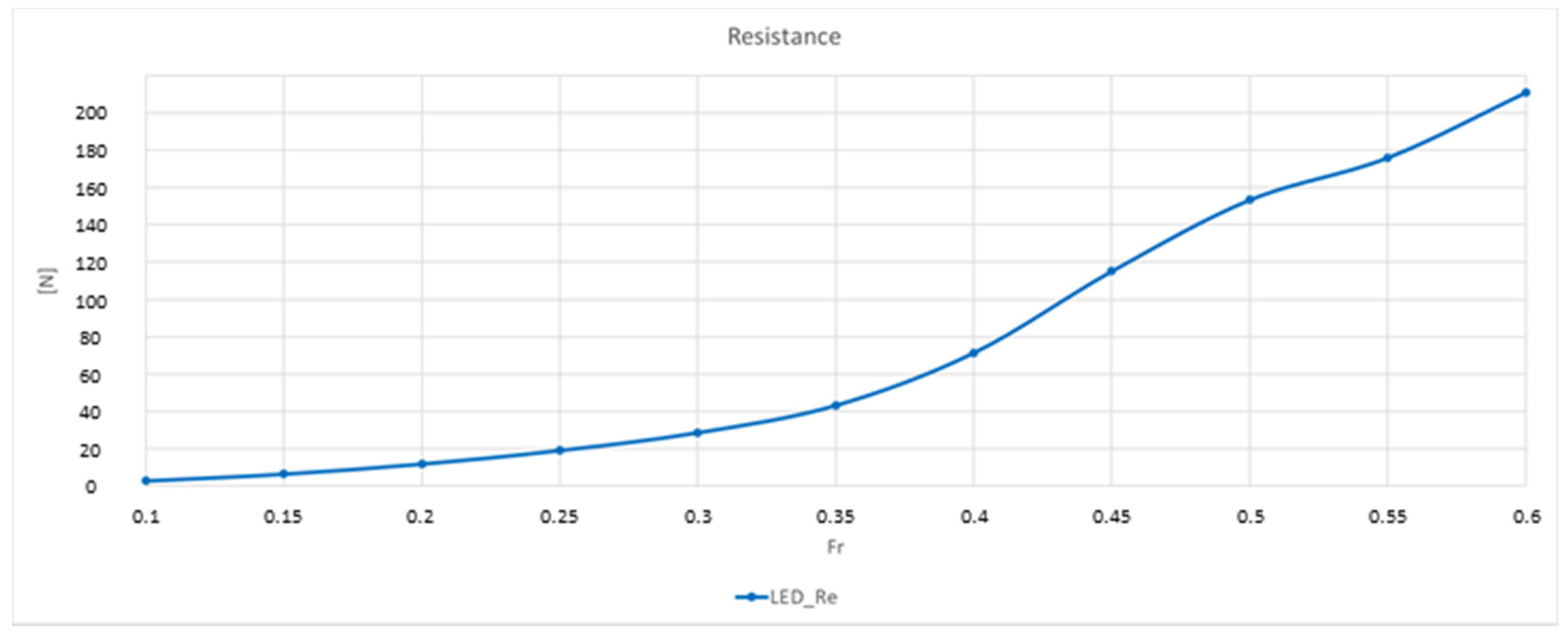
3. Estimation of Resistance for a Sailboat

Since 1975, researchers interested in sailing have been developing regression curves based on polynomial expressions with the aim of estimating the resistance of the hull of a sailboat. Nowadays there are several approaches to evaluate the resistance curve of a sailboat; one of the most common is the formulation proposed by [11] and the updated version presented in [12]. Both the formulations are based on the experimental campaign conducted at the Delft Ship Hydromechanics Laboratory of the Delft University of Technology. For the purpose of this work the older formulation has been preferred since in [12] typical coefficients concerning maxi yachts and higher Froude number are taken into account. Equation (6) shows the regression formulation for the estimation of the residuary resistance, Rrh, of the bare hull whose applicability ranges between Fr 0.10 and 0.60 stepped by 0.05.

$$\begin{gathered} \frac{Rrh}{\nabla c·\rho ·g}=a_0+\left(a_1·\frac{LC{B}_{fpp}}{Lwl}+a_2·Cp+a_3·\frac{\nabla c^{\frac{2}{3}}}{Aw}+a_4·\frac{Bwl}{Lwl}\right)·\frac{\nabla c^{\frac{1}{3}}}{Lwl}+ \\ +\left(a_5·\frac{\nabla c^{\frac{2}{3}}}{S_W}+a_6·\frac{LC{B}_{fpp}}{LC{F}_{fpp}}+a_7·{\left(\frac{LC{B}_{fpp}}{Lwl}\right)}^2+a_8·C{p}^2\right)·\frac{\nabla c^{\frac{1}{3}}}{Lwl}. \end{gathered}$$

(6)

The coefficient a_i In Equation (6), can be found in reference [11], while in the Nomenclature section the meaning of the parameters are defined. To obtain the total hull resistance it is also necessary to compute the component of the resistance due to friction. In Equation (7) there is one of the possible empirical formulation widely used by the researchers [5] to define the friction coefficient.

$$c_f=\frac{0.075}{{(\log \left(Re\right)-2)}^2}.$$

(7)

Consequently, the friction resistance can be expressed with the well-known equation:

$$R_f=\frac{1}{2}\rho v^2{S}_w{c}_f.$$

(8)

The sum of the resistances estimated in Equations (6) and (8) permits to obtain the total resistance of the bare hull of a sailboat, as shown in Equation (9).

$$R=Rrh+R_f.$$

(9)

4. Design Approach

In this work, quadratic and cubic rational Bézier curves, whose formulation has been presented in Section 2, are used to design a sailboat. The shape of the hull is defined by three sections (fore, mid and aft), three longitudinal curves (sheer, chine and keel) and the right ahead. In this way, the whole domain is divided into three parts, as can be seen in Figure 5 where the red circles represent the intersection of the curves. In this way, the design variables of the problem are the Cartesian coordinates of the control points (the red circles) and the tangency of the curves at their ends.

Sections are defined with rational Bézier curves of second or third-degree depending on the type of the boat, respectively hard-chine or round-bilge. Each section is composed of two curves—one starting from the keel ending to the chine and the second one starting from the chine ending to the sheer. In this way, it is possible to generate a wide range of shapes. In Figure 6 the structure of the sections of a round-bilge hull is presented.

To properly define the shape of all the curves of Figure 5, the designer can insert the values of the coordinates of the control points of the curves with the help of a user-interface as shown in the following Figure 7 and Figure 8. The definition of the curves by means of the rational Bézier formulation is particularly suitable for the design of the hull of a sailboat. In fact, once the main dimensions have been defined (e.g., max beam, max draught, length of water line), the designer can adjust the fullness of each curve without modifying the control polygon but just acting on the weights of the control points or the tangency at their ends.

To assure G0 continuity of the section, the position of the control points of the two curves at the chine have to be coincident. G0 continuity is enough for a hard-chine sailboat. While for a round-bilge sailboat, G1 and G2 continuity have to be imposed as well. G1 continuity can be obtained by controlling the tangency of the curves in the common point B lying on the chine (angles β₁ and β₂ in Figure 9). So, in the case of hard-chine β₁ ≠ β₂, while in the case of round-bilge β₁ = β₂.

As can be seen the control points AB, B and BC are all lying in the same line so the angle at the end of the first curve is the same as the starting angle of the second curve and G1 continuity is respected. To assure the G2 continuity, the second-degree curve is not sufficient so, as presented in Section 2, the curve is automatically modified to obtain a third-degree curve using Equation (5), then Equations (3) and (4) are applied to impose the same curvature at the common point of the two curves (point B). In Figure 10 the new control polygon assuring G2 continuity of a section is shown.

Once all the curves have been defined, the Visual Basic for Application (VBA) tool prints several exchange files with the information of each curve following two different strategies. In the first one each curve is sampled in a fixed number of points and their coordinates (in ASCII format) can be imported in several CAD software that re-creates the curves by interpolating these points. In the second format, each curve is defined with the syntax form of an IGES file [20] preserving, in this way, its mathematics. According to the latter method, a macro has been set up in the parametric software CREO 4.0 from PTC aimed to import all the curves and automatically generate the sweep surface of the whole hull. Figure 11 shows the surface of a round-bilge sailboat.

Now the designer can have a closer look to the curves and surface using all the feature of a commercial CAD software. For instance, Figure 12 shows a screenshot of the gaussian curvature of a hard-chine hull.

Still inside CREO 4.0 the coefficients used in Equation (6), whose definition is given in the Nomenclature section, are automatically calculated. The VBA tool grasps these information and evaluates the resistance curve of the specific hull vs. the Froude number [11], plotting the results as shown in Figure 13.

5. Design an Existing Sailboat

In this section two existing sailboats are replicated to validate the method presented in Section 4. The type of sailboat selected are the so called SKIFF (Sail Keep It Flat and Fast) shown in Figure 14 that take part to the international annual regatta 1001Velacup® held in Italy every year in September.

These two boats, although quite similar in terms of displacement, length and main parameters, are characterized by a different hull shape. LED is a classical round-bilge, designed to sail at a low Froude number while TryAgain is a hard-chine hull, mainly designed for sail at a higher Froude number. In Figure 15 the designs of both the hulls are shown (LED on the top and TryAgain on the bottom).

Applying the method presented in Section 4, the two hulls were replicated. In particular, Figure 16 shows the overlap of the original and rebuilt curves, while Figure 17 shows the cut-off of the rebuilt surfaces modelled as previously said in CREO 4.0 with transversal planes to show the sections (red curves), with horizontal planes to show the waterlines (blue curves) and with longitudinal planes to show the buttocks (green curves). A well faired curves frame has been obtained without undesired changes in slope or curvature confirming the goodness of the proposed approach.

Once the geometry of the hulls has been defined, the main characteristics of the two sailboats are automatically calculated.

Table 1. Coefficients of the original and rebuild hulls.

Entity	Symbol	Unit	LED		TryAgain
			Original	Rebuilt	Original	Rebuilt
Displacement	∇	m3	0.257	0.258	0.262	0.263
Length Overall	LOA	m	4.60	4.60	4.60	4.60
Length Water Line	LWL	m	4.46	4.46	4.49	4.49
Max Beam Water Line	BWL	m	1.05	1.05	0.95	0.95
Wetted Surface	SW	m2	3.49	3.48	3.46	3.50
Water Plane Area	AW	m2	3.21	3.20	3.10	3.14
Max Transversal Area	AX	m2	0.107	0.107	0.094	0.093
Long. Centre of Buoyancy	LCB	m	2.48	2.52	2.25	2.26
Long. Centre of Flotation	LCF	m	2.69	2.70	2.60	2.60
Max Draught	Tc	m	0.14	0.14	0.17	0.17
Prismatic Coefficient	Cp		0.539	0.540	0.621	0.629
Midship Section Coefficient	Cm		0.728	0.728	0.582	0.576

shows the comparison of the main hull characteristics whose definitions can be found in [5].

As can be seen in the previous table, also the differences in terms of coefficients are very narrow so the method results effectively to replicate a sailboat. In addition, the resistance curves have been calculated with the procedure presented in Section 3 and in Figure 18 the original and rebuilt hulls are compared. It is evident that the rebuild process does not affect the performance prediction: the resistance curves of both the hulls are completely overlapped, and no appreciable differences can be observed. Some basic comments about this plot can be done as follows: differences between the two hulls can be appreciated in the range Fr = [0.25–0.4] where LED has lower resistance than TryAgain and in the range Fr = [0.4–0.55] where the opposite happens. This is mainly due to the performance characteristic of the round bilge (LED) and of the hard chine (TryAgain): at low speed, faired streamlines are favored by the smoothness of the round bilge reducing the friction resistance; at higher speed, lifting forces generated by the hard chine enhance pre-planing phenomena and, as a consequence, a reduced wave resistance [5].

6. Design of a New Sailboat

As can be seen in Figure 18, depending on the sailing conditions, LED or TryAgain is better than the other one. To understand the reasons for these differences in terms of the resistance of the two hulls, an investigation on the effect of the coefficients on the computed resistance was carried on. In

Table 2. Comparison between the coefficients of LED and TryAgain.

Coeff.	LED	TryAgain	Diff. (%)
VC	0.258	0.263	+1.90
LCB	2.47	2.26	−9.29
SW	3.48	3.50	+0.57
LWL	4.46	4.49	+0.67
BWL	1.05	0.95	−10.53
AW	3.20	3.14	−1.91
LCF	2.70	2.60	−3.85
TC	0.14	0.17	+17.65
AX	0.107	0.093	−15.05
CP	0.540	0.629	+14.15
CM	0.728	0.576	−26.39

the coefficients of LED and TryAgain are compared to see which one is the most different. The last column reports the difference (Coeff_TryAgain − Coeff_LED)/Coeff_LED.

As can be seen in the previous table, the largest differences in terms of coefficients of the two sailboats are the Longitudinal Centre of Buoyancy (LCB), the Beam of the Water Line (Bwl), the Max Draught (Tc) and the Max Transversal Area (Ax).

VPP is very sensitive to slight changes of the coefficients. In particular, there are appreciable differences in terms of resistance starting from Froude 0.4, since for lower ranges of Froude number the biggest quote to the resistance is related to friction. Reducing the value of LCB causes better performances for medium speeds, reducing BWL generates a sailboat that performs in a better way at high Froude numbers, reducing T_C and A_X have a not optimal resistance trend for low values of Froude numbers but on the other hand good one for high Froude numbers.

The goal is to obtain a new shape that has the advantages of the two hulls LED and TryAgain. To reach this objective the new hull should have a low B_WL and a low C_P in order to preserve the performances of LED at a low Froude number; at the same time, this new hull should need a hard-chine to preserve the performances of TryAgain at higher Froude number. As a matter of course, reducing the value of B_WL will lead to having a higher T_C to match the total displacement of the sailboat.

With all this information, the authors started an intensive campaign to obtain a new sailboat. The approach can be considered heuristic and knowledge-based with the goal of obtaining a new hull design as similar as possible to LED, with good performances at low values of Froude numbers, but with a chine to take advantage of its positive effect at high values of Froude numbers. After several attempts using the approach here presented a new design was defined and the obtained lines are shown in Figure 19 while in

Table 3. Comparison of the coefficients of LED, TryAgain and LED_UP_06.

Coeff.	LED	TryAgain	LED_UP_06
VC	0.258	0.263	0.259
LCB	2.47	2.26	2.48
SW	3.48	3.50	3.39
LWL	4.46	4.49	4.48
BWL	1.05	0.95	0.995
AW	3.20	3.14	3.08
LCF	2.70	2.60	2.71
TC	0.14	0.17	0.16
AX	0.107	0.093	0.107
CP	0.540	0.629	0.540
CM	0.728	0.576	0.689

the coefficients of the three sailboats are compared.

In Figure 20 the surface of the new hull is generated and cut off with transversal planes to show the sections (red curves), with horizontal planes to show the waterlines (blue curves) and with longitudinal planes to show the buttocks (green curves).

Finally, applying the method presented in Section 3, the resistance curves of the three hulls are compared and the result plotted in Figure 21.

As can be seen in the previous figure, the VPP indicates that LED_UP_06 is the best hull in light wind condition (low Froude number), then TryAgain gains advantage for medium ranges of speed, followed by LED_UP_06.

To resume, in Figure 22, the resistances calculated for LED and TryAgain have been compared to the ones calculated for LED_UP_06. The blue areas indicate where and how much LED_UP_06 is better than the original hulls, while the red areas indicate the opposite. The green line compares LED with LED_UP_06 and the area below this line is always blue in the analyzed Fr range. This means that the new hull guarantees better performances with respect to LED at any Fr. The red line compares TryAgain with LED_UP_06 and the areas below this line are red or blue depending on the value of Fr. Basically, LED_UP_06 behaves better than TryAgain in the range Fr = [0.21–0.4] and the improvements arrive at the 9% of the resistance. TryAgain has lower values of resistance for medium-high values of Froude number (Fr > 0.4), which is a consolidated result in literature since a higher value of C_P leads to better performances in this range of speeds. Nevertheless, the better performance due to the pre-planing attitude shown by TryAgain at high Fr can become significant in the choice between the two hulls only when high speed is assumed during regattas. Usually these competitions are held in light breeze conditions and rarely boats are fully planing. Moreover, frequent restarts of the boat due to maneuvering require a boat able to quickly accelerate and in this sense, the low resistance shown by LED_UP_06 at medium Fr range could be of great importance.

7. Conclusions

In this work, a tool and the relative methodology to design and evaluate the performances of hulls of sailing boats is presented. The algorithm and the related Graphical User Interface (GUI) have been written in Visual Basic for Excel. A total of seven rational Bézier curves of the third-degree are selected to define the geometry of the hull. To prove the validity of the tool and the applied approach, two existing sailboat hulls have been successfully replicated and a new design of a sailboat is presented.

This procedure has been used to rapidly design a new hull that includes benefits given by a round bilge and a hard chine hull. It has been demonstrated that a hybrid solution between these two opposite shapes ensures better performance especially in the mid-range of Fr, before lifting effects on the hull due to dynamic pressure prevail.

In future works the new hull will be investigated by means of CFD simulations, in a wider range of real sailing conditions in terms of Froude number, trim and leeway angles, allowing the designer to understand in a deeper way why the hulls present differences in terms of performances.

References

1. Nam, J.; Bang, N.S. A curve based hull form variation with geometric constraints of area and centroid. Ocean Eng. 2017. [Google Scholar] [CrossRef]
2. Khan, S.; Gunpinar, E.; Sener, B. GenYacht: An interactive generative design system for computer-aided yacht hull design. Ocean Eng. 2019. [Google Scholar] [CrossRef]
3. Cirello, A.; Cucinotta, F.; Ingrassia, T.; Nigrelli, V.; Sfavara, F. Fluid-structure interaction of downwind sails: A new computational method. J. Mar. Sci. Technol. 2019, 24, 86–97. [Google Scholar] [CrossRef]
4. Mancuso, A. Parametric design of sailing hull shapes. Ocean Eng. 2006, 33, 234–246. [Google Scholar] [CrossRef]
5. Larsson, L.; Eliasson, R.E.; Orych, M. Principles of Yacht Design; Adlard Coles Nautical: London, UK, 2014. [Google Scholar]
6. Calkins, D.E.; Schachter, R.D.; Oliveira, L.T. An automated computational method for planning hull form definition in concept design. Ocean Eng. 2001, 28, 297–327. [Google Scholar] [CrossRef]
7. Chrismianto, D.; Zakki, A.F.; Arswendo, B.; Kim, D.J. Development of Cubic Bezier Curve and Curve-Plane Intersection Method for Parametric Submarine Hull Form Design to Optimize Hull Resistance Using CFD. J. Mar. Sci. Technol. 2015, 14, 399–405. [Google Scholar] [CrossRef] [Green Version]
8. Khan, S.; Gunpinar, E.; Dogan, K.M. A novel design framework for generation and parametric modification of yacht hull surfaces. Ocean Eng. 2017. [Google Scholar] [CrossRef] [Green Version]
9. Pérez-Arribas, F. Parametric generation of planing hulls. Ocean Eng. 2014, 81, 89–104. [Google Scholar] [CrossRef]
10. Ingrassia, T.; Mancuso, A.; Nigrelli, V.; Tumino, D. A multi-technique simultaneous approach for the design of a sailing yacht. Int. J. Interact. Des. Manuf. 2017, 11, 19–30. [Google Scholar] [CrossRef]
11. Keuning, J.A.; Sonnenberg, U.B. Approximation of the hydrodynamic forces on a sailing yacht based on the Delft Systematic Yacht Hull Series. In Proceedings of the 15th International Symposium on “Yacht Design and Yacht Construction”, Amsterdam, The Netherlands, 16 November 1998; ISBN 902700171-8. [Google Scholar]
12. Keuning, J.A.; Katgert, M. A bare hull resistance prediction method derived from the results of the Delft systematic yacht hull series extended to higher speeds. In Proceedings of the International Conference on Innovation in High Performance Sailing Yachts, Lorient, France, 29–30 May 2008. [Google Scholar]
13. Savitsky, D.; Brown, P.W. Procedures for Hydrodynamic Evaluation od Planing Hulls in Smooth and Rough Water. Mar. Technol. 1976, 13, 381–400. [Google Scholar]
14. ITTC. Practical Guidelines for Ship CFD Applications. In Proceedings of the 26th International Towing Tank Conference, Rio de Janeiro, Brazil, 28 August–3 September 2011. [Google Scholar]
15. ITTC. Uncertainty Analysis in CFD Verification and Validation Methodology and Procedures. In Proceedings of the Recommended Procedures and Guidelines of the International Towing Tank Conference; 2017. Available online: https://www.ittc.info/media/7691/75-04-01-011.pdf (accessed on 26 March 2021).
16. Eca, L.; Hoekstra, M. A procedure for the estimation of the numerical uncertainty of CFD calculations based on grid refinement studies. J. Comput. Phys. 2014, 262. [Google Scholar] [CrossRef]
17. Raymond, J.; Cudby, K. Using Parametric Modelling, CFD, and Historical Data, to Estimate Planing Hull Performance on a Laptop. In Proceedings of the 4th High Performance Yacht Design Conference, Auckland, New Zealand, 12–14 March 2012. [Google Scholar]
18. Viola, I.M.; Enlander, J.; Adamson, H. Trim effect on the resistance of sailing planing hulls. Ocean Eng. 2014, 88, 187–193. [Google Scholar] [CrossRef] [Green Version]
19. Sederberg, T.W. Computer Aided Geometric Design. Computer Aided Geometric Design Course Notes; BYU Scholars Archive, 2012; Available online: https://scholarsarchive.byu.edu/cgi/viewcontent.cgi?article=1000&context=facpub (accessed on 26 March 2021).
20. ANSI Standard. Initial Graphics Exchange Specification IGES 5.3; U.S. Product Data Association: Charleston, SC, USA, 1996. [Google Scholar]
Figure 1. Tangency at the end points of a Bézier curve.
Jmse 09 00360 g001
Figure 2. Curvature at the end points of a rational Bézier curve.
Jmse 09 00360 g002
Figure 3. Two rational Bézier curves with a point in common.
Jmse 09 00360 g003
Figure 4. Degree elevation of a rational Bézier curve.
Jmse 09 00360 g004
Figure 5. Curves frame used to define the hull surface.
Jmse 09 00360 g005
Figure 6. Structure of the curve of a section of the hull.
Jmse 09 00360 g006
Figure 7. User-interface of a section.
Jmse 09 00360 g007
Figure 8. User-interface of the sheer, chine and keel lines.
Jmse 09 00360 g008
Figure 9. Control polygon of a G1 second-degree rational Bézier curve.
Jmse 09 00360 g009
Figure 10. Section modeled with a G2 third-degree rational Bézier curve.
Jmse 09 00360 g010
Figure 11. Surface model of a sailboat designed in CREO 4.0 with the information from the VBA tool.
Jmse 09 00360 g011
Figure 12. Curvature analysis of the surface of the hull.
Jmse 09 00360 g012
Figure 13. Resistance curve of the hull of a sailboat.
Jmse 09 00360 g013
Figure 14. The Sail Keep It Flat and Fast (SKIFF) LED and TryAgain during the regattas of 2013 in La Spezia, Italy.
Jmse 09 00360 g014
Figure 15. Hull design of LED (top) and TryAgain (bottom).
Jmse 09 00360 g015
Figure 16. Lines of the original hulls (black) and rebuilt ones (red). LED on the left part and TryAgain on the right (part).
Jmse 09 00360 g016
Figure 17. Rebuilt hull surfaces: LED (left) and TryAgain (right).
Jmse 09 00360 g017
Figure 18. Resistance curves of the original and rebuild hulls.
Jmse 09 00360 g018
Figure 19. The lines of the new design.
Jmse 09 00360 g019
Figure 20. Surface of LED_UP_06.
Jmse 09 00360 g020
Figure 21. Comparison between the resistance curves of LED, TryAgain and LED_UP_06.
Jmse 09 00360 g021
Figure 22. Difference in percentage between LED and LED_UP_06 and TryAgain and LED_UP_06.
Jmse 09 00360 g022