L2-Gain-Based Practical Stabilization of an Underactuated Surface Vessel

Abstract

To obtain a stabilizer for an underactuated surface vessel with disturbances, an L2-gain design is proposed. Surge, sway, and yaw motions are considered in the dynamics of a surface ship. To ob-tain a robust adaptive controller, a diffeomorphism transformation and the Lyapunov function are employed in controller design. Two auxiliary controllers are introduced for an equivalent sys-tem after the diffeomorphism transformation. Different from the commonly used disturbance ob-server-based approach, the L2-gain design is used to suppress random uncertain disturbances in ship dynamics. To evaluate the controller performance in suppressing disturbances, two error sig-nals are defined in which the variables to be stabilized are incorporated. Both time-invariant dis-continuous and continuous feedback laws are proposed to obtain the control system. Stability analysis and simulation results demonstrate the validity of the controllers proposed. A comparison with a sliding mode controller is performed, and the results prove the advantage of the proposed controller in terms of faster convergence rate and chattering avoidance.

1. Introduction

Marine vessels are usually underactuated systems, which implies a lack of an actuator at some degree of freedom. A representative example is the absence of side-thruster in most surface vessels, which are typically equipped with a main thruster and rudder at the stern. As a result, the surge motion and yaw motion of the surface vessel can be controlled directly, while the sway motion cannot be controlled directly. This underactuation creates challenges for the guidance and control of surface vessels. The control systems designed for fully actuated vessels cannot be directly employed to underactuated systems since the resulting performance is very poor [1]. During the last decades, continuous attention has been paid to the control of underactuated surface vessels (USVs), including stabilization, path following, trajectory tracking, and docking/berthing [2]. Various control strategies have been put forward. In the area of stabilization, since linear and classical nonlinear control theories are not applicable due to the difficulty with Brockett’s theorem [3], two approaches are available for the stabilization of USVs. One is the time-invariant and time-varying discontinuous feedback. For example, a periodic time-varying feedback law was proposed for the stabilization of a USV [4]. A time-invariant discontinuous exponential stabilizer using the σ-process was designed for an underactuated autonomous surface vessel [5]. Robust discontinuous state feedback control laws were proposed for the stabilization of a USV [6]. A time-varying feedback control law including integral action was proposed to stabilize USVs [7]. A time-invariant discontinuous backstepping feedback law was derived to achieve global uniform asymptotic stabilization of a USV [8]. Based on integrator backstepping and time-varying techniques, the global stabilization of a USV was achieved [9]. Based on discontinuous coordinate/input transformations and a Lyapunov-like switching function, a global κ-exponential asymptotic stabilizing law was proposed for USVs [10]. The other approach to the stabilization of USVs is time-varying continuous/smooth feedback. For example, smooth time-varying state backstepping feedbacks were proposed for the global uniform asymptotic stabilization of a USV [11]. By introducing an assistant state variable and a time-varying state transformation, the asymptotic exponential stability of a USV was achieved using a smooth time-varying feedback control law [12]. Three global smooth time-varying control laws were proposed for the stabilization of USVs [13].

From the aforementioned studies, the plant of a USV is assumed to be known exactly, or no uncertainties are considered in the plant, which might degrade the practical feasibility of the controller for stabilization. A representative and inevitable uncertainty for a surface ship moving in sea or waters is the disturbance induced by oceanic environments such as wind, waves, and current. To deal with the uncertainties in the dynamics of USVs, a time-varying feedback control law with a disturbance adaptation law was proposed for an underactuated ship [14]. A global smooth controller in combination with a disturbance observer was presented for the stabilization of an underactuated container ship [15]. A sliding-mode-based stabilizer was designed for a USV with unknown interferences [16]. A smooth time-varying dynamic feedback stabilizer was verified against disturbance torques caused by wind and waves [17]. A transverse function approach was proposed for the practical stabilization of USVs with modeling uncertainties and unknown disturbances [18]. A fuzzy output feedback stabilizer was proposed for a USV with environment disturbances [19].

Generally, the approaches to dealing with a system with external disturbances can be categorized into two types: one aims to suppress disturbance and the other to compensate for disturbance. Most studies on the stabilization of USVs with environmental disturbance compensated for disturbance by designing disturbance observers. The disturbances are often assumed as constants or harmonic signals such as sinusoidal signals. Under this assumption, the disturbances can actually be viewed as certain signals and be dealt with well by disturbance observers. In a sense, such an assumption cannot reflect the uncertain characteristics of environmental disturbances. Different from the disturbance-observer-based approach, the disturbance-suppression-based controller does not require the estimation of disturbance and corresponding compensation but emphasizes the achievement of the required performance associated with the plant even if affected by the worst disturbance. Among disturbance-suppression-based approaches, H_∞ control provides an effective method to suppress uncertain disturbances. As a method of H_∞ control, L2-gain design applies to nonlinear systems with disturbance and has been successfully used in roll stabilization [20,21] and course-keeping [22] of surface vessels. However, the applicability of this method to the stabilization of underactuated surface vessels with disturbances has not received attention. The paper presents an L2-gain approach to the stabilization of a USV affected by random disturbances. An L2-gain design is employed to suppress the disturbances. Since, in most cases, random disturbance is characterized by nonlinearity and uncertainty, it is difficult to precisely estimate these using approximation techniques such as observers, neural networks, and fuzzy logic. L2-gain provides an effective method to obtain a robust controller for a plant under random disturbances. By this method, the influence of disturbance on the required system performance can be suppressed. By appropriately defining the evaluation signals and L2-gain index, controller performance like accuracy and convergence rate can be improved. In the study, the variables to be stabilized are incorporated into the evaluation signals. In addition to the L2-gain design, other techniques adopted in the study include the global diffeomorphism transformation and Lyapunov function method aiming to derive a robust stabilizer. To deal with the underactuation in the plant both time-invariant discontinuous and continuous feedback strategies are employed to guarantee the stabilization of the USV.

The rest of the paper is organized as follows: In Section 2, the mathematical model of the motion of an underactuated surface vessel is given. In Section 3, the controller design process is presented. In Section 4, simulation results based on the proposed controller are reported. Conclusions are given in the final section.

2. Problem Formulations

2.1. Assumptions

In general, the motion of a marine vessel involves six degrees of freedom, as shown in Figure 1a. The coordinate system $o-xyz$ denotes the North-East-Down (NED) reference frame and $o_b-x_{\mathrm{b}}{y}_{\mathrm{b}}{z}_{\mathrm{b}}$ denotes the body-fixed reference frame. Movements including surge, sway, and yaw happen in the horizontal plane while heave, pitch and roll are in the vertical plane [23]. For a surface vessel, the motion in the horizontal plane (i.e., surge, sway, and yaw) is considered, as shown in Figure 1b.

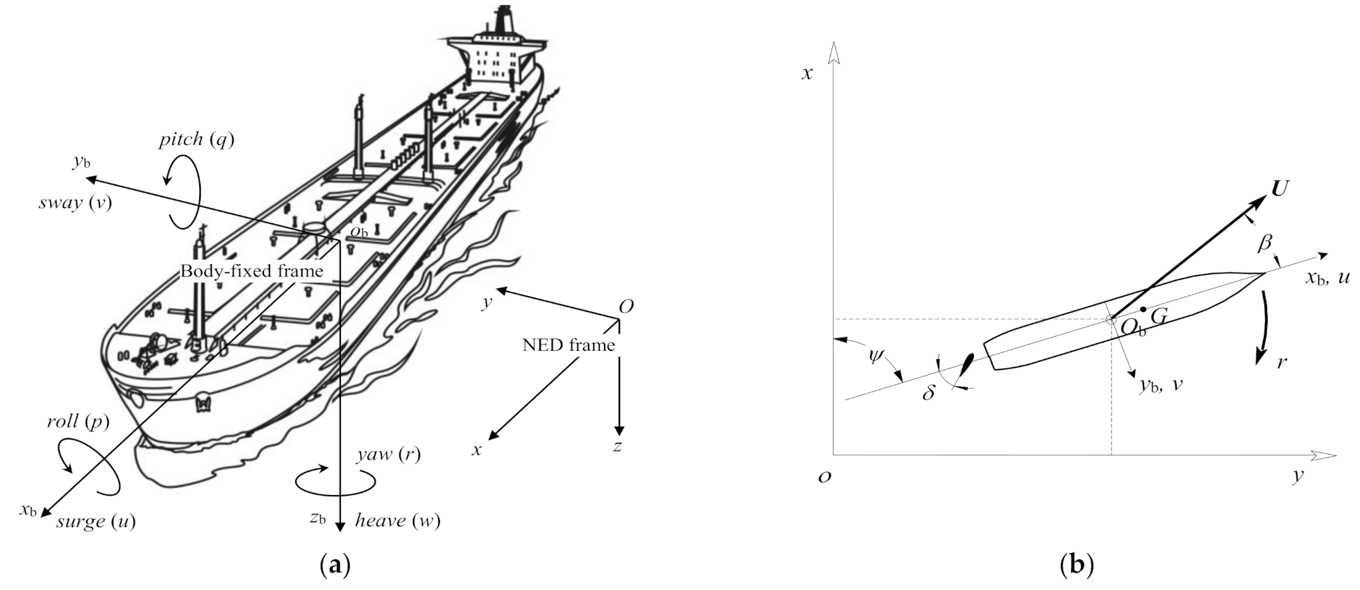
2.2. Mathematical Model

The mathematical model of the dynamics of an underactuated surface ship can be described as

$$\left\{\begin{array}{l}{m}_{11}\dot{u}-m_{22}vr-m_{23}{r}^2+d_{11}u={\tau }_u\\ m_{22}\dot{v}+m_{23}\dot{r}+m_{11}ur+d_{22}v+d_{23}r=0\\ m_{32}\dot{v}+m_{33}\dot{r}+m_{22}vu+m_{23}ru-m_{11}uv+d_{32}v+d_{33}r={\tau }_r\end{array}\right.$$

(1)

where u denotes the surge speed; v is the sway speed, r is the yaw rate. $m_{ij},d_{ij}$ are hydrodynamic coefficients; and ${\tau }_u$ and ${\tau }_r$ are control force and moment impacted on surge motion and yaw motion, respectively. As an underactuated system, there is no actuation in the direction of sway motion.

The kinematics of the ship can be described as

$$\left\{\begin{array}{l}\dot{x}=\left(\cos \psi \right)u-\left(\sin \psi \right)v\\ \dot{y}=\left(\sin \psi \right)u+\left(\cos \psi \right)v\\ \dot{\psi }=r\end{array}\right.$$

(2)

where ψ is the heading angle. (x,y) denotes the coordinate of the ship center. By defining

$$\eta =\left[\begin{array}{c}x\\ y\\ \psi \end{array}\right],\upsilon =\left[\begin{array}{c}u\\ v\\ r\end{array}\right],J(\eta )=J(\psi )=\left[\begin{array}{ccc}\cos \psi & -\sin \psi & 0\\ \sin \psi & \cos \psi & 0\\ 0& 0& 1\end{array}\right],M=\left[\begin{array}{ccc}{m}_{11}& 0& 0\\ 0& m_{22}& m_{23}\\ 0& m_{32}& m_{33}\end{array}\right],$$

$$C(\upsilon )=\left[\begin{array}{ccc}0& 0& c_{13}\\ 0& 0& c_{23}\\ -c_{13}& -c_{23}& 0\end{array}\right],D=\left[\begin{array}{ccc}{d}_{11}& 0& 0\\ 0& d_{22}& d_{23}\\ 0& d_{32}& d_{33}\end{array}\right],\tau =\left[\begin{array}{c}{\tau }_u\\ 0\\ {\tau }_r\end{array}\right],c_{13}=-m_{22}v-m_{23}r,c_{23}=m_{11}u,$$

the mathematical model of the motion of a surface ship can be written as

$$\left\{\begin{array}{l}\dot{\eta }=J(\eta )\upsilon \\ M\dot{\upsilon }+C(\upsilon )\upsilon +D\upsilon =\tau \end{array}\right.$$

(3)

If environmental disturbances are taken into account, the second equation of (3) can be rewritten as

$$M\dot{\upsilon }+C(\upsilon )\upsilon +D\upsilon =\tau +{\tau }_d$$

(4)

where the disturbance term is ${\tau }_d={\left[\begin{array}{ccc}{\tau }_{uw}& {\tau }_{vw}& {\tau }_{rw}\end{array}\right]}^{\mathrm{T}}$.

For systems (1) and (2), by employing a diffeomorphism transformation [1]

$$\left\{\begin{array}{l}\overline{x}=x+\frac{m_{23}}{m_{22}}(\cos \psi -1),\\ \overline{y}=y+\frac{m_{23}}{m_{22}}\sin \psi ,\\ \overline{v}=v+\frac{m_{23}}{m_{22}}r,\end{array}\right.$$

(5)

and controller transformation

$${\tau }_u=m_{11}{\overline{\tau }}_u-m_{22}vr-m_{23}{r}^2+d_{11}u,$$

(6)

$$\begin{array}{c}{\tau }_r=\frac{(m_{22}{m}_{33}-m_{23}{m}_{32})}{m_{22}}{\overline{\tau }}_r-\frac{\left[(m_{11}{m}_{22}-m_{22}^2)uv+(m_{11}{m}_{32}-m_{22}{m}_{23})]ur\right]}{m_{22}}\\ -\frac{\left[(m_{32}{d}_{22}-m_{22}{d}_{32})v-(m_{22}{d}_{33}-m_{32}{d}_{23})r\right]}{m_{22}},\end{array}$$

(7)

We obtain an equivalent system as

$$\left\{\begin{array}{l}\dot{\overline{x}}=u\cos \psi -\overline{v}\sin \psi ,\\ \dot{\overline{y}}=u\sin \psi +\overline{v}\cos \psi ,\\ \dot{\psi }=r,\\ \dot{u}={\overline{\tau }}_u+\frac{1}{m_{11}}{\tau }_{uw},\\ \dot{\overline{v}}=-\alpha ur-\beta \overline{v}+\gamma r+\frac{1}{m_{22}}{\tau }_{vw},\\ \dot{r}={\overline{\tau }}_r+\frac{m_{22}}{(m_{22}{m}_{33}-m_{23}{m}_{32})}{\tau }_{rw}.\end{array}\right.$$

(8)

where the constants $\alpha ,\beta ,\gamma$ are defined as

$$\alpha =\frac{m_{11}}{m_{22}},\beta =\frac{d_{22}}{m_{22}},\gamma =\left(\frac{d_{22}{m}_{23}}{m_{22}^2}-\frac{d_{23}}{m_{22}}\right).$$

If the stability of system (8) can be achieved, i.e., $\underset{t\to \infty }{\lim }\left(\overline{x},\overline{y},\psi ,u,\overline{v},r\right)=0,$ the stability of system (3) can be guaranteed, i.e., $\underset{t\to \infty }{\lim }\left(x,y,\psi ,u,v,r\right)=0$. To make the controller design more direct and systematic, another diffeomorphism transformation is used [11]

$$\left\{\begin{array}{l}{z}_1=\overline{x}\cos \psi +\overline{y}\sin \psi \\ z_2=-\overline{x}\sin \psi +\overline{y}\cos \psi +\frac{1}{\beta }\overline{v}-\frac{\gamma }{\beta }\psi \\ z_3=\psi \\ z_4=-\frac{\alpha }{\beta }u-z_1\\ z_5=\overline{v}\\ z_6=r\end{array}\right.$$

(9)

Similarly, it can be inferred that $\underset{t\to \infty }{\lim }\left(\overline{x},\overline{y},\psi ,u,\overline{v},r\right)=0$ holds if $\underset{t\to \infty }{\lim }\left(z_1,z_2,z_3,z_4,z_5,z_6\right)=0$. The state equation with regard to z_i has the form

$$\left\{\begin{array}{l}{\dot{z}}_1=-\frac{\beta }{\alpha }\left(z_1+z_4\right)+\left(z_2-\frac{1}{\beta }{z}_5+\frac{\gamma }{\beta }{z}_3\right)z_6\\ {\dot{z}}_2=z_4{z}_6+\frac{1}{\beta m_{22}}{\tau }_{vw}\\ {\dot{z}}_3=z_6\\ {\dot{z}}_4=u_1-\frac{\alpha }{\beta m_{11}}{\tau }_{uw}\\ {\dot{z}}_5=-\beta z_5+\beta z_6\left(z_1+z_4\right)+\gamma z_6+\frac{1}{m_{22}}{\tau }_{vw}\\ {\dot{z}}_6=u_2-\frac{m_{32}}{(m_{22}{m}_{33}-m_{23}{m}_{32})}{\tau }_{vw}+\frac{m_{22}}{(m_{22}{m}_{33}-m_{23}{m}_{32})}{\tau }_{rw}\end{array}\right.$$

(10)

where the controllers u₁ and u₂ are defined as

$$u_1=-\frac{\alpha }{\beta }{\overline{\tau }}_u+\frac{\beta }{\alpha }\left(z_1+z_4\right)-z_2{z}_6+\frac{1}{\beta }{z}_5{z}_6-\frac{\gamma }{\beta }{z}_3{z}_6,$$

(11)

$$u_2={\overline{\tau }}_r,$$

(12)

It can be seen from (10) that the state variables $z_2,z_3,z_4,z_6$ depend on the controllers u₁ and u₂ while $z_1,z_5$ do not. Therefore, two subsystems can be defined as

$$\left\{\begin{array}{l}{\dot{z}}_1=-\frac{\beta }{\alpha }\left(z_1+z_4\right)+\left(z_2-\frac{1}{\beta }{z}_5+\frac{\gamma }{\beta }{z}_3\right)z_6\\ {\dot{z}}_5=-\beta z_5+\beta z_6\left(z_1+z_4\right)+\gamma z_6+\frac{1}{m_{22}}{\tau }_{vw}\end{array}\right.$$

(13)

$$\left\{\begin{array}{l}{\dot{z}}_2=z_4{z}_6+\frac{1}{\beta m_{22}}{\tau }_{vw}\\ {\dot{z}}_3=z_6\\ {\dot{z}}_4=u_1-\frac{\alpha }{\beta m_{11}}{\tau }_{uw}\\ {\dot{z}}_6=u_2-\frac{m_{32}}{(m_{22}{m}_{33}-m_{23}{m}_{32})}{\tau }_{vw}+\frac{m_{22}}{(m_{22}{m}_{33}-m_{23}{m}_{32})}{\tau }_{rw}\end{array}\right.$$

(14)

It can be inferred that regardless of controllers u₁ and u₂ are, no asymptotic stability can be achieved for z₂ in subsystem (14) if the disturbance in sway direction, i.e., ${\tau }_{vw}$, does not vanish with time. The same situation happens to z₅ in subsystem (13). In this study it was assumed that ${\tau }_{vw}=0$ while ${\tau }_{uw}$ and ${\tau }_{rw}$ are nonzero. Since there is a close coupling effect between sway motion and yaw motion for surface ships, for simplicity, the disturbance impacted on the sway motion is incorporated into the disturbance in the yaw equation. This way, subsystems (13) and (14) are simplified as

$$\left\{\begin{array}{l}{\dot{z}}_1=-\frac{\beta }{\alpha }\left(z_1+z_4\right)+\left(z_2-\frac{1}{\beta }{z}_5+\frac{\gamma }{\beta }{z}_3\right)z_6\\ {\dot{z}}_5=-\beta z_5+\beta z_6\left(z_1+z_4\right)+\gamma z_6\end{array}\right.$$

(15)

And

$$\left\{\begin{array}{l}{\dot{z}}_2=z_4{z}_6\\ {\dot{z}}_3=z_6\\ {\dot{z}}_4=u_1-\frac{\alpha }{\beta m_{11}}{\tau }_{uw}\\ {\dot{z}}_6=u_2+\frac{m_{22}}{(m_{22}{m}_{33}-m_{23}{m}_{32})}{\tau }_{rw}\end{array}\right.$$

(16)

It has been proven that a stabilizer that is useful for system (16) also guarantees the stability of system (15) [24]. Furthermore, it can be seen that a system consisting of $(z_3,z_6)$ can be decoupled from (16). Two subsystems can be obtained as

$${\mathsf{\Sigma }}_1:\left\{\begin{array}{l}{\dot{z}}_2=z_4{z}_6\\ {\dot{z}}_4=u_1-\frac{\alpha }{\beta m_{11}}{\tau }_{uw}\end{array}\right.$$

(17)

$${\mathsf{\Sigma }}_2:\left\{\begin{array}{l}{\dot{z}}_3=z_6\\ {\dot{z}}_6=u_2+\frac{m_{22}}{(m_{22}{m}_{33}-m_{23}{m}_{32})}{\tau }_{rw}\end{array}\right.$$

(18)

The subsystem Σ₂ is independent of the subsystem Σ₁. Nevertheless, the state variable z₆ exerts an influence on the stability of subsystem Σ₁. To obtain a stabilizer for subsystems Σ₁ and Σ₂, u₂ in the subsystem Σ₂ is designed first. Then u₁ in the subsystem Σ₁ is designed. Afterwards, the control inputs, ${\overline{\tau }}_u$ and ${\overline{\tau }}_r$ in the system (8), can be determined according to (11) and (12). Finally, the control inputs of the original system (1), ${\tau }_u$ and ${\tau }_r$, can be determined according to (6) and (7).

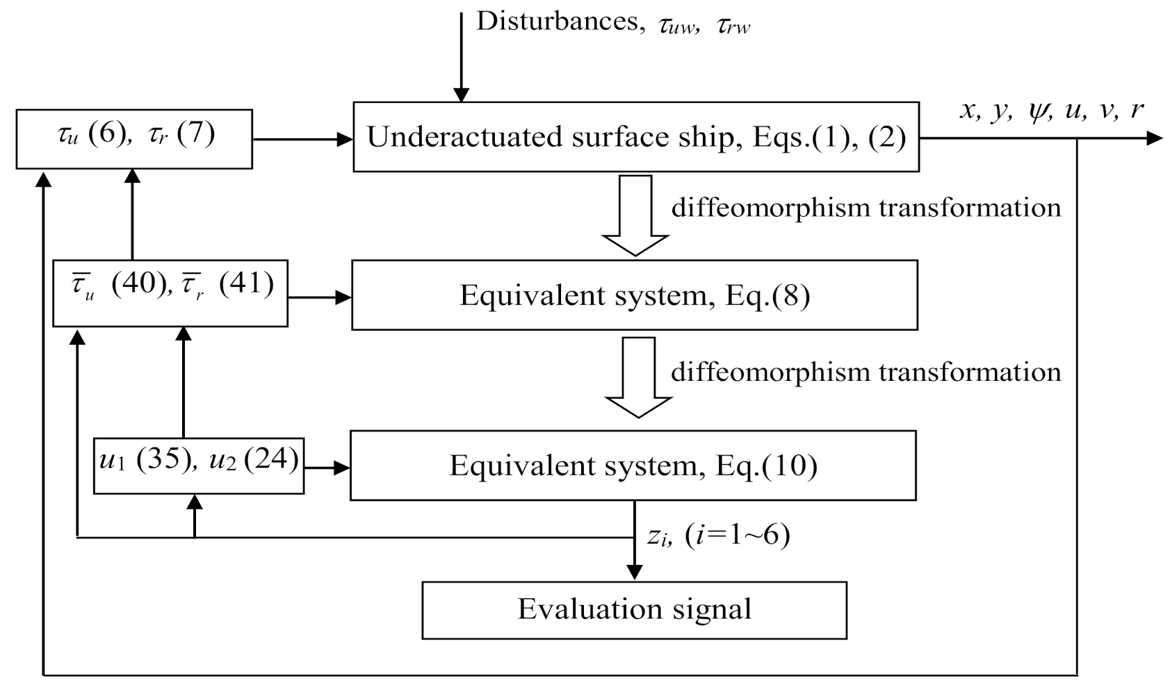
3. Controller Design

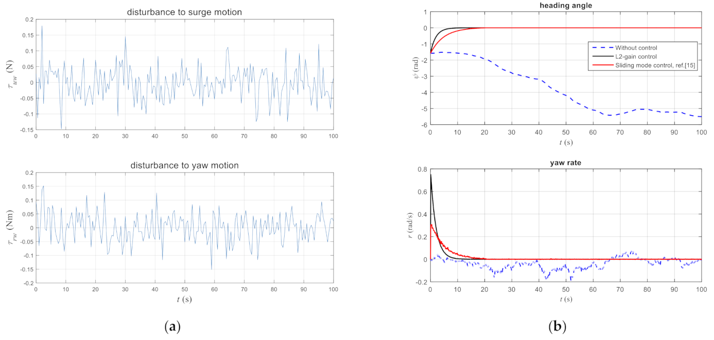
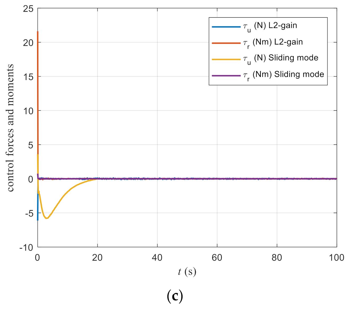
First of all, for subsystem Σ₂, a filtered signal can be defined as

$$\xi =z_6+{\alpha }_1{z}_3,\hspace{0.33em}({\alpha }_1>0).$$

(19)

A Lyapunov function candidate can be defined as

$$V(t)=\frac{1}{2{\lambda }_1}{z}_3^2+\frac{1}{2{\lambda }_1}{\xi }^2$$

(20)

where λ₁ is a positive constant. The time derivative of (20) is

$$\dot{V}=-\frac{{\alpha }_1}{{\lambda }_1}{z}_3^2+\frac{1}{{\lambda }_1}\xi \left(z_3+{\alpha }_1{z}_6+u_2\right)+\xi {{\tau }^{\prime }}_{rw}$$

(21)

where ${{\tau }^{\prime }}_{rw}=\frac{m_{22}}{{\lambda }_1(m_{22}{m}_{33}-m_{23}{m}_{32})}{\tau }_{rw}$.

For a system affected by disturbance, the L2-gain performance of the disturbance suppressing under actuation can be evaluated by [25]

$${\displaystyle {\int }_0^T{‖z‖}^2}dt\le {\gamma }_1^2{\displaystyle {\int }_0^T{‖{{\tau }^{\prime }}_{rw}‖}^2}dt+{\gamma }_0$$

(22)

where $‖\cdot ‖$ represents the Euclidean norm; ${\gamma }_0$ is a positive constant, which is as small as possible. As can be seen in (22), the smaller the ${\gamma }_1$, the smaller the $‖z‖$. If the errors are incorporated into the evaluation signal z, then the errors can become smaller. For system (18), an evaluation signal can be defined as

$$z={\left(\begin{array}{cc}{r}_1{z}_3& r_2\xi \end{array}\right)}^{\mathrm{T}}.\hspace{0.33em}\left(r_1,\hspace{0.33em}{r}_2>0\right)$$

As can be seen, the equality (21) contains the controller u₂ and the disturbance term, ${{\tau }^{\prime }}_{rw}$ while the inequality (22) describes the performance of suppressing the disturbance ${{\tau }^{\prime }}_{rw}$. One can combine (21) with (22) in designing the controller u₂ to guarantee that the inequality (22) holds

$$\begin{array}{c}\dot{V}+{‖z‖}^2-{\gamma }_1^2{{\tau }^{\prime }}_{rw}{}^2=-\frac{{\alpha }_1}{{\lambda }_1}{z}_3^2+\frac{1}{{\lambda }_1}\xi \left(z_3+{\alpha }_1{z}_6+u_2\right)+r_1^2{z}_3^2+r_2^2{\xi }^2+\frac{1}{4{\gamma }_1^2}{\xi }^2-{\left(\frac{1}{2{\gamma }_1}\xi -{\gamma }_1{{\tau }^{\prime }}_{rw}\right)}^2\\ \le \left(r_1^2-\frac{{\alpha }_1}{{\lambda }_1}\right)z_3^2+\frac{1}{{\lambda }_1}\xi \left(\left(1-{\alpha }_1^2\right)z_3+\left({\alpha }_1+{\lambda }_1{r}_2^2+\frac{{\lambda }_1}{4{\gamma }_1^2}\right)\xi +u_2\right)\end{array}$$

(23)

Let the controller u₂ be

$$u_2=-\left(1-{\alpha }_1^2\right)z_3-\left({\alpha }_1+{\lambda }_1{r}_2^2+\frac{{\lambda }_1}{4{\gamma }_1^2}\right)\xi -{\lambda }_1\xi .$$

(24)

The inequality (23) becomes

$$\dot{V}+{‖z‖}^2-{\gamma }_1^2{{\tau }^{\prime }}_{rw}{}^2\le \left(r_1^2-\frac{{\alpha }_1}{{\lambda }_1}\right)z_3^2-{\xi }^2.$$

(25)

By choosing parameters r₁, λ₁, and α₁ to satisfy $r_1^2<\frac{{\alpha }_1}{{\lambda }_1}$, and the right hand side of the inequality (25) can be guaranteed negative, then

$$\dot{V}+{‖z‖}^2-{\gamma }_1^2{{\tau }^{\prime }}_{rw}{}^2\le 0$$

(26)

.

It can be inferred from (26) that, if ${{\tau }^{\prime }}_{rw}=0$ or no disturbance impacted on the plant, $\dot{V}\le 0$ holds, which means the asymptotic stability can be obtained. In the case of ${{\tau }^{\prime }}_{rw}\ne 0$, the goal is to suppress this disturbance or to decrease the influence of disturbance untill inequality (22) is satisfied.

When integrating the inequality (26) from 0 to t, one has

$$V(t)+{\displaystyle {\int }_0^t{‖z‖}^2}\mathrm{d}\tau -{\displaystyle {\int }_0^t{\gamma }_1^2{{\tau }^{\prime }}_{rw}{}^2\mathrm{d}\tau }\le V(0).$$

(27)

furthermore,

$${\displaystyle {\int }_0^t{‖z‖}^2}\mathrm{d}\tau \le {\gamma }_1^2{\displaystyle {\int }_0^t{{\tau }^{\prime }}_{rw}{}^2\mathrm{d}\tau }+V(0).$$

(28)

holds, where

$$V(0)=\frac{1}{2{\lambda }_1}{z}_3^2(0)+\frac{1}{2{\lambda }_1}{\xi }^2(0)$$

(29)

When comparing the above expression with (22), one can define

$${\gamma }_0=V(0)=\frac{1}{2{\lambda }_1}{z}_3^2(0)+\frac{1}{2{\lambda }_1}{\xi }^2(0),$$

(30)

if λ₁ is chosen as a large positive constant. Thus, the performance inequality (22) is satisfied.

For the system Σ₁ expressed by (17), one can define

$$\eta =z_4+{\alpha }_2{z}_2.$$

(31)

A Lyapunov function candidate can be defined as

$$V_1=\frac{1}{2{\lambda }_2}{z}_2^2+\frac{1}{2{\lambda }_2}{\eta }^2$$

(32)

where λ₂ is a positive constant. The time derivative of (32) is

$${\dot{V}}_1=-\frac{{\alpha }_2}{{\lambda }_2}{z}_6{z}_2^2+\frac{1}{{\lambda }_2}\eta \left(u_1+{\alpha }_2{z}_6\left(\eta -{\alpha }_2{z}_2\right)+z_6{z}_2\right)+\eta {{\tau }^{\prime }}_{uw}$$

(33)

where ${{\tau }^{\prime }}_{uw}=-\frac{\alpha }{{\lambda }_2\beta m_{11}}{\tau }_{uw}$.

Similarly, an evaluation signal can be defined as

$$z^{\prime }={\left(\begin{array}{cc}{r}_1{z}_2& r_2\eta \end{array}\right)}^{\mathrm{T}}.$$

Combining the L2-gain with (33) yields

$$\begin{array}{c}{\dot{V}}_1+{‖z^{\prime }‖}^2-{\gamma }_1^2{{\tau }^{\prime }}_{uw}{}^2=-\frac{{\alpha }_2}{{\lambda }_2}{z}_6{z}_2^2+\frac{1}{{\lambda }_2}\eta \left(u_1+{\alpha }_2{z}_6\left(\eta -{\alpha }_2{z}_2\right)+z_6{z}_2\right)+r_1^2{z}_2^2+r_2^2{\eta }^2+\frac{1}{4{\gamma }_1^2}{\eta }^2-{\left(\frac{1}{2{\gamma }_1}\eta -{\gamma }_1{{\tau }^{\prime }}_{uw}\right)}^2\\ \le \left(r_1^2-\frac{{\alpha }_2}{{\lambda }_2}{z}_6\right)z_2^2+\frac{1}{{\lambda }_2}\eta \left(u_1+\left({\lambda }_2{r}_2^2+{\alpha }_2{z}_6+\frac{{\lambda }_2}{4{\gamma }_1^2}\right)\eta +\left(1-{\alpha }_2^2\right)z_6{z}_2\right)\end{array}$$

(34)

Let the controller u₁ be

$$u_1=-\left({\lambda }_2{r}_2^2+{\alpha }_2{z}_6+\frac{{\lambda }_2}{4{\gamma }_1^2}\right)\eta -\left(1-{\alpha }_2^2\right)z_6{z}_2-{\lambda }_2\eta$$

(35)

One has

$${\dot{V}}_1+{‖z^{\prime }‖}^2-{\gamma }_1^2{{\tau }^{\prime }}_{uw}{}^2\le \left(r_1^2-\frac{{\alpha }_2}{{\lambda }_2}{z}_6\right)z_2^2-{\eta }^2$$

(36)

To guarantee the right-hand side of the above inequality negative, the parameter ${\alpha }_2$ can be selected as ${\alpha }_2=\lambda sgn(z_6),\hspace{0.33em}\left(\lambda >0\right)$. By choosing parameters r₁ and λ₂, one has

$${\dot{V}}_1+{‖z^{\prime }‖}^2-{\gamma }_1^2{{\tau }^{\prime }}_{uw}{}^2\le 0$$

(37)

By an analogical analysis referring to (26), the following inequality holds

$${\displaystyle {\int }_0^t{‖z^{\prime }‖}^2}\mathrm{d}\tau \le {\gamma }_1^2{\displaystyle {\int }_0^t{{\tau }^{\prime }}_{uw}{}^2\mathrm{d}\tau }+{{\gamma }^{\prime }}_0.$$

(38)

where

$${{\gamma }^{\prime }}_0=V_1(0)=\frac{1}{2{\lambda }_2}{z}_2^2(0)+\frac{1}{2{\lambda }_2}{\eta }^2(0).$$

(39)

The control system can be depicted as Figure 2. As shown, two equivalent systems can be obtained by means of diffeomorphism transformation. The controller design process starts from the final equivalent system (10) and ends at the original system expressed by (1) and (2). The controllers u₁ and u₂ in the final equivalent system (10) are determined according to (35) and (24) respectively. Afterward, the controllers ${\overline{\tau }}_u$ and ${\overline{\tau }}_r$ in the interim equivalent system (8) can be obtained as

$${\overline{\tau }}_u=\frac{{\beta }^2}{{\alpha }^2}\left(z_1+z_4\right)-\frac{\beta }{\alpha }{z}_2{z}_6+\frac{1}{\alpha }{z}_5{z}_6-\frac{\gamma }{\alpha }{z}_3{z}_6-\frac{\beta }{\alpha }{u}_1,$$

(40)

$${\overline{\tau }}_r=u_2,$$

(41)

based on the definitions given by (11) and (12). Eventually, the terminal controllers ${\tau }_u$ and ${\tau }_r$ can be derived according to (6) and (7).

4. Example Study

To illustrate the effectiveness of the proposed controllers given as (24) and (35), a simulation was carried out in a combination of the surface supply ship Far Scandia, as shown in Figure 3 [26].

The main particulars are listed in

Table 1. Main particulars of supply the ship Far Scandia.

Item	Value
Overall length	76.2 m
Breadth	18.8 m
Depth	8.25 m
Draft	6.25 m
Mass	4200 t
Engine power	3533 kW

.

The nondimensional model parameters were [27]:

$$M=\left[\begin{array}{ccc}1.1274& 0& 0\\ 0& 1.8902& -0.0744\\ 0& -0.0744& 0.1278\end{array}\right],\hspace{0.33em}D=\left[\begin{array}{ccc}0.0358& 0& 0\\ 0& 0.1183& -0.0124\\ 0& -0.0041& 0.0308\end{array}\right].$$

The initial states in system (3) were chosen as

$$x(0)=-2,y(0)=2,\psi (0)=-\pi /2,u(0)=v(0)=r(0)=0$$

.

The controller parameters in u₁ and u₂ were chosen as

$${\lambda }_1={\lambda }_2=10,{\alpha }_1=0.5,{\gamma }_1=0.1,r_2=1,\lambda =4$$

.

We assumed that disturbance was induced by random waves subjected to Gaussian distribution. In the study, the disturbances were taken as random noises being 0.5*randn and 5*randn respectively, characterized by zero mean with normal distribution. As shown in Figure 4, the disturbances were nonlinear and stochastic. It was difficult to design state observers to accurately compensate for such unpredictable disturbances. The proposed L2-gain approach dealt with uncertain disturbances by suppression rather than compensation.

The simulation results of the control system are presented in Figure 5, Figure 6, Figure 7 and Figure 8. Two cases were considered, i.e., the case without controllers (plotted by dashed lines), and the case incorporated by controllers (plotted by solid lines). In Figure 5, the position and orientation of the ship are given. In Figure 6, the velocities of the ship are presented. In Figure 7, the trajectory of the ship is depicted. Figure 8 shows the control forces and moments. Moreover, a sliding mode controller with a disturbance observer [16] was used to compare the performance of the proposed L2-gain-based controller. By referring to [16], the parameters in the sliding mode controller were selected as

$$k_1=15,k_2=10,c_1=8,c_2=8,h_1=0.2,h_2=6,{\beta }_1=1,{\beta }_2=1.8,{\gamma }_1=0.0005,{\gamma }_2=0.0005.$$

As can be seen from the simulation results, without controllers but disturbances impacted the system (3), the system was obviously unstable. With the controllers, stability was achieved. Comparatively, the L2-gain-based stabilizer gained over the sliding mode-based stabilizer, in terms of convergence rate. The chattering phenomenon with a sliding mode approach existed and became more manifested with the increase in disturbance, which can be obviously recognized from Figure 6b and Figure 7b. Conversely, the L2-gain approach provided a more rapid and stable controller. As seen in Figure 8, the control inputs were physically realizable.

Notably, in the study no asymptotic stabilization could be obtained in the case of external disturbance, which can be theoretically confirmed by Equations (26) and (37). Nevertheless, as remarked on the L2-gain inequality (22), the errors in the stabilization system were bounded and could be as small as possible by decreasing ${\gamma }_1$ in Equations (28) and (38), and increasing ${\lambda }_1$ in Equation (30) and ${\lambda }_2$ in Equation (39).

Further verification was conducted using a course-unstable surface ship [28], the training ship model Blue Lady, as shown in Figure 9. The main particulars are listed in

Table 2. Main particulars of training ship model Blue Lady.

Item	Value
Overall length	13.78 m
Breadth	2.38 m
Draft	0.86 m
Displacement	22.83 m3
Maximum speed	3.1 knot

.

According to [28,29], the nondimensional model parameters in the bis-system were determined as

$$M=\left[\begin{array}{ccc}1.0320& 0& 0\\ 0& 1.8306& 0.5846\\ 0& 0& 0.1012\end{array}\right],\hspace{0.33em}D=\left[\begin{array}{ccc}-0.0011& 0& 0\\ 0& -0.0135& -0.0032\\ 0& -0.0032& -0.0017\end{array}\right].$$

The proposed L2-gain control was used for the course-keeping control of the course-unstable ship and compared with the sliding mode approach. The controller parameters in both controllers remained the same as used in the example of the former supply vessel Far Scandia. The disturbances were taken as noises at a level of 0.05*randn in the simulation. The simulation results are shown in Figure 10. In detail, Figure 10a shows the disturbance force and moment acting on the ship model, while Figure 10b presents the variation in the heading angle and yaw rate. It can be seen that even with a slight disturbance (at the level of 0.05*randn), the course of the ship obviously varied and could not be kept stable without controller assistance. Figure 10c shows the plot of control force and moment. As can be seen, the control inputs were physically realizable. As can be recognized from the comparison with the sliding mode controller, the proposed L2-gain controller gained better performance in course-keeping, and the differences between the L2-gain approach and sliding mode approach with regard to the convergence rate and chattering phenomenon were confirmed again.

5. Conclusions

Stabilizers based on L2-gain design were presented for underactuated surface ships affected by disturbances. Diffeomorphism transformation was employed to derive a decoupled system which made the controller design more direct and systematic. To obtain a robust controller, a Lyapunov function design was used. Simulation results demonstrated the validity of the controllers proposed. Some conclusions could be drawn based on the controller design and analysis process:

(1)

The control scheme proposed in the study could be grouped into the discontinuous feedback approach stated in the introduction since the sign function was included in the controller.

(2)

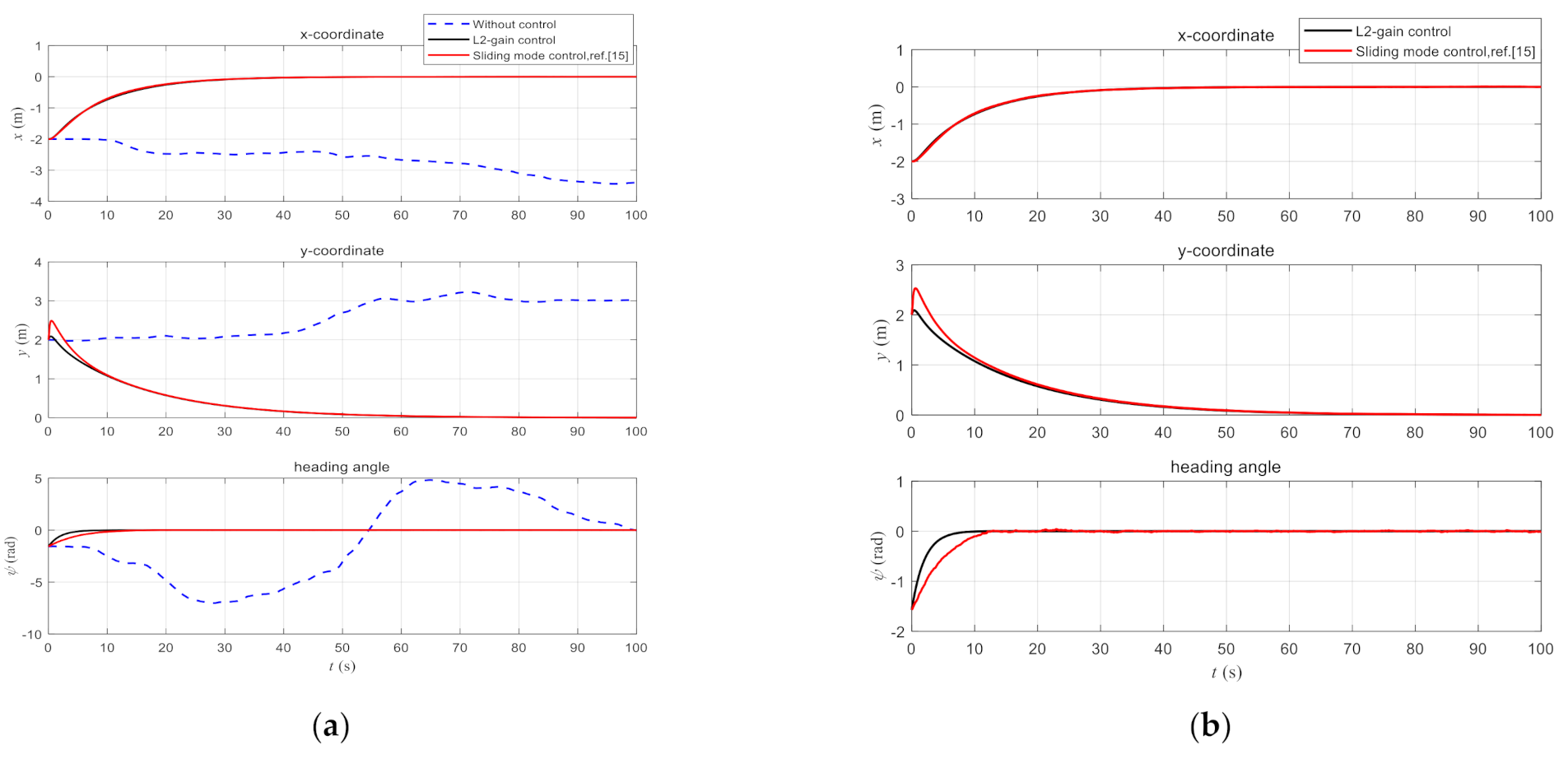
No asymptotic stability could be achieved but general stability instead. Nevertheless, errors could be made as small as possible by decreasing the L2-gain index γ₁, as illustrated in inequality (22).

(3)

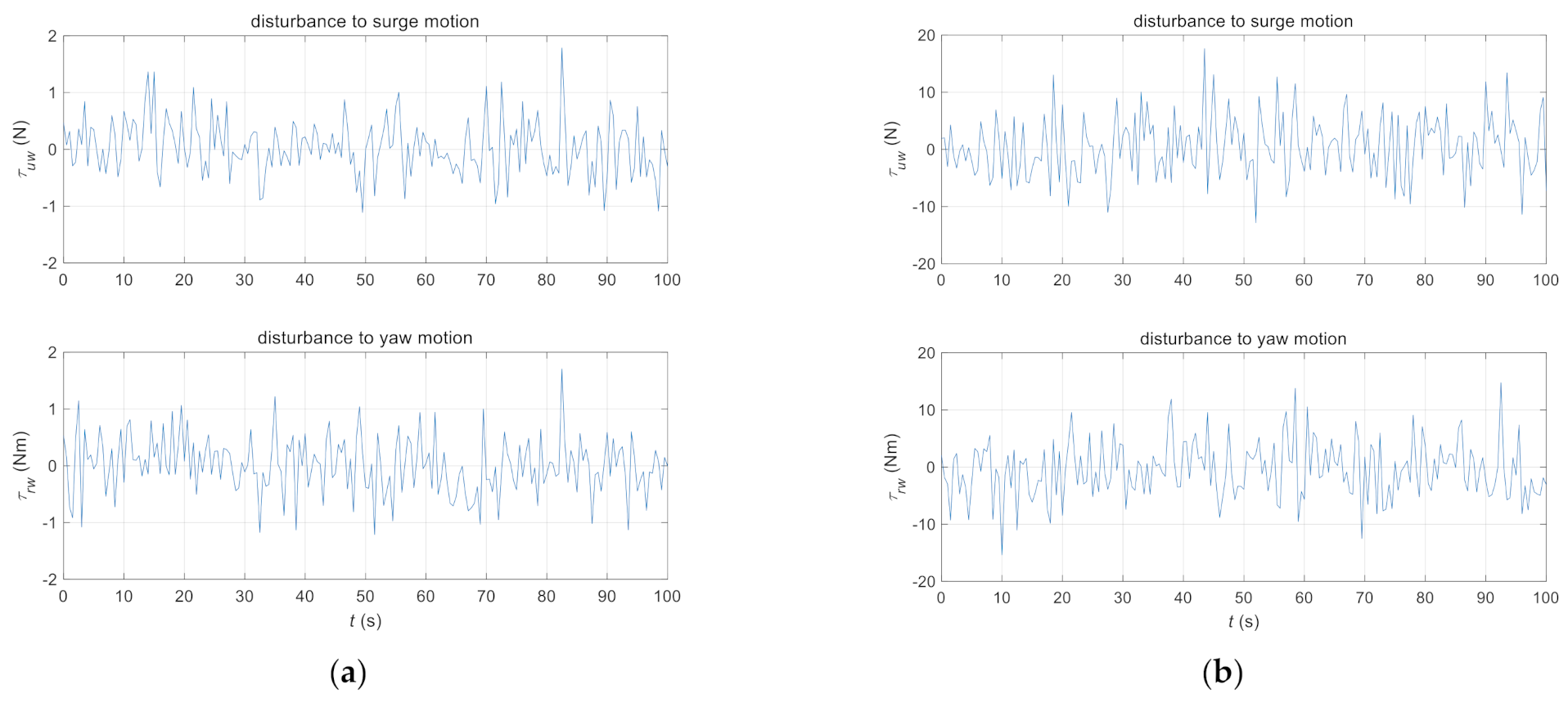
The disturbances considered in the study were uncertain and nonlinear in a real sense, which is consistent with the essence of environmental disturbances induced by wind, waves, and current. In many studies reported in literature, however, the disturbances were assumed as harmonic signals that could be estimated and compensated accurately in a close loop. There were difficulties with those estimation techniques when dealing with really uncertain signals.

In future work, efforts will be devoted to validating the proposed method using the experiment results. Efforts will also be devoted to the extension of this method to the other control issues of USVs, including path following, trajectory tracking, and docking/berthing.

References

1. Do, K.D.; Pan, J. Control of Ships and Underwater Vehicles: Design for Underactuated and Nonlinear Marine Systems; Springer Science & Business Media: London, UK, 2009. [Google Scholar]
2. Vu, M.T.; Choi, H.S.; Oh, J.Y.; Jeong, S.K. A study on automatic berthing control of an unmanned surface vehicle. J. Adv. Res. Ocean Eng. 2016, 2, 192–201. [Google Scholar] [CrossRef] [Green Version]
3. Brockett, R.W. Asymptotic stability and feedback stabilization. Differ. Geom. Control Theory 1983, 27, 181–191. [Google Scholar]
4. Pettersen, K.Y.; Egeland, O. Exponential stabilization of an underactuated surface vessel. In Proceedings of the 35th IEEE Conference on Decision and Control, Kobe, Japan, 13 December 1996; Volume 1, pp. 967–972. [Google Scholar]
5. Reyhanoglu, M. Exponential stabilization of an underactuated autonomous surface vessel. Automatica 1997, 33, 2249–2254. [Google Scholar] [CrossRef] [Green Version]
6. Laiou, M.C.; Astolfi, A. Discontinuous control of high-order generalized chained systems. Syst. Control Lett. 1999, 37, 309–322. [Google Scholar] [CrossRef]
7. Pettersen, K.Y.; Fossen, T.I. Underactuated dynamic positioning of a ship-experimental results. IEEE Trans. Control. Syst. Technol. 2000, 8, 856–863. [Google Scholar] [CrossRef] [Green Version]
8. Ghommam, J.; Mnif, F.; Benali, A.; Derbel, N. Asymptotic backstepping stabilization of an underactuated surface vessel. IEEE Trans. Control Syst. Technol. 2006, 14, 1150–1157. [Google Scholar] [CrossRef]
9. Ma, B. Global κ-exponential asymptotic stabilization of underactuated surface vessels. Syst. Control. Lett. 2009, 58, 194–201. [Google Scholar] [CrossRef]
10. Ghommam, J.; Mnif, F.; Derbel, N. Global stabilisation and tracking control of underactuated surface vessels. IET Control Theory Appl. 2010, 4, 71–88. [Google Scholar] [CrossRef]
11. Mazenc, F.; Pettersen, K.Y.; Nijmeijer, H. Global uniform asymptotic stabilization of an underactuated surface vessel. In Proceedings of the 41st IEEE Conference on Decision and Control, Las Vegas, NV, USA, 10–13 December 2002; Volume 1, pp. 510–515. [Google Scholar]
12. Tian, Y.P.; Li, S. Exponential stabilization of nonholonomic dynamic systems by smooth time-varying control. Automatica 2002, 38, 1139–1146. [Google Scholar] [CrossRef]
13. Dong, W.; Guo, Y. Global time-varying stabilization of underactuated surface vessel. IEEE Trans. Autom. Control 2005, 50, 859–864. [Google Scholar] [CrossRef]
14. Pettersen, K.Y.; Nijmeijer, H. Semi-global practical stabilization and disturbance adaptation for an underactuated ship. In Proceedings of the 39th IEEE Conference on Decision and Control (Cat. No. 00CH37187), Sydney, Australia, 12–15 December 2002; Volume 3, pp. 2144–2149. [Google Scholar]
15. Do, K.D. Practical control of underactuated ships. Ocean Eng. 2010, 37, 1111–1119. [Google Scholar] [CrossRef]
16. Ding, F.; Wu, J.; Wang, Y. Stabilization of an underactuated surface vessel based on adaptive sliding mode and backstepping control. Math. Probl. Eng. 2013, 2013, 324954. [Google Scholar] [CrossRef]
17. Zhang, Z.; Wu, Y. Further results on global stabilisation and tracking control for underactuated surface vessels with non-diagonal inertia and damping matrices. Int. J. Control 2015, 88, 1679–1692. [Google Scholar] [CrossRef]
18. Dai, S.L.; He, S.; Xu, Y. Transverse function approach to practical stabilisation of underactuated surface vessels with modelling uncertainties and unknown disturbances. IET Control Theory Appl. 2017, 11, 2573–2584. [Google Scholar] [CrossRef]
19. Lin, X.; Nie, J.; Jiao, Y.; Liang, K.; Li, H. Adaptive fuzzy output feedback stabilization control for the underactuated surface vessel. Appl. Ocean Res. 2018, 74, 40–48. [Google Scholar] [CrossRef]
20. Hinostroza, M.A.; Luo, W.; Soares, C.G. Robust fin control for ship roll stabilization based on L2-gain design. Ocean Eng. 2015, 94, 126–131. [Google Scholar] [CrossRef]
21. Songtao, Z.; Peng, Z. L2-Gain Based Adaptive Robust Heel/Roll Reduction Control Using Fin Stabilizer during Ship Turns. J. Mar. Sci. Eng. 2021, 9, 89. [Google Scholar] [CrossRef]
22. Luo, W.; Cong, H. Control for ship course-keeping using optimized support vector machines. Algorithms 2016, 9, 52. [Google Scholar] [CrossRef] [Green Version]
23. Vu, M.T.; Van, M.; Bui, D.H.P.; Do, Q.T.; Huynh, T.-T.; Lee, S.-D.; Choi, H.-S. Study on Dynamic Behavior of Unmanned Surface Vehicle-Linked Unmanned Underwater Vehicle System for Underwater Exploration. Sensors 2020, 20, 1329. [Google Scholar] [CrossRef] [PubMed] [Green Version]
24. Yu, R.T.; Zhu, Q.D.; Liu, Z.L.; Wang, Y. Decoupling implementation of global K-exponential stabilization of underactuated non-symmetric surface vessel. Control Decis. 2012, 27, 781–786. [Google Scholar]
25. Ishii, C.; Shen, T.; Qu, Z. Lyapunov recursive design of robust adaptive tracking control with L2-gain performance for electrically-driven robot manipulators. Int. J. Control 2001, 74, 811–828. [Google Scholar] [CrossRef]
26. Fossen, T.I. Guidance and Control of Ocean Vehicles; John Wiley & Sons: Chichester, UK, 1994; p. 331. [Google Scholar]
27. Fossen, T.I. Marine Control Systems: Guidance, Navigation and Control of Ships, Rigs and Underwater Vehicles; Marine Cybernetics: Trondheim, Norway, 2002; p. 447. [Google Scholar]
28. Zwierzewicz, Z. Robust and adaptive path-following control of an underactuated Ship. IEEE Access 2020, 8, 120198–120204. [Google Scholar] [CrossRef]
29. Tomera, M. Dynamic positioning system design for “Blue Lady”. Simulation tests. Pol. Marit. Res. 2012, 19, 57–65. [Google Scholar] [CrossRef] [Green Version]
Figure 1. Ship motion coordinate systems. (a) 6 Degree-of-freedom (DOF) ship motion, (b) 3DOF ship motion in the horizontal plane.
Jmse 09 00341 g001
Figure 2. Framework of control system for the underactuated surface ship with disturbances.
Jmse 09 00341 g002
Figure 3. Supply ship Far Scandia.
Jmse 09 00341 g003
Figure 4. Disturbance force and moment. (a) Disturbances at the level of 0.5*randn; (b) disturbances at the level of 5*randn.
Jmse 09 00341 g004
Figure 5. Position and orientation of the surface ship. (a) Disturbances at the level of 0.5*randn, (b) disturbances at the level of 0.5*randn.
Jmse 09 00341 g005
Figure 6. Velocities of the surface ship. (a) Disturbances at the level of 0.5*randn; (b) disturbances at the level of 5*randn.
Jmse 09 00341 g006
Figure 7. Trajectory of (x,y) of the surface ship under control. (a) Disturbances at the level of 0.5*randn; (b) disturbances at the level of 5*randn.
Jmse 09 00341 g007
Figure 8. Control forces and moments on the surface ship. (a) Disturbances at the level of 0.5*randn; (b) disturbances at the level of 5*randn.
Jmse 09 00341 g008
Figure 9. Training ship Blue Lady.
Jmse 09 00341 g009
Figure 10. Course-keeping control of the training ship Blue Lady. (a) Disturbances at the level of 0.05*randn (b) variation in heading angle and yaw rate (c) control forces and moments.
Jmse 09 00341 g010aJmse 09 00341 g010b