1. Introduction
The prediction of ship motion attitude is the prerequisite for ship maneuvering decision and motion planning. How to accurately construct a ship motion mathematical model to accurately predict the trend of ship motion has always been a popular research direction for vessels, semisubmersibles/submersible platforms, and unmanned underwater vehicles. Furthermore, due to the time delays and errors in obtaining ships’ dynamic data which will cause ship maneuvering errors and out-of-control drift, there are some great threats to the ships itself and shore-based facilities. Therefore, an accurate, rapid and economical ship maneuvering motion model is indispensable during sailing and berthing operations.
Compared with ship parametric modeling such as Abkowitz or MMG (Manoeuvring Mathematical Model Group) [
1], which is obtained through dynamics theoretical analysis after determining each parameter in the known model structure, non-parametric modeling [
2] is the response obtained directly or indirectly from the data analysis of the actual system, which avoids the problem of parameter drift of parametric modeling and the inaccuracy caused by the unmodeled dynamics. In addition, the construction of non-parametric modeling is also easier than parametric modeling. With the rapid development of machine learning and artificial intelligence, intelligent methods provide an effective way for non-parametric modeling, which has become popular in the ship motion modeling field from SVM (Support Vector Machines) [
2,
3] to ANN (Artificial neural networks) [
4,
5], from Bionic intelligence method [
6,
7] to deep learning [
8]. However, they are not invulnerable. For example, the optimal number of hidden layer neurons cannot be determined, and their generalization ability in ANN is limited. The size of training data is not easy to determine and model hyperparameters are not easy to grasp for SVM.
In ship motion identification modeling, LWL [
9,
10] is used as a non-parametric method [
11] like the above methods, to construct a non-parametric model of ship maneuvering motion. The difference of this method is that whenever it predicts a new sample value, it will solve the new parameter value according to the weight of the local model training set, so it can learn from a large amount of data and add data incrementally. And LWL can effectively overcome the problems of unmodeled dynamics and parameter drift [
12]. However, it does not provide a generative model for the actual system, and requires training data and test data to be independently generated in the same way. Moreover, the local model underlying architecture is in the least square form, i.e., a large effective data set is required to obtain a model with high accuracy, which seriously affects modeling efficiency. With the massive amount of information brought by big data, how to expand data-driven ship motion modeling is a question worth pondering in the LWL’s future development. The existing LWL algorithm for ship maneuvering motion modeling has tricky parameters that need to be adjusted [
7,
10] and these parameters strongly affect the deviation-variance and learning speed of the ship maneuvering motion mathematical model.
In order to overcome these issues, a method for LWL to identify ship maneuvering motion model based on Gaussian process (GP) [
13] is proposed. GP is also a non-parametric method. It combines the characteristics of the kernel method and Bayesian inference. It has the advantages of the above two machine learning methods and strict statistical theoretical basis. Meanwhile, the method is suitable for complex learning problems such as nonlinearity, small samples, and high dimensionality etc. and with strong generalization ability [
14]. Compared with ANN, SVM and other methods, it has the advantages of easy implementation, self-adapting hyperparameters, flexible non-parametric inference, and statistics significance of prediction results. On the other hand, the GP provides a generative model with black box automatic parameter adjustment. It has no significant requirements for the training data distribution of and has high learning capabilities.
Recently, GP has shown promising prospects in robot system modeling [
15,
16,
17], system identification [
18], time Series [
19] and ocean engineering applications [
20,
21] etc., which benefited from the continuous reduction of the computational complexity of the method. Simultaneously, its intuitive structure and Bayesian framework are very tolerant of sample data and hyperparameter. On the contrary, although the LWL can directly analyze the relationship between the input and output of the ship motion system [
9], this approach has high requirements on sample data and hyperparameter. Importantly, it is hard to make a compromise between modeling accuracy and computational efficiency [
11,
22]. The development of GP theory provides a favorable basis for rapid non-parametric modeling of ship maneuvering motion.
In this article, we propose Sparse Gaussian process based locally weighted learning (LSGP) for ship maneuvering motion non-parametric modeling. In this way, we retain the advantages of the two methods. Inspired by LWL, the training data is divided into local domains, and a GP is learned independently in the local domains during training and prediction. Using approximate reasoning technology, a sparse GP model is constructed in local domains without losing the advantages of LWL. The covariance matrix is solved by C++ on auxiliary platform to improve computational efficiency. Meanwhile, the generative model of LSGP can be better applied to engineering simulation.
The arrangement of this article is as follows.
Section 2 summarizes the background knowledge related to this content. The algorithm of LSGP is described in
Section 3. In
Section 4, an overview of the ship dynamics model, as well as ship identification scheme and simulation examples are given to verify the effectiveness of the proposed method.
Section 5 presents the main conclusions and further prospects.
2. Related Background Review of Non-Parametric Modeling Methods
The main content of this section is a background review of the non-parametric modeling knowledge required in this paper, which is about locally weighted learning and Gaussian Processes.
Generalized non-parametric modeling methods are about approximating a system (or function) through a number of n training points (or observations) . Here, x denotes the training input point and y the system output. We assume that the training outputs are corrupted by noise, , with , is a linear model usually. As shorthand notation, we merge all the training points into a training set and all corresponding output values into an output vector . Such that , with and , is the identity matrix, N and represents normal distribution.
2.1. Locally Weighted Learning
LWL uses the idea of locally learning to solve the task of compressing a large amount of data into a small number of local models. In the spirit of Taylor’s expansion, LWL’s idea is that simple models may be accurate in the local range, and it may be difficult to find good nonlinear features to capture the entire system globally, i.e., many good local models may constitute a good global model.
LWL trains
L local models, assuming that each local model has a local prediction in linear form
. When it works, the local predictions
are combined into a joint prediction at the query input
q as a normalized weighted sum. Hence, the prediction can be obtained according to Bayesian theory
with
with
is the weighted or attributed of the local model. The weight
determines whether data point
falls into the region of validity of local model
l, similar to a receptive field, and is usually characterized with a Gaussian kernel
where
h is the distance measure and
is the regression parameter. In the learning process, the shape of
h and the regression parameters of the local model
are adjusted by minimize the loss function between the predicted value and the observed target
The regression parameter
can be calculated incrementally using the least square method [
9,
11]. The distance measure
h determines the size and shape of each local model; it can be updated using cross-validation [
9], gradient method [
22], and intelligence methods [
7,
10].
An important observation is that Equation (
4) cannot be interpreted as least-squares estimation of the linear model
from Equation (
1). Thus, LWL cannot be converted probabilistically as one generative model for training and test simultaneously. Meanwhile, LWL requires several tuning hyperparameters, and its optimal value may be deeply dependent on the training data. Also, this high dependence makes this approach inefficient and time-consuming for learning and prediction. Here, we explored a probabilistic method to replace LWL. This method reduces the need for parameter adjustment and data requirements, but retains the characteristics of LWL.
2.2. Gaussian Process
A Gaussian process is a set of random variables, in which any finite-dimensional random variable obeys a uniform joint Gaussian distribution. It is a powerful alternative method for accurate function approximation in high-dimensional space.
The Gaussian likelihood can be obtained as
For the regression parameters
, suppose it is a Gaussian prior distribution with a mean value
of 0 and a covariance matrix of
, i.e.,
. The mean function is the a priori expectation of the unknown function. The covariance func-tion, or kernel, is typically selected by design as a measure of similarity between data points. Therefore, Combining the Gaussian prior distribution
and the likelihood function Equation (
5), the posterior distribution of the regression parameters can be calculated
The available mean and covariance matrix are
But the probabilistic interpretation of Equation (
6) has additional value over Equation (
4) of LWL because it is a generative model for all (training and prediction) data points, which can be used to learn hyperparameters conveniently.
Once we have the training data, we want to predict the function output
at a specific test input
. To accomplish this using GP method, the distribution of
can be predicted
Remark 1. Usually, by preprocessing the data, it is assumed that the prior distribution satisfies the mean equal to zero, here we use μ and to denote the prior distribution and and to denote the posterior distribution to distinguish them.
Notation 1. Definition , , , and so on, where is a non-linear function. Take them into Equation (8) we have So, we call the covariance function.
In the GP model, the covariance function
can measure similarity between system samples and determine the characteristics of the function
. The most commonly used covariance function is the Squared Exponential (SE) covariance function
Among them, l is called a relevance determination parameter, which measures the relevance of sample input and output. When has a strong dependence on x, l is smaller, and is more tortuous. When the dependence of and x is weak, l is larger, and is smoother. is the signal standard deviation of the covariance function, which adjusts the amplitude of . is the noise standard deviation, is the Kronecker symbol.
3. Approximation Algorithm for LSGP
For ship maneuvering motion modeling, this paper has constructed and modified LWL based on sparse GP to perform effective modeling, including sparsification, localization. These core tasks are described below.
3.1. Sparsification
The sparse Gaussian process reduces the computational complexity of regression (and optimization). Quiñonero-Candela et al. [
23] proposed the first unified framework to describe various methods at the time from the perspective of “approximate model, accurate inference” [
24,
25]. The framework of “approximate model, accurate inference” changes the assumptions made by the original model on sample data, and support points into the model in the form of parameters [
26]. Bui et al. [
27] also proposed a new unified framework, expounded from the perspective of “accurate model, approximate inference”. Under the new framework, the original model remains unchanged, and different approximate inference methods are used to reduce the time complexity. Using these methods, especially the FITC method [
28] that we will apply in this article, the runtime can be reduced to being linear with respect to
N, with only a limited reduction in how well the available data is being used, where
N is the number of training points.
The FITC method regards the ’Support points’ (or inducing points) as a virtual point, or a newly introduced parameter of the model, and optimizes the position of the induction point and other hyperparameters at the same time by means of parameter optimization. Suppose there are
M virtual sample points (not interfered by observation noise), called ’support points’, the input feature is
, and the corresponding function value
. Assuming that after these ’support points’ are given, the prediction points are independent of the training sample conditions, i.e.,
Under the condition of a given ’support point’, the training sample function values are conditionally independent, i.e.,
Approximate
of
can be calculated
where,
,
,
,
. For the ’support point’ set
M, we make it obey the Gaussian prior
So, we can get the marginal likelihood by Equations (
13) and (
14)
During training, the general method is maximizing the logarithmic marginal likelihood , the hyperparameter and the set of ’support points’ M are optimized through optimization algorithms.
When predicting through the GP model, first, we find the posterior distribution over ’support point’ using Equations (
14) and (
15)
where,
.
Given a new input
, the predicted distribution is obtained by integrating Equations (
14) and (
16)
The mean and covariance can be calculated as
where,
.
3.2. Localization
Based on the idea of local learning, the similarity between the query point
q and the local model is exploited to effectively cluster the system input data. Assumption: nearby query points may have similar target values. The local model is updated in a Gaussian process, as shown in
Figure 1.
In this study, the prediction of the system output
in local model
and their interpretation are carried out through an easy-to-interpret linear model, i.e., system output
for the
ith sample is assumed to be obtained using linear system in local model
where
is the system input in local model
l, the number
is determined by
w;
,
is a
D-dimensional weight vector for the
lth local model; and
is a Gaussian noise. Estimating
without any constraints is an ill-posed problem, we assume that functions determining
are generated from a multivariate GP. More specifically, the weight vector for the
ith sample for the
D-dimensional in
lth local model is obtained as follows
where,
is a Gaussian noise. Here, vector-valued function
that determines the regression parameters vector for each sample, and each element of
is generated from a univariate GP independently:
is the mean function, and is the covariance function.
Use the kernel function to learn local models, the similarity measure will be
, where
represents the distance between the query point
q and the training point
, and
h represents the hyperparameter, which is called the distance measure. It should be emphasized that in order to better perform local domain partitioning, any allowable kernel function can be used. Thus, the kernel can be varied in many ways. Here, the Gaussian kernel is used to cluster the local model
After sample data is partitioned, the kernel matrix is updated for each local model. The regression and prediction under these local models is the weighted average of the predicted mean of each local model for a query point. The optimization of the hyperparameters h of the kernel function is usually performed on sub-samples of the full training data. Here, Algorithm 1 gives the relevant process of the LSGP method.
| Algorithm 1 Localization and model learning of LSGP. |
- Input :
: iuput sample points; : output sample points; q: query points; : initial distance measure; : initial covariance parameter; M: initial support point set; - Output :
: generative model; , , : related parameters; - 1:
Calculate the distance d between the query point q and the sample point in the training set, such as Euclidean distance, Mahalanobis distance, etc.; - 2:
Use Equation ( 22) to cluster data to obtain the measure (or weight) of the local model corresponding to the query point q; - 3:
The training data sample points are weighted to construct a local domain centered on the query point q; - 4:
In the local domain, through Equations ( 10), ( 17), ( 18) obtain the covariance matrix and the Gaussian posterior in the Gaussian process, i.e., the construction of the local model; - 5:
Calculate the marginal likelihood by Equation ( 15), with logarithmic marginal likelihood as the loss function. Use the conjugate gradient to maximize the loss function to optimize the relevant parameters, , h, ; - 6:
Then, output the optimal relevant parameters, i.e., the distance measure of the local model , the support points , and the hyperparameters of the Gaussian process to obtain the optimal local model; - 7:
Obtain the generative model of ship maneuvering motion from optimal local model, and perform simulation prediction through the generative model.
|
Notation 2. When building a local model, calculating the Gaussian posterior and marginal likeli-hood of the model requires the calculation of the covariance matrix and its inverse. For the ship motion system, it is easy to produce singular data when performing steady manoeuvring. Therefore, LU-decomposition is used to process the covariance matrix to reduce calculation errors. For solving the inverse covariance matrix, Cholesky-decomposition can be used, i.e., cholesky , to improve calculation efficiency.
4. LSGP for Identifying the Ship Maneuvering Motion System Model
In this section, the relevant content of ship motion identification modeling based on the LSGP method is explained, and secondly, explanatory learning examples will be provided to verify the performance of the proposed scheme. In order to achieve this goal, taking the plane motion model of the ‘Mariner’ class vessel as the research object. In addition, two LWL modeling schemes are proposed, including Global LWL [
9] and Local LWL [
22] for comparison. These simulations are all carried out on a computer with 3.2 GHz CPU and 8 GB RAM.
4.1. Ship Dynamics Overview of Ship Maneuvering Motion
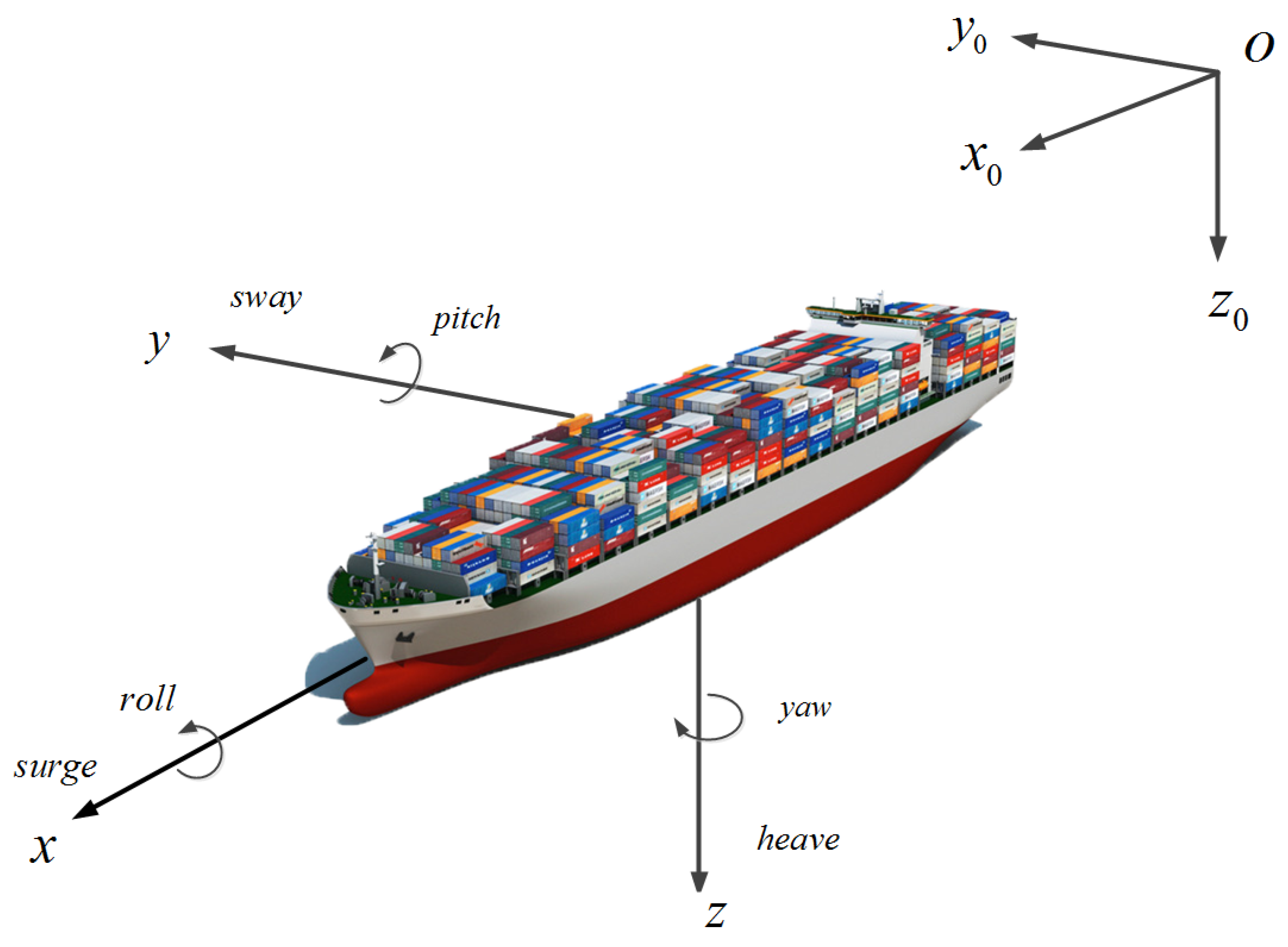
Ships sailing at sea can be approximately regarded as a rigid body. In order to better describe the ship’s motion state, a space-fixed coordinate system
and a body-fixed coordinate system
are introduced, as shown in
Figure 2. It can be seen that the actual motion of a ship is very complex, and it has 6-DOF generally. For most ship motions and their control problems, heave motion, pitch motion and roll motion can be neglected, only surge motion, sway motion and yaw motion can be discussed, which can satisfy enough engineering requirements. Therefore, simplifies the ship motion into a 3-DOF plane motion. At the same time, in the ship coordinate system it is more simple and straightforward to study the movement of the ship in the surrounding flow field and the interaction between fluid and hull.
According to the characteristics of the ship’s motion and the effects of the forces on the hull, the forces acting on the ship can be divided into three categories [
29]: (1) the main power
, the force generated by the ship’s power system, including the propeller thrust and the rudder force. (2) Environmental interference force
, i.e., the force acting on the ship by external factors such as wind, waves and current. (3) Hydrodynamic force
, i.e., the movement of the ship in the fluid under the action of the main power and the environmental inference force, and the reaction force generated by the fluid on the movement of the ship, including the fluid inertial force and the fluid viscous force etc. Therefore, the composition of the force and moment of the ship can be expressed as
According to the rigid body momentum theorem, the momentum theorem of rigid body centroid motion and Newton’s law of motion, ship motion can be expressed as follows
where,
m is the mass of ship;
is the longitudinal coordinate of the ship gravity center;
is the yaw moment of inertia about
z axis;
,
and
denote the surge acceleration, sway acceleration and yaw angular acceleration corresponds to
u the surge velocity,
v the sway velocity,
r the yaw angular velocity;
,
and
is the projection of the total forces and moments
F,
M in different directions.
Generally, in the study of ship motion, the motion law of ship’s gravity center is mainly considered. Therefore, the origin of the body-fixed coordinate system can be taken at the center of gravity, i.e.,
. In addition, the forces and moments in ship motion are related to the characteristics of the ship motion (velocity, acceleration etc.), the hull characteristics and the maneuvering factors (rudder angle
, propeller speed
n, etc.). The Equation (
24) can be written as follows
The main task of identification modeling is to find a suitable and accurate , and to better describe the ship maneuvering motion system.
4.2. System Identification Modeling Experiment
Although it is also possible to use the strategy of directly considering the relationship between ship’s motion states [
2,
5,
9,
10] in non-parametric identification modeling (i.e., to study the relationship between ship motion
,
,
at
kth time and
,
,
at
th time), here, we adopt a strategy that considers the relationship between the ship’s motion states and the ship’s external forces, (i.e., we care about the relationship between the ship’s motion
,
,
at
kth time and
,
,
, at
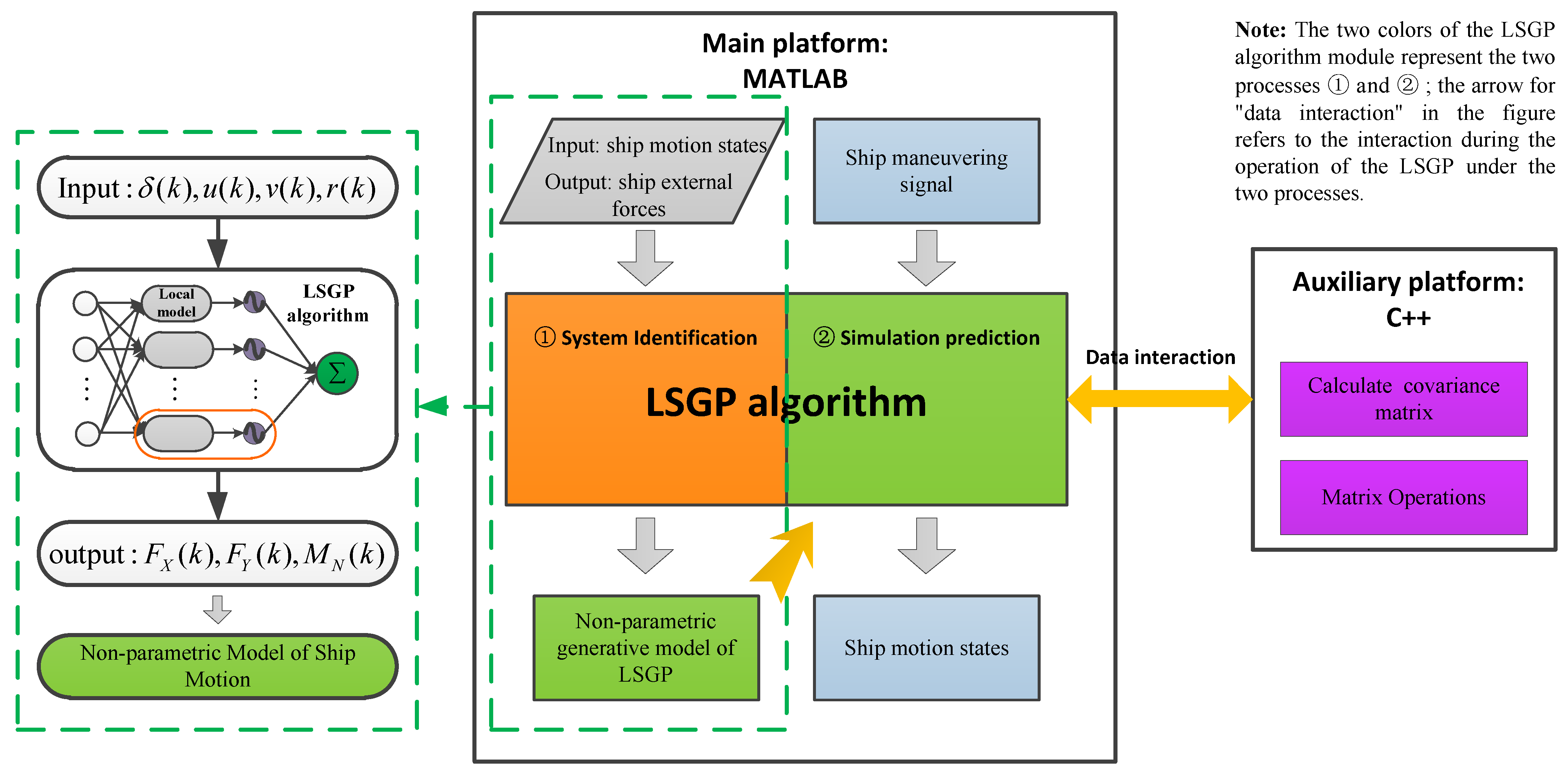
kth time) as shown in
Figure 3, the relevant content in the green dashed box. This way, getting rid of the discrete processing mode of the ship motion system in the time domain is a continuous-time system mode. At the same time, during model training and simulation prediction, the LSGP-based modeling method has matrix operations, so in addition to the LU-decomposition and Cholesky-decomposition processing of the matrix mentioned in the third section above, the correlation matrix operations are transplanted to the C++ language Environment, as shown in
Figure 3, to improve computing efficiency.
Data is the first element of recognition, and the quality of the data will directly affect the recognition result. For the LWL method, it is extremely important for data collection and processing. Therefore, in references [
5,
9,
10], several ship maneuvering tests (8-shaped test, sinusoidal signal) are designed and processed for this purpose to make the collected data as much as possible. Information, most of the design tests are more complicated and are not suitable for actual ship maneuvering. Here, we only use the zigzag test (see
Table 1) mentioned in the IMO MSC.137 (76) and ITTC Guidelines (2017) for data collection and model identification learning.
The well-known ’Mariner’ class vessel is taken to establish the experimental maneuvering motion model [
2,
9]. Simulation of
/
zigzag test, which is conducted with initial sailing speed of 15 knots (7.72 m/s), sampling time is 700 s and the interval is 1 s, i.e., 700 measurement pairs of
u,
v,
r,
, as the training set for identification of ship hydrodynamic model. In this paper, the propeller rotation change is not considered. The rudder angle is the system input regarded as the system excitation. Therefore, the rudder angle is a known variable. In order to verify the generalization and prediction capabilities of the proposed LSGP-based ship motion model, we considered a convincing maneuvering test as the inspection plan. For the sake of simplicity, the design speed
= 7.2 m/s (15 knots) is the initial speed, and two typical zigzag maneuvers expressed by ‘ZZ-
(heading angle)-
(rudder angle)’, namely ZZ-
-
and ZZ-
-
; use turning test ‘T-
(rudder angle)’ to verify the ship’s turning test performance, and give experiments on T-
; at the same time, the simulation experiments and the reference model were compared. The simulation experiment situation is shown in
Table 1. It is pointed out here that the ‘reference model’ used in the article is based on the parameter model obtained through the PMM test, and the parameters and architecture of the reference model can be found in [
2,
29].
The initial parameter values about LSGP are generated randomly during training ship motion model, where, , , The ’support point’ is a random sample of in the training set, the training step is set to 1000. The marginal likelihood is maximized by conjugate gradient to learn the best generative model and parameters.
4.3. Simulation Results and Analysis
In order to better explain the pros and cons of the LSGP algorithm, we demonstrate how the proposed algorithm can be executed on full-scale experimental data for different manipulation scenarios. The proposed ship motion model based on LSGP can better approximate the original ship model. As shown in
Figure 3, since the corresponding system input and output are different from the previous identification modeling, the relationship between the ship’s motion state and the external force on the ship is considered.
Figure 4,
Figure 5 and
Figure 6 shows the results of three sets of simulation experiments in
Table 1. It can be seen that the non-parametric model under LSGP method has good generalization, except for deviation of the Yaw moment N of the simulation prediction. This is because the ship Yaw moment is relatively complex, has strong nonlinearity and is difficult to decouple from the motion state in other DOF.
In the zigzag test, the nonlinearity of the ship motion state is more serious. The learning error of LSGP in
Figure 4 and
Figure 5 is mainly manifested in the Yaw moment. This is because the Yaw moment is more complicated than other DOF, and its value is not in the same order of magnitude as other degrees of freedom. The prediction of the ship’s turning test shows good performance in
Figure 6, which avoids the divergence due to the singular value generated when the data is close to zero by the ship’s steady motion.
Notation 3. Due to the large magnitude difference between the various physical quantities of ship motion, which are easily affected by ship size, speed, fluid physical parameters, etc., they have been processed in a dimensionless manner. The various physical quantities in Figure 4, Figure 5 and Figure 6 are in dimensionless form. From the above simulation results that the LSGP algorithm has a certain prediction simulation effects, and low requirements for training data. This property is determined by the nature of the LSGP algorithm. It is the main line of this paper to predict the external force of the ship through identification modeling, and to further calculate the trend of the ship’s motion at the next moment according to the Equation (
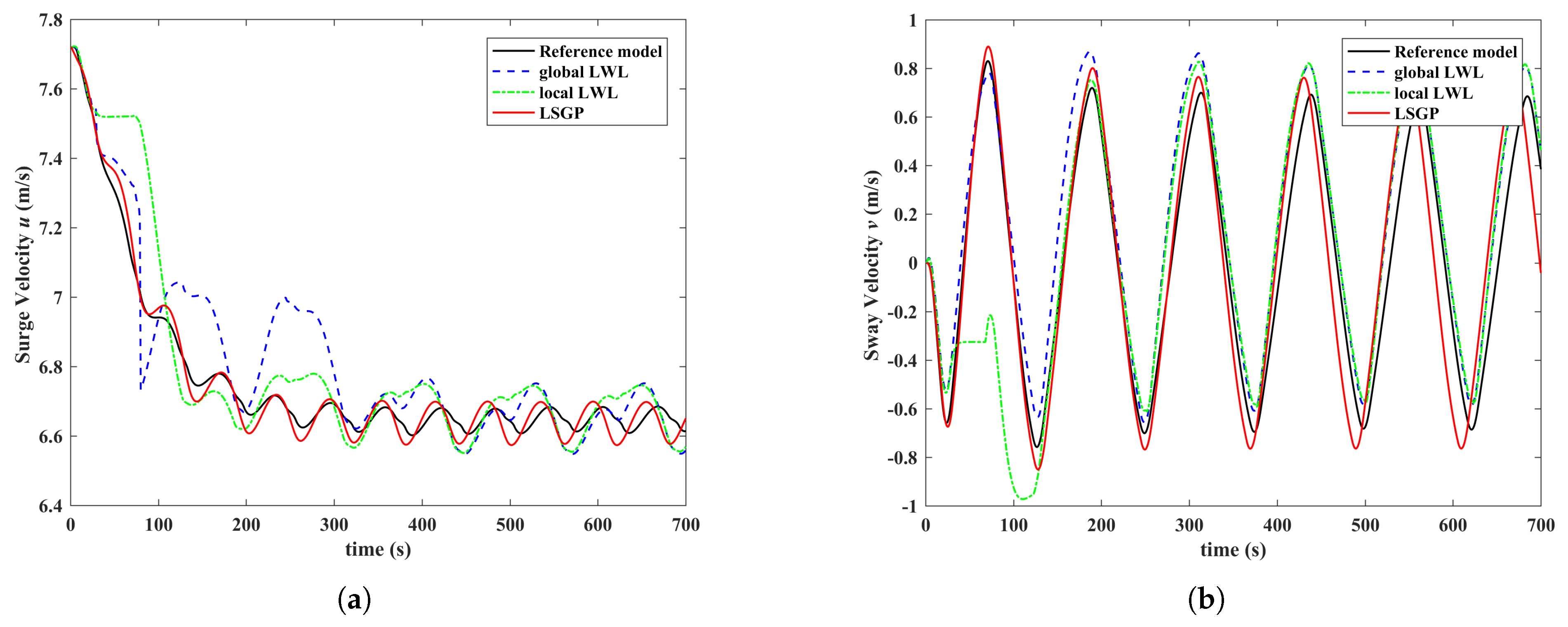
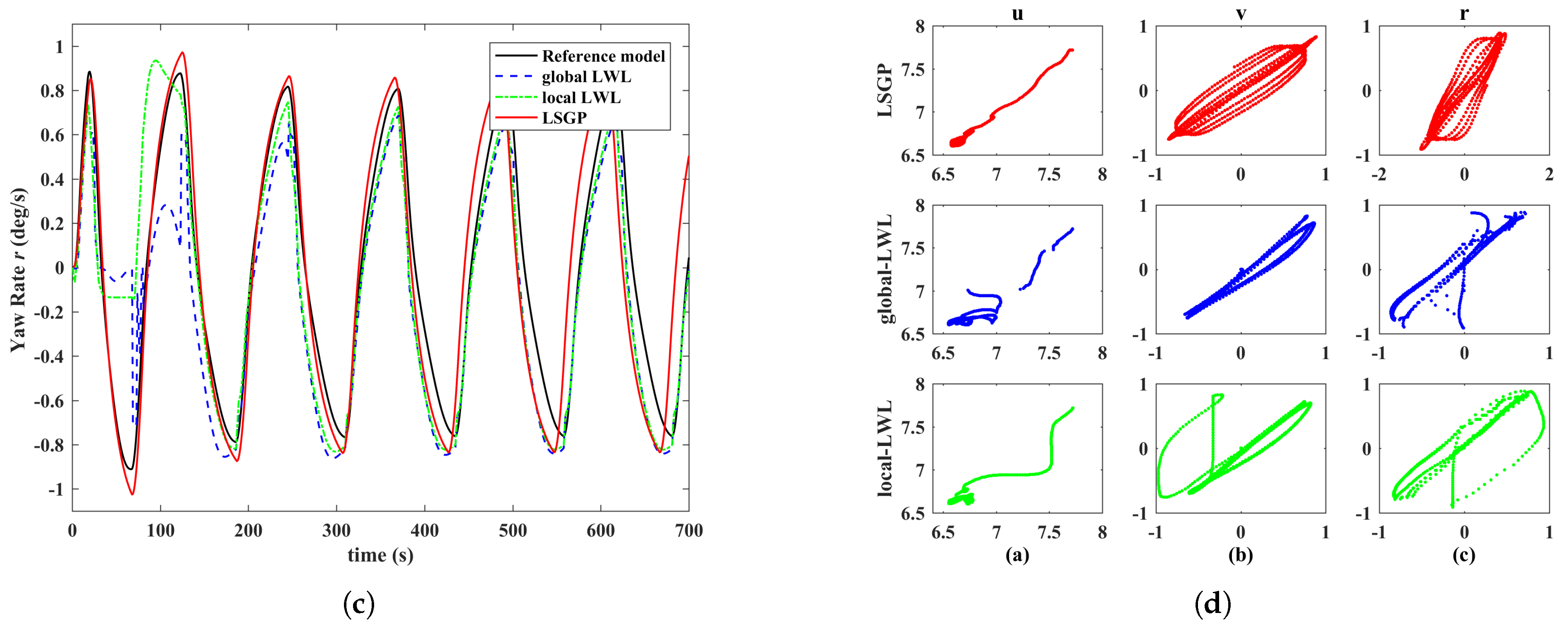
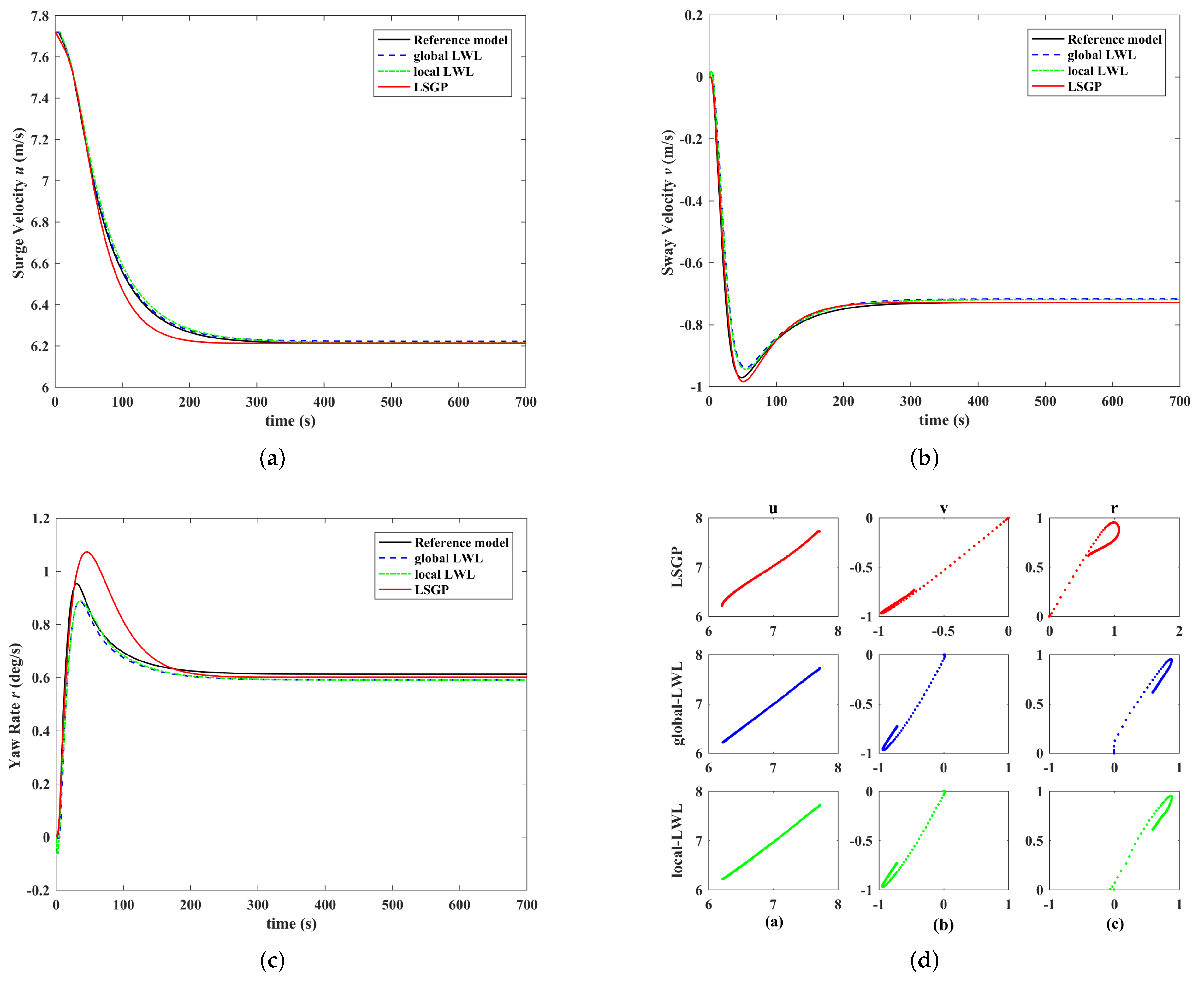
25) in real time, and then to predict the state and trajectory of the ship’s motion. The simulation prediction results of the mariner test are shown in
Figure 7,
Figure 8 and
Figure 9, and a comparison based on the two LWL (global LWL [
9], local LWL [
22]) algorithms is also given.
As can be seen from
Figure 7, the simulation of LWL does not work effectively. Compared to the Gaussian process, LWL cannot effectively build a generative model. For tests like ZZ-
-
, it is not included in the features of the LWL training set, so simulation predictions cannot be made well. It directly shows that LWL has high requirements for training data and is not easy to use in applications. On the contrary, LSGP has good generalization ability. In order to quantitatively describe the differences between different methods, the following
Table 2 gives mean squared error (MSE) evaluation criteria for comparison
where,
represents the reference model,
represents the simulation prediction, and
n represents the data length.
It can be seen intuitively from
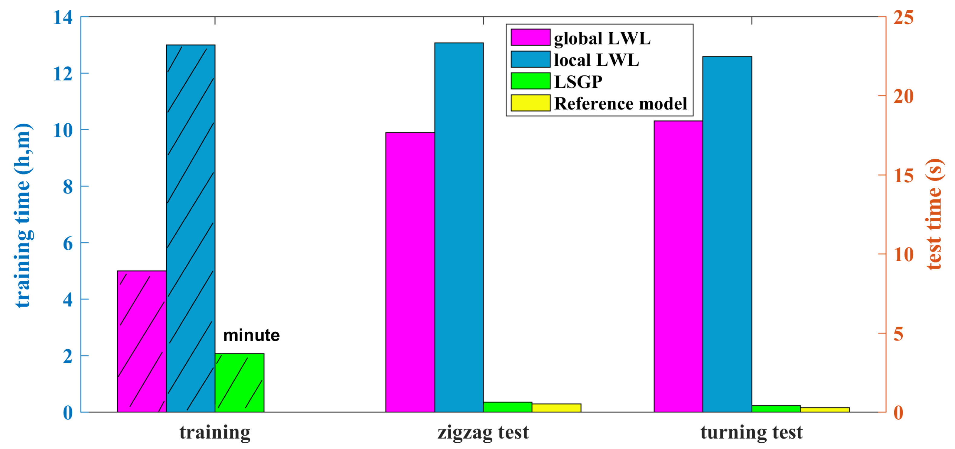
Table 2 that LSGP has advantages over other methods in the zigzag test, generally, Global LWL < local LWL < LSGP, and the simulation accuracy in the turning test needs to be improved, which is related to the fact that our training data does not include turning data. At the same time, three algorithms are given about the time spent in training and simulation prediction, as shown in
Figure 10.
There are two methods for the GP to calculate the inverse matrix, one is to directly use the traditional Gaussian elimination method, and the other is matrix decomposition. When the dimension of the matrix is too large, the inverse calculation of the matrix by Gaussian elimination method needs to be calculated in blocks. On the other hand, for the ill-conditioned matrix generated in the ship steady motion, coupled with the influence of the computer truncation error, the direct calculation using the Gaussian elimination method cannot obtain accurate results, and the time complexity is . We use Cholesky decomposition, i.e., , its time complexity is .Usually the dimension of input space is limited, so the transition matrix is defined on the auxiliary platform to store the distance between input data, that is, the elements of the covariance matrix: . represents the kth dimension element of the ith dimension input of the data. These matrices can be used to reduce the calculation amount, its time complexity is .
The time spent on training and simulation prediction for the LSGP algorithm decreases exponentially in
Figure 10. In training part, LSGP is reduced by 100 times compared with Local LWL, and it is also reduced by 10 times in simulation prediction. At the same time,
Table 3 gives different training data method requirements, among them, LSGP has very low requirements for training data. It only needs a set of zigzag tests as training data, which is also easy in engineering practice. For the’reference model’ based on mechanism modeling, LSGP can make the computational time consistent with the reference model while ensuring the modeling accuracy. This advantage is self-evident. On the one hand, LSGP is a data-driven model, which can provide considerable results based on limited data without the need to use physical tests, empirical formulas and CFD methods to determine model parameters, thus reducing operational difficulty and economic investment. On the other hand, non-parametric modeling can avoid the parameter drift, which is not limited by the model structure. It is a feasible method when the ship principal particulars are not easy to obtain. At the same time, decreasing the calculation time of non-parametric modeling to be consistent with that of the reference model can provide preparations for future online identification modeling.
5. Conclusions and Prospects
This paper introduces the development of a new local weighting scheme based on sparse Gaussian process, which is used for ship maneuvering identification modeling in a full-scale ocean environment. The main advantages of this scheme are low requirements for training data, high computational efficiency, and no need to know the structure of the ship maneuvering model, which is easy for engineering practice. As far as the author knows, the existing research work rarely considers the choice of model structure, which is meaningful and inevitable in actual ship engineering. Application experiments show the engineering practicability, effectiveness and generalization of the scheme. In addition, the program can also be extended to other online identification or prediction systems in the field of ocean engineering.
Further work will focus on ship maneuvering identification modeling under the dual-rate measurement engineering environment considering the speed of the ship’s main engine, and the influence of factors such as wind and waves should also be considered. At the same time, the ship maneuvering motion modeling method based on the LSGP is not perfect and limited to the Gaussian noise distribution assumption. So, the next step is to consider breaking the Gaussian noise distribution assumption and considering the influence of time factors, as well as to research the relationship between localization and sparseness in LSGP to improve ship motion modeling accuracy as much as possible.

