An Integrated Dynamic Model and Optimized Fuzzy Controller for Path Tracking of Deep-Sea Mining Vehicle

Abstract

The capability of path tracking largely determines the operational efficiency of deep-sea mining vehicles. In this paper, the relationships of vehicle–sediment mechanical interaction were obtained by sinkage and shear tests. Then, an overset grid method was used to establish the computational fluid dynamics (CFD) model of the vehicle, and the spatial hydrodynamic distribution was calculated in different motion states. Based on the above research, a multi-body dynamic (MBD) model of the mining vehicle was developed, which considered the spatial hydrodynamic effects and the mechanical interaction between vehicle and sediment. In addition, a path-tracking controller based on fuzzy logic control was proposed. A genetic algorithm optimized the fuzzy rules through co-simulation between the controller and the MBD model. Finally, the co-simulation results of the vehicle which moved along the expected path indicated that the performance of the optimized fuzzy controller was preferable to the original fuzzy controller.

1. Introduction

With the constant decrease of mineral resources on land, many countries and organizations are attracted to the rich mineral resources contained in the seafloor. At present, the promising commercial marine mining system is the type of hydraulic lifting pipeline, including a marine mining vehicle as a core component [1]. The potential market of deep sea mining vehicle is large. Due to the influence of complicated hydrodynamic effects and particular mechanical interaction between vehicle and sediment, it is difficult to attain satisfactory path-tracking performance for the mining vehicle.

Before exploration of the path-tracking control strategy of deep-sea mining vehicles, a dynamic model is needed. Hong et al. [2] conducted dynamic simulations of a tracked vehicle through a simplified dynamic model and investigated steering performance. Kim et al. [3,4] compared the advantages and disadvantages of two model types on tracked vehicles and used a large number of numerical simulations to analyze the hydrodynamic effects. For a seafloor-tracked vehicle, a single-body model was conducted to achieve a fast analysis of the moving process [5]. The above dynamic model greatly simplified the actual situation to facilitate the numerical calculation. In a vertical plane, the forces and moments that validated the Reynolds Average Navier–Stokes equations were measured for an autonomous underwater vehicle (AUV) [6]. Phillips et al. [7] utilized an analysis of CFD to predict hydrodynamic forces and moments for its accurate prediction. The hydrodynamic damping was acquired by the computational fluid dynamic approach in an open-frame remotely operated vehicle (ROV) [8]. The CFD method has more accuracy than the empirical formula for the calculation of hydrodynamic effects. For an underwater tracked vehicle with a ladder trencher and a rock-crushing tool, the influence between the mining tool part and the tracked vehicle part was studied for optimized design of the underwater track vehicle system [9,10]. Li et al. [11] studied a single track shoe to improve the tractive performance and optimize the structural parameters of the track. For a saturated soft-plastic soil, Wang et al. [12] proposed a shear stress-displacement empirical model validated by a track segment shear test. Baek et al. [13] studied the mechanical properties of the soil thrust by the limit equilibrium analysis technique on clayey soil. Owing to the particular environment of the seafloor, the research studies of deep-sea soil are essential. Vu et al. [14] utilized a number of numerical simulations of an underwater construction robot in up-cutting mode to analyze the change of forces, moments, energy, and power in different conditions. For an AUV, Sun et al. [15] built a dynamic model to study the performance of path tracking. Dai et al. [16,17] extended a new simulation to obtain relationships of the seabed sediment by the discrete element method and used the Reynolds stress model to complete CFD simulation. Many researchers have done outstanding work in the field of underwater dynamics modeling, but most of them have conducted deep research in local areas such as rapid modeling, hydrodynamic effects, and deep-sea soil mechanics. Few people combine the above achievements to establish a more comprehensive dynamic model. However, a dynamic model that fully considers the influence of various factors is essential in the study of path tracking for deep-sea mining vehicles.

For an excellent accuracy of path tracking, a suitable control strategy is essential. Yeu et al. [18] constructed a vector pursuit algorithm for the generation of a specified motion path and proposed a new control method through traction force and track slip; this control strategy was effective but also complex. Hong et al. [19] formulated an algorithm that contained the control of forwarding velocity and heading angle for the path tracking of a tracked vehicle; this control scheme was widely accepted. Zhang et al. [20] investigated a hybrid fuzzy PID controller for an ROV and used the small gain theorem to analyze the stability. Londhe et al. [21] proposed the robust nonlinear PID-like fuzzy controller for trajectory tracking and validated its better and robust control performance. Lamraoui and Qidan [22] proposed two path-following controllers based on active disturbances rejecter control to obtain a high tracking accuracy. The fuzzy logic control was widely applied in path tracking for its outstanding performance in nonlinear systems. Based on a particle swarm optimization algorithm, a fuzzy logic controller was designed to control the ROV vertical trajectory [23]. For a dynamic positioning system of vessels, an adaptive fuzzy controller was developed to eliminate the influence of environmental disturbances and develop the control accuracy [24]. Chen et al. [25] developed the fuzzy controller for path tracking and heading tracking of an ROV, which was optimized by a genetic algorithm. Londhe and Patre [26] proposed an adaptive fuzzy sliding mode control scheme for an AUV and eliminated the problem of chattering. Dai et al. [17,27] researched an adaptive neural-fuzzy control strategy and validated its better performance with collaborative simulations, and they proposed a fuzzy adaptive PID algorithm as the motion control strategy for an underwater operating vehicle. Based on the superiority of fuzzy control, many scholars have conducted in-depth research on the optimization methods of fuzzy controllers, which mainly focus on the optimization of fuzzy rules and affiliation functions. It is valuable to use genetic algorithms to optimize fuzzy controllers to achieve more accurate trajectory tracking of deep-sea mining vehicles.

From the previous research, it can be found that the establishment of the dynamic model of a deep-sea mining vehicle was seldom considered with the spatial hydrodynamic effects and mechanical interaction between vehicle and sediment. Simultaneously, the rules of fuzzy control are easily affected by the experience limitations of the designer, which may lead to reduce control performance. So, in this paper, a multi-body dynamic (MBD) model of a deep-sea mining vehicle, which considers the mechanical interaction between vehicle and sediment and spatial hydrodynamic effects, was developed first. Next, a fuzzy controller that contained double input and output was proposed for path tracking, and a genetic algorithm optimized the controller through the collaborative motion simulation. Finally, the performance of the optimized fuzzy controller was analyzed.

2. Establishment of the MBD Model

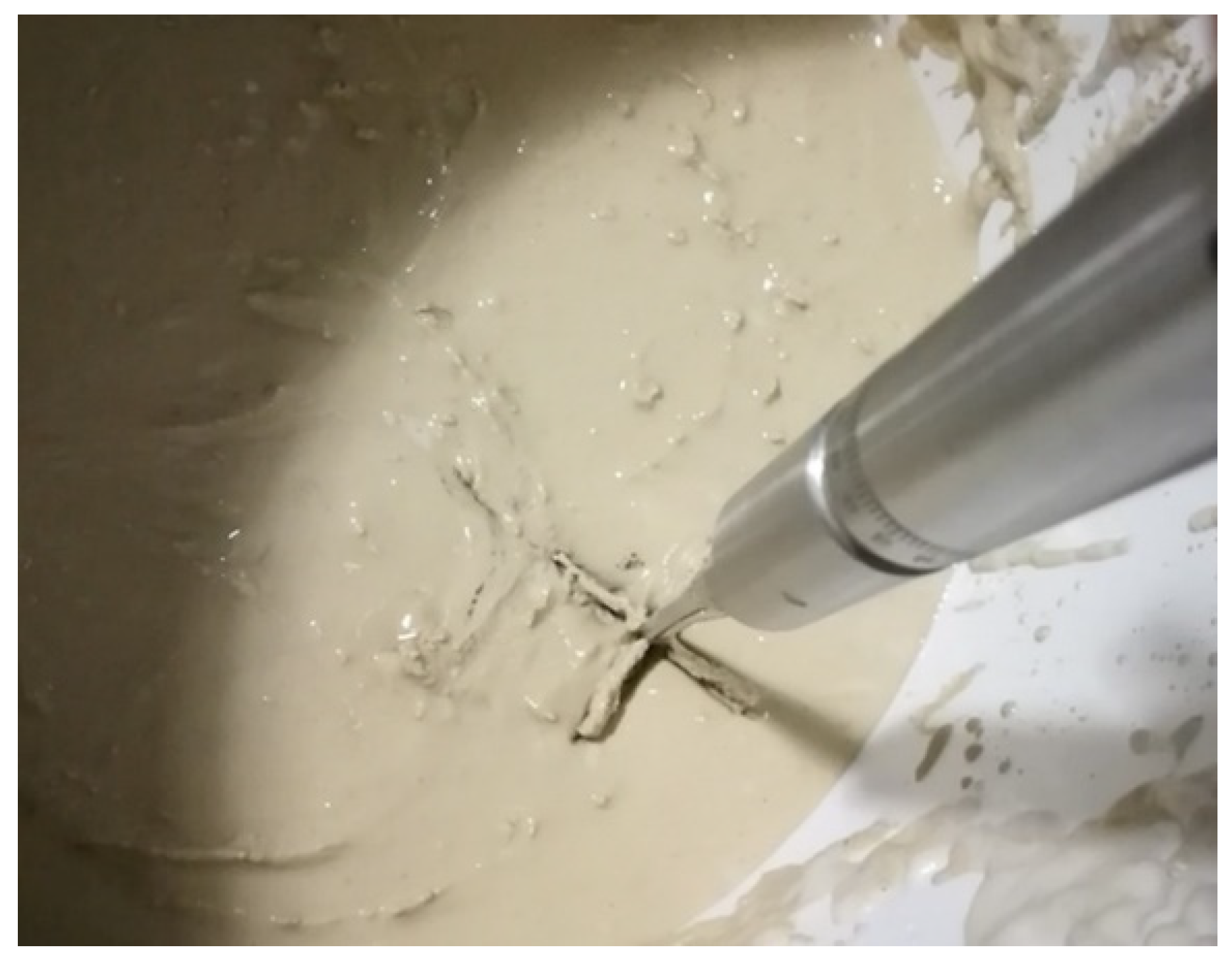
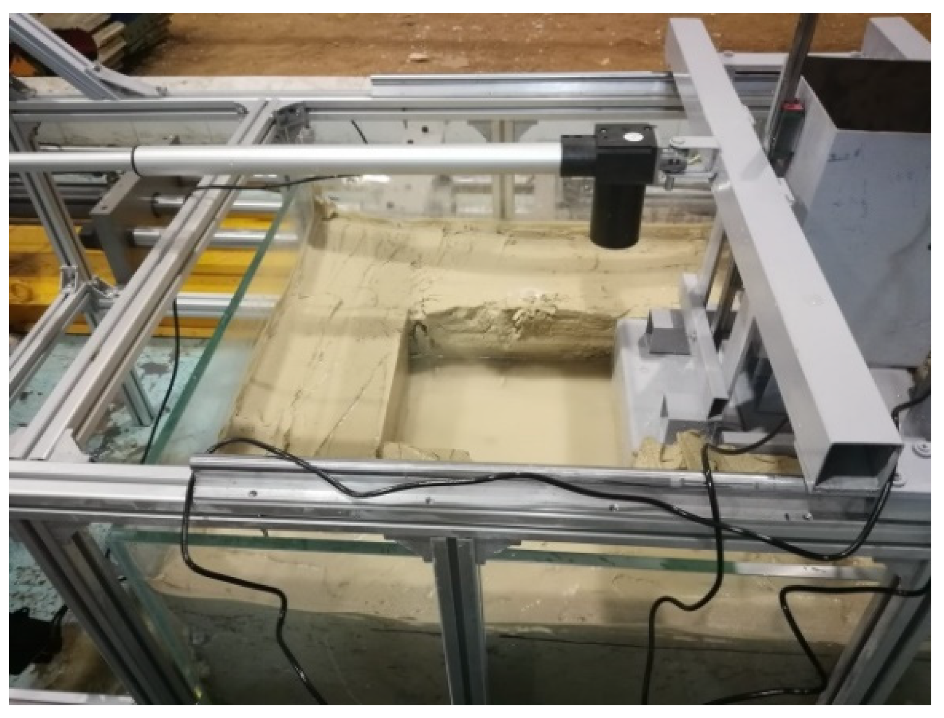
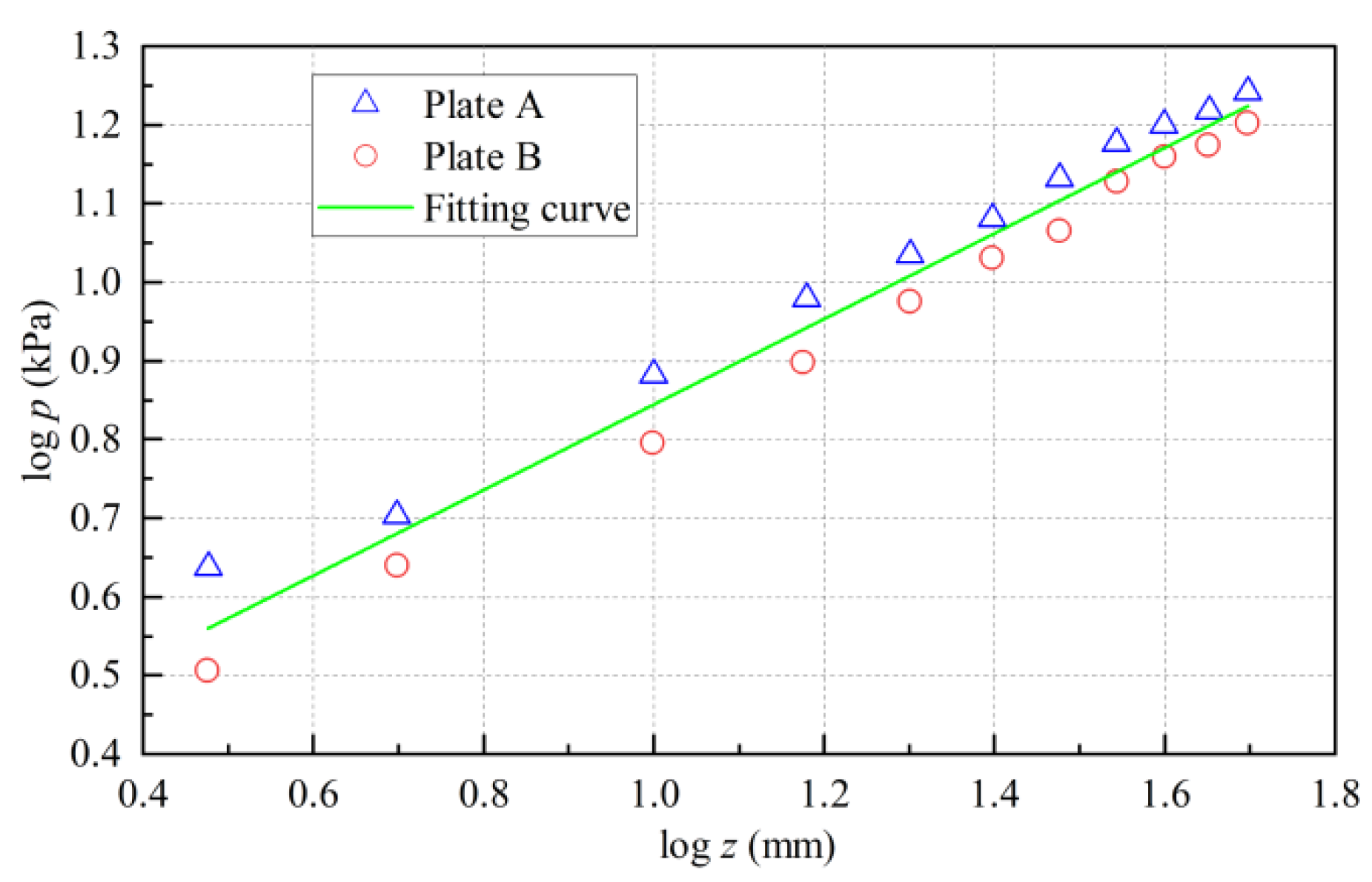
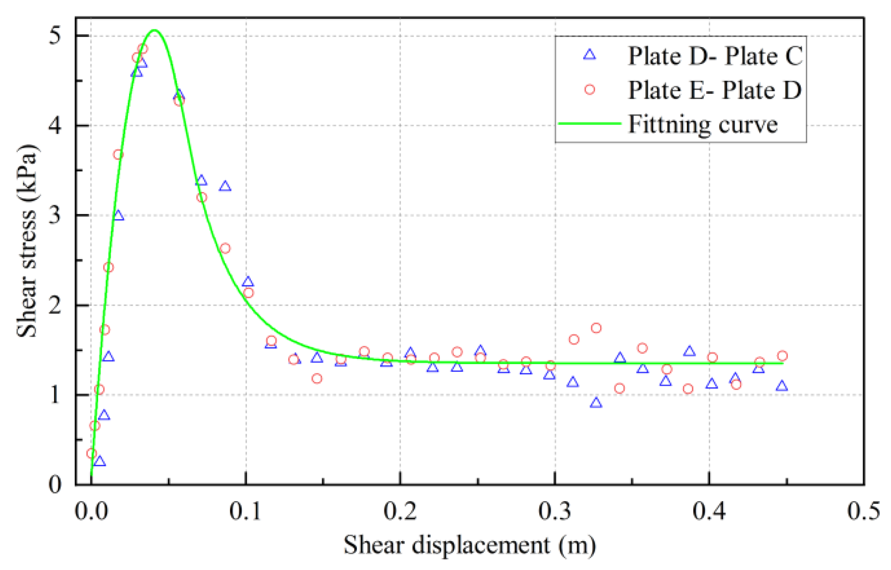
2.1. Vehicle–Sediment Mechanical Interaction

On account of the particular environment of the seafloor, seabed sediment properties are utterly different from terrestrial soil, so it is necessary to conduct special research on vehicle–sediment mechanical interaction when the deep-sea mining vehicle is modeled. The mechanical interaction between the vehicle and sediment is mainly manifested in the pressure–sinkage characteristic and shear stress displacement.

It is hard to measure the mechanical properties of the interaction between the vehicle and sediment by in situ tests, so laboratory simulation is considered for this study. The substrate at the surface layer of 15–20 cm is used as the bearing layer and shear traction layer when the mining vehicle travels on the seabed, so the physical force characteristics of the substrate at this layer are used as the basis for formulating the simulated substrate. As shown in Figure 1, the simulated sediment is mixed with bentonite and water and tested by a cross plate shear tester. Its mechanical properties displayed in

Table 1. Comparison between in situ test data and simulated sediment test data.

Data Type	In Situ Test Data	Simulated Sediment Test Data
Shear strength (kPa)	4–6.5	4.9
Average moisture content (%)	90–130	110
Wet density (g·cm−3)	1.2–1.5	1.3
Dry density (g·cm−3)	0.54–0.65	0.62
Porosity ratio	3.11–4.13	3.28

were highly consistent with the in situ test data.

The pressure–sinkage characteristic expresses the ability of the soil to resist deformation under the normal load. Bekker [28] conducted a number of experiments and proposed the following formula for the pressure–sinkage property of homogeneous soil:

$$p=\frac{1}{2}\left(\frac{k_c}{b}+k_{\phi }\right)z^n$$

(1)

where $p$ is the normal pressure; $k_c$ is the soil cohesive; $k_{\phi }$ is the friction modulus; $b$ is the width of the plate; $z$ is the sinkage; $n$ is the soil deformation exponent.

The characteristic of brittle soil displays a hump of maximum shear stress. The equation that describes the relationship between shear stress and displacement of the brittle soil is proposed by Wong and Preston-Thomas [29], and it was given by:

$$\tau =(c+p\tan \phi )k_r\left\{1+\left[\frac{1}{k_r\left(1-e^{-1}\right)}-1\right]e^{1-j/k_{\omega }}\right\}\left(1-e^{-j/k_{\omega }}\right)$$

(2)

where $c$ is the cohesive, $\phi$ is the internal shearing resistance, $k_r$ is the ratio of the residual shear stress to the maximum shear stress, $j$ is the shear displacement, and $k_{\omega }$ is the shear deformation modulus.

During the sinkage test, the simulated flat plates of different sizes were pressed perpendicularly into the simulated sediment. The size of simulated plate A is 375 mm long and 150 mm wide, and plate B is 240 mm long and 120 mm wide. To effectively remove the effect of soil pushing resistance during the horizontal movement of the shear displacement test, three simulated track plates named plate C, D, and E in Figure 2 were designed as the same width and height. However, their lengths were 150, 300, and 450 mm, respectively. The pushing resistance could be eliminated by subtracting the measured data from each track plate. The sinkage test data of plates with different sizes and the fitting curve of the average value were demonstrated in Figure 3. In different size plates, the changing trends of the compressive pressure–sinkage relationships are relatively consistent. Equation (2) could fit the shear test data well. The shear test data and fitting curve of the average value are demonstrated in Figure 4.

From the above experiments, the related parameters were calculated. The $k_c$ is 1.62 × 10³ N/mⁿ⁺¹, the $k_{\phi }$ is 7.71 × 10⁴ N/mⁿ⁺², the $n$ is 0.55, the $k_{\omega }$ is 0.036 m, and the $k_r$ is 0.27. In the MBD model, they would be applied to develop the subroutine of the vehicle–sediment mechanical interaction.

2.2. Spatial Hydrodynamic Distribution

When the deep-sea mining vehicle is crawling on the seafloor, although its speed is slow, hydrodynamic effects on its motion performance cannot be ignored with its large size.

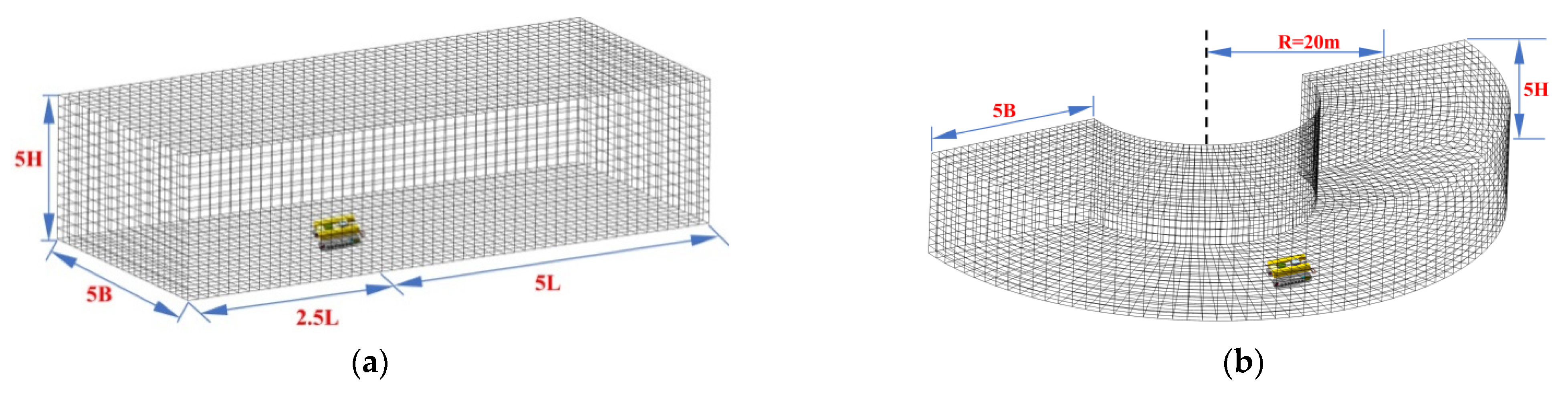
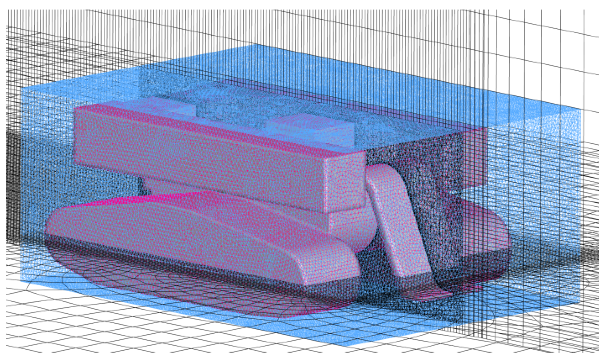
2.2.1. Meshing Method

The overset grid method was adopted to describe the actual working conditions of the mining vehicle. Benek et al. [30] described the overset grid approach to resolve the complex geometries flows, and its powerful potential for simulating complex engineering flows was demonstrated [31]. Then, the pressure coefficient was calculated to verify the accuracy of the calculation on the surface of the airfoil [32]. The overset grid method can significantly describe the movement of components and ensure the quality of grids in the simulation process.

2.2.2. Simulation Setup Details

The length, width, and height (L, W, and H) of the deep-sea mining vehicle are 5.4, 3.5, and 1.9 m, respectively. Therefore, the flow field areas shown in Figure 5 were established to simulate the spatial hydrodynamic distribution of straight motion and steering motion in ANSYS Fluent. The RNG k-ε turbulence model was selected, and the value of y⁺ was set as 30. As illustrated in Figure 6, each motion simulation included a background mesh and a component mesh, the former was generated by a multizone algorithm, and the latter was generated by an automatic algorithm. The flow field area established in Figure 5 can ensure the full development of the flow field during the simulation process, so all the boundary conditions of the flow field were set to the wall. The velocity of component mesh was set to 0–1.2 m/s in straight motion and 0–0.06 rad/s in steering motion. The flow field material was marine water with a density and dynamic viscosity of 1026 kg/m³ and 0.00103 kg/m·s, respectively.

For the study of grid independence, three simulation models with different numbers of grids were compared. The speed of straight motion and steering motion was set to 1.0 m/s and 0.05 rad/s, respectively. The discriminating ratio $R_g$ could be used to estimate the grid convergence by a grid triplet [33]. The $R_g$ is given by:

$$R_g=\frac{{\varphi }_1-{\varphi }_2}{{\varphi }_2-{\varphi }_3}$$

(3)

where ${\varphi }_1$, ${\varphi }_2$, and ${\varphi }_3$ are the solutions simulated by the fine, medium, and coarse mesh.

The simulated solutions for the three meshes are shown in

Table 2. Verification of convergence.

Mesh	Straight Motion		Steering Motion
	Number of Grids	longitudinal Resistance(N)	Number of Grids	longitudinal Resistance(N)
Coarse	3.2 million	3626.37	4.4 million	5016.49
Medium	4.5 million	3386.89	5.7 million	4821.83
Fine	5.6 million	3327.52	6.9 million	4751.35
Discriminating ratio		0.248		0.362

. It could be found that in straight and steering motions, all the R were in the range of 0–1. This indicated that with the increases in the number of grids, the convergence was monotonic convergence. Owing to the consideration of calculation time and accuracy, the medium mesh was selected.

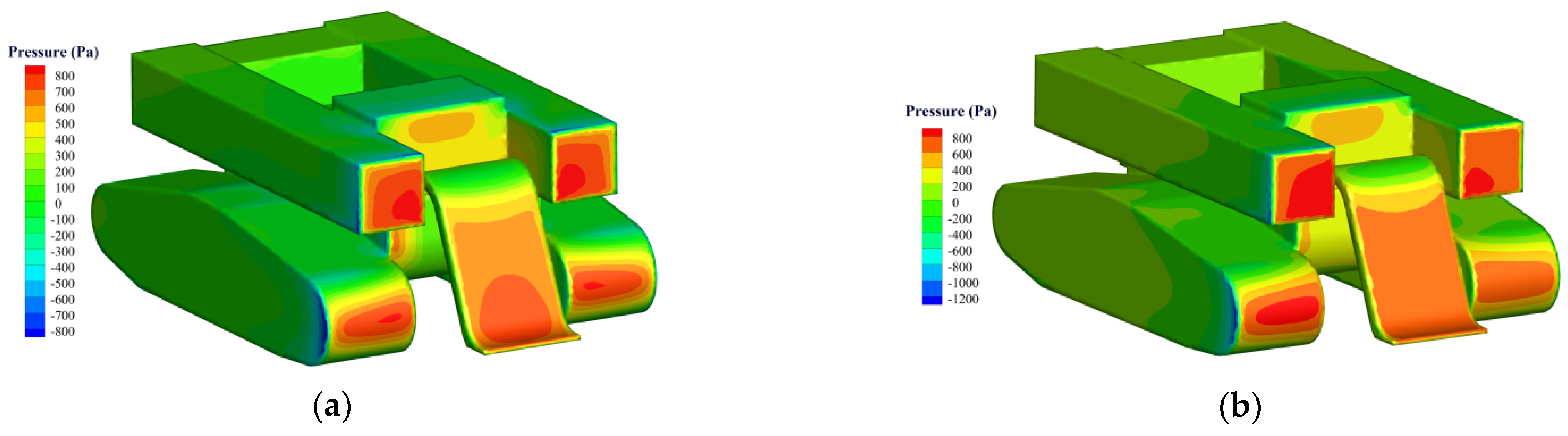
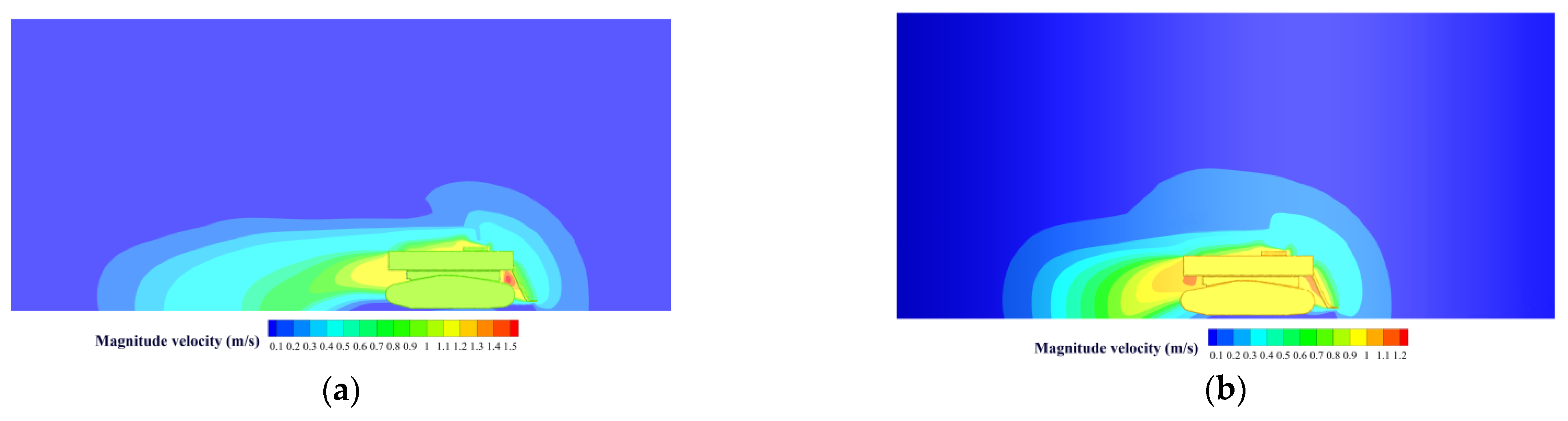
2.2.3. Simulation Results

The straight motion at 0–1.2 m/s and the steering motion at 0–0.06 rad/s of the mining vehicle were simulated and solved. The surface pressure distribution of the vehicle and velocity distributions of the flow field at 1 m/s and 0.05 rad/s are shown in Figure 7 and Figure 8, respectively. When the mining vehicle moved in a straight line, it is mainly subjected to longitudinal hydrodynamic resistance F_long, which mainly comes from the pressure difference between the front and rear surfaces of the vehicle. Moreover, the pressure on the left and right surfaces was roughly the same so that the lateral hydrodynamic resistance F_lat could be ignored. However, the F_lat was unable to be ignored with the asymmetry of the flow field in steering motion; the pressure difference would appear on the left and right surfaces of the mining vehicle. The F_long and F_lat are displayed in Figure 9 with their polynomial curves fitting.

The resistance of underwater moving objects is given by:

$$F=\frac{1}{2}{C}_{\mathrm{d}}\rho {\nu }^{2}A$$

(4)

where $C_{\mathrm{d}}$ is the coefficient of water resistance, $\rho$ is the density of seawater, $\nu$ is the speed of motion, and $A$ is the waterfront area.

As shown in Figure 9, the F_long and F_lat are proportional to the square of the speed, which is in line with the relationship between force and speed in Equation (4). In the MBD model, they would be applied at the corresponding positions with the form of axis force.

2.3. MBD Model

As shown in Figure 10, an equal scale MBD model of the deep-sea mining vehicle was established in multi-body dynamic simulation software Recurdyn, which is very suitable for solving large-scale multi-body system dynamics problems with relative coordinate system motion equation theory and fully recursive algorithm. The MBD model consisted of six parts, namely the collection device, the collection bin, the buoyancy material, the main frame, the left track, and the right track. They were all regarded as rigid bodies for simulation, and fixed constraints were imposed between the main frame and other parts. Among them, the track parts were established by subsystem tookit of track in recurdyn; all the contact forces were determined by the corresponding stiffness coefficient, damping coefficient, and dynamic friction coefficient. The spring connection was applied between the tensioner and the track frame, and all the wheels and track frame were restrained by rotating pairs. In addition, the track–surface contact was applied to the track and the ground. In this model, hydrodynamic resistance forces were applied separately in the X-axis and Y-axis directions to simulate the impact of ocean currents and changed with the movement speed, and the effect of cables and flexible risers were neglected to simplify the model. Simultaneously, C language was used to develop a program of the vehicle–sediment mechanical interaction with user subroutine in Recurdyn.

In the MBD model, base speed $u$ and the additional speed ratio $i$ would be input, and then, they were applied to control the left track speed $u_l$ and right track speed $u_r$. The relationships are given by:

$$\{\begin{array}{c}{u}_l=u(1-i)\\ u_r=u(1+i)\end{array}.$$

(5)

The movement diagram of the mining vehicle is shown in Figure 11; its central coordinates are ($X_{\mathrm{o}}$,$Y_{\mathrm{o}}$). Desired trajectories give the excepted path for straight and steering motion. The central coordinates of the circle ($X_{\mathrm{a}}$,$Y_{\mathrm{a}}$) and radius R are indicated. Wherein $e$ is the path-tracking error, $\alpha$ is the path-angle error, $\beta$ is the actual heading angle of the mining vehicle, and $\theta$ is the excepted angle. The corresponding relationships in straight motion are given by:

$$\{\begin{array}{l}e=\frac{\left|k{X}_o-Y_o\right|}{\sqrt{k^2+1}}\times \mathrm{sgn}(k-\frac{Y_o}{X_o})\hfill \\ \alpha =\theta -\beta \hfill \\ k=\tan \theta \hfill \end{array}.$$

(6)

The corresponding relationships in steering motion are given by:

$$\{\begin{array}{l}e=\left[\sqrt{{\left(X_o-X_a\right)}^2+{\left(Y_o-Y_a\right)}^2}-R\right]\times \mathrm{sgn}(\cos \theta )\hfill \\ \alpha =\frac{\pi }{2}-\theta -\beta \hfill \end{array}.$$

(7)

During the simulation process, the central coordinates and actual heading angle of the mining vehicle will be used to calculate path-tracking error and path-angle error, which are fed back to the control system in real time.

During the walking of the vehicle, the traction force mainly comes from the shear stress generated by the sediment during the interaction between the track belt and the sediment, which in turn was related to the shear displacement. In the process of walking, there will be a certain gap between its actual speed and the speed given by the controller. Due to the inflexibility of the track, it can be considered that the slip rate of each point of the track section is basically the same. The slip rate of track is given by:

$$i=\frac{v_s-v_m}{v_s}$$

(8)

where $v_s$ is the theoretical input speed of track, $v_m$ is the actual speed of track, and $i$ is the slip rate.

3. Exploration of the Path-Tracking Controller

Fuzzy logic control is widely used in marine robotic fields [34]; its performance is mainly affected by fuzzy rules. The design of fuzzy rules is often influenced by the experience limitations of the designer, which may lead to reduced control performance. The introduction of a genetic algorithm to optimize fuzzy rules can significantly eliminate the influence of subjective factors on the control performance.

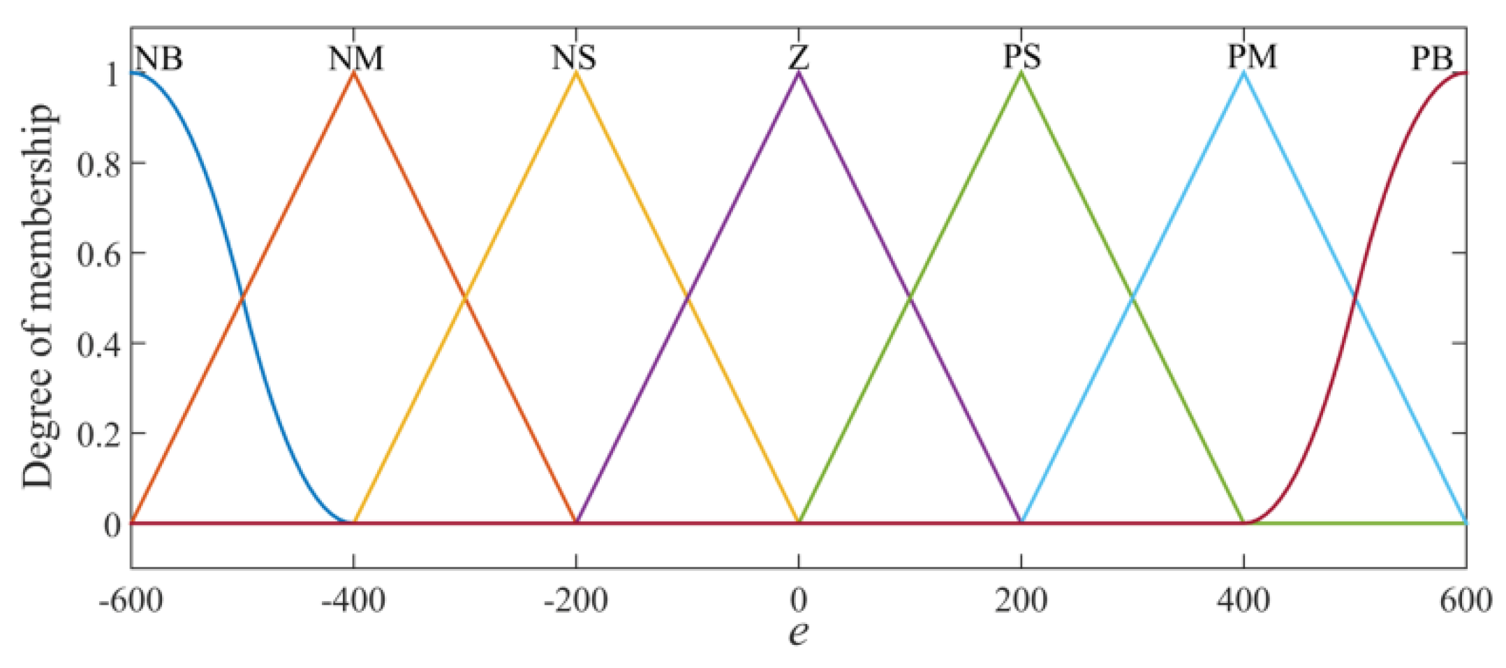
3.1. Design of Fuzzy Controller

A Mamdani-style fuzzy controller [35] was designed for path-tracking control of the mining vehicle, where the input parameters are the path-tracking error and path-angle error, and the output parameters are the base speed and additional speed ratio. The domains of $e$, $\alpha$, $u$, and $i$ are [−600 mm, 600 mm], [−6°, 6°], [0.5 m/s, 1.1 m/s], and [−0.3, 0.3], respectively; all of them have seven language variable values defined as NB, NM, NS, Z, PS, PM, and PB. As is shown in Figure 12, the type of z and s membership functions were used in NB and PB respectively, and the triangular membership function was applied in other language variable values. The other parameters used the same design form of the degree of membership function in Figure 12.

When both types of error are small, the base speed of the mining vehicle can be increased, and vice versa, it needs to be reduced. At the same time, the path-tracking error has more influence than the angle error for an additional speed ratio; when the absolute value of the path-tracking error is large, the additional speed ratio should be set to a large value and have the same language direction as the former. Similarly, when the absolute value of the path-tracking error is small, the additional speed ratio is also small. Based on the above empirical experience, the fuzzy rules demonstrated in

Table 3. The rules of base speed in the fuzzy controller.

$\mathit{e}\mathit{\alpha }$	NB	NM	NS	Z	PS	PM	PB
NB	NB	NM	NS	Z	Z	Z	NS
NM	NM	Z	Z	PS	PS	PS	Z
NS	NS	Z	Z	PM	PM	PS	Z
Z	Z	PS	PM	PB	PM	PS	Z
PS	Z	PS	PM	PM	Z	Z	NS
PM	Z	PS	PS	PS	Z	Z	NM
PB	NS	Z	Z	Z	NS	NM	NB

and

Table 4. The rules of additional speed ratio in the fuzzy controller.

$\mathit{e}\mathit{\alpha }$	NB	NM	NS	Z	PS	PM	PB
NB	NB	NB	NM	NS	NS	NS	Z
NM	NB	NM	NS	NS	NS	NS	Z
NS	NM	NS	NS	Z	Z	Z	Z
Z	NM	NM	NS	Z	PS	PM	PM
PS	Z	Z	Z	Z	PS	PS	PM
PM	Z	PS	PS	PS	PS	PM	PB
PB	Z	PS	PS	PS	PM	PB	PB

were created, and the centroid strategy was applied in defuzzification.

.

3.2. Optimization of Fuzzy Controller

As for a global search algorithm, a genetic algorithm can obtain the global optimal solution of an optimization problem. First of all, it is essential to decide the decision variables and constraints according to the optimization problem and then establish an optimization model and objective function. Second, the encoding and decoding methods need to be determined. Finally, the individual evaluation method and relevant operating parameters should be defined.

In this study, a total of 98 parameters need to be optimized in Table 3 and Table 4; and all the parameters are integers. The value range is [1,7], which is equivalent to [NB, NM, NS, Z, PS, PM, PB] in the optimization process. The genetic algorithm named MI-LXPM was applied to resolve this optimized problem for its efficiency in integer-constrained optimization problems [36,37], and real encoding was adopted. In the movement of the mining vehicle, the smallest path-tracking error is expected, and the objective function is given by:

$$\min f(e)=\sqrt{\frac{{\displaystyle \sum _{i=1}^n{e}_i{}^2}}{n}}.$$

(9)

The optimization function in the genetic algorithm always minimizes the fitness function, so in the minimum objective function, the fitness function is given by:

$$Fit(f(e))=\frac{1}{1+m-f(e)}, m\ge 0, m-f(e)\ge 0$$

(10)

where $m$ is the bounds of the objective function with conservative estimation, and its value is set to 3.

The crossover operator and mutation operator are the most critical parameters of the genetic optimization algorithm, which work together to perform a global search and a local search of the search space. The values of the crossover operator and mutation operator were taken as 0.8 and 0.05 to ensure that the genetic algorithm has good search performance.

The fuzzy controller was established in MATLAB/Simulink, so it could be optimized by a genetic algorithm through the co-simulation between the controller and the MBD model. The co-simulation process of Simulink and Recurdyn is depicted in Figure 13.

When the co-simulation was running, the genetic algorithm would update the parameters according to the fitness function values in each iteration until it met the iteration conditions and given the best parameter value. The optimization flow chart is manifested in Figure 14.

After 239 generations, the optimal parameters were acquired, and the rules of the optimized fuzzy controller are shown in

Table 5. The rules of base speed in the optimized fuzzy controller.

$\mathit{e}\mathit{\alpha }$	NB	NM	NS	Z	PS	PM	PB
NB	NB	NB	NM	Z	Z	NS	NS
NM	NM	NS	NS	PS	PS	Z	NS
NS	NM	Z	Z	PS	PS	PS	Z
Z	Z	PS	PM	PB	PM	PS	Z
PS	Z	PS	PS	PS	Z	Z	NM
PM	NS	Z	PS	PS	NS	NS	NM
PB	NS	NS	Z	Z	NM	NB	NB

and

Table 6. The rules of additional speed ratio in the optimized fuzzy controller.

$\mathit{e}\mathit{\alpha }$	NB	NM	NS	Z	PS	PM	PB
NB	NB	NB	NM	NS	NS	NS	Z
NM	NB	NM	NS	NS	NS	NS	Z
NS	NM	NS	NS	Z	Z	Z	Z
Z	NM	NM	NS	Z	PS	PM	PM
PS	Z	Z	Z	Z	PS	PS	PM
PM	Z	PS	PS	PS	PS	PM	PB
PB	Z	PS	PS	PS	PM	PB	PB

.

3.3. Simulation Results of Two Controllers

The fuzzy control optimized by the genetic algorithm was obtained. Then, the collaborative motion simulation of the path tracking was carried out. The curve of the expected path in the co-simulation was defined as (Unit:m):

$$\{\begin{array}{c}y=0,0\le x\le 20\\ {(x-20)}^2+{(y-20)}^2=400,x>20\\ y=40,0\le x\le 20\end{array}.$$

(11)

The change of the Z-direction position was ignored, and the mining vehicle forwarded along the positive direction of the X-axis. We found that both controllers were capable of path tracking from the simulation results displayed in Figure 15. In linear motion, the trajectory of the actual motion almost coincides with the expected path. In contrast, in the steering motion, the turning radius of the actual motion trajectory will be larger than the radius of the expected path, and the path error was larger than when driving in a straight line. However, compared with the original fuzzy controller, the optimized fuzzy controller has better control accuracy.

In the simulation process, the left track speed $u_l$ and right track speed $u_r$ of MBD model in Figure 16 were continuously changed by the optimized fuzzy controller to adjust the path error and obtain a better control performance. During straight and steering motion, the $u_l$ and $u_r$ were maintained near a more stable value; while in the transition period of the motion state, there would be a quick adjustment. It can be found that the optimized fuzzy controller has excellent ability to control the track speed in the straight and steering motion in a complex seabed environment.

Figure 17 indicated the velocity of the mining vehicle. In the beginning of the motion, the responding speed of the optimized fuzzy control performed better than the original one, and there was less fluctuation with the optimized fuzzy controller in case of the large sudden interference. It was evident that the stability of the velocity using the original fuzzy controller was not as good as that of the optimized fuzzy controller.

Figure 18 demonstrated the path-tracking error of the simulation process. The largest path-tracking error was 214 mm with the optimized fuzzy controller, while without optimization, the largest path-tracking error was 598 mm. The latter path-tracking error varied more sharply throughout the motion. Figure 19 indicated the path-angle error. The path-angle error was small in the straight motion and large in the steering motion. It was clear that the optimized fuzzy controller has better control performance, with a smaller maximum angle error and fluctuation.

The path-tracking error and the path-angle error were changed continuously in the motion process of the mining vehicle, so the reference velocities that were used to control the left track and right track would change at the same time according to the control rules of the fuzzy controller. The slip rate of the left and right tracks in the movement process is shown in Figure 20. At the beginning of the straight motion, the slip rate fluctuations were small, and the vehicle was in a relatively stable state; in the subsequent steering motion, the slip rate fluctuated more, which meant that the stability of the steering motion was not as good as the straight process, and more frequent and greater adjustments were required to reduce the path error; when the car completed the steering motion and entered the straight motion again, the slip rate of the track was also maintained in a smaller fluctuation range. In the whole motion process, the slip rate of the crawler was between 0 and 0.03 most of the time. The slip rate in this interval could provide the vehicle with greater traction and obtained a higher energy efficiency.

From the above simulation results, there was no doubt that the optimized fuzzy controller has achieved the path-tracking control of the deep-sea mining vehicle. Furthermore, its control accuracy and stability, which fully met the design requirements, had been significantly improved compared to the controller designed by human experience. The genetic algorithm could develop a satisfactory fuzzy controller for the mining vehicle, as long as a suitable dynamic model was established ahead.

4. Conclusions

An integrated dynamic model and optimized fuzzy controller for the path tracking of a deep-sea mining vehicle were studied. In this paper, we have simplified some research; in the future, the study of hydrodynamics in more complex situations such as uphill, downhill, and ditch crossing, and the deeper coupling between the vehicle and the cable could be considered. The major results of this paper are as follows:

(1)

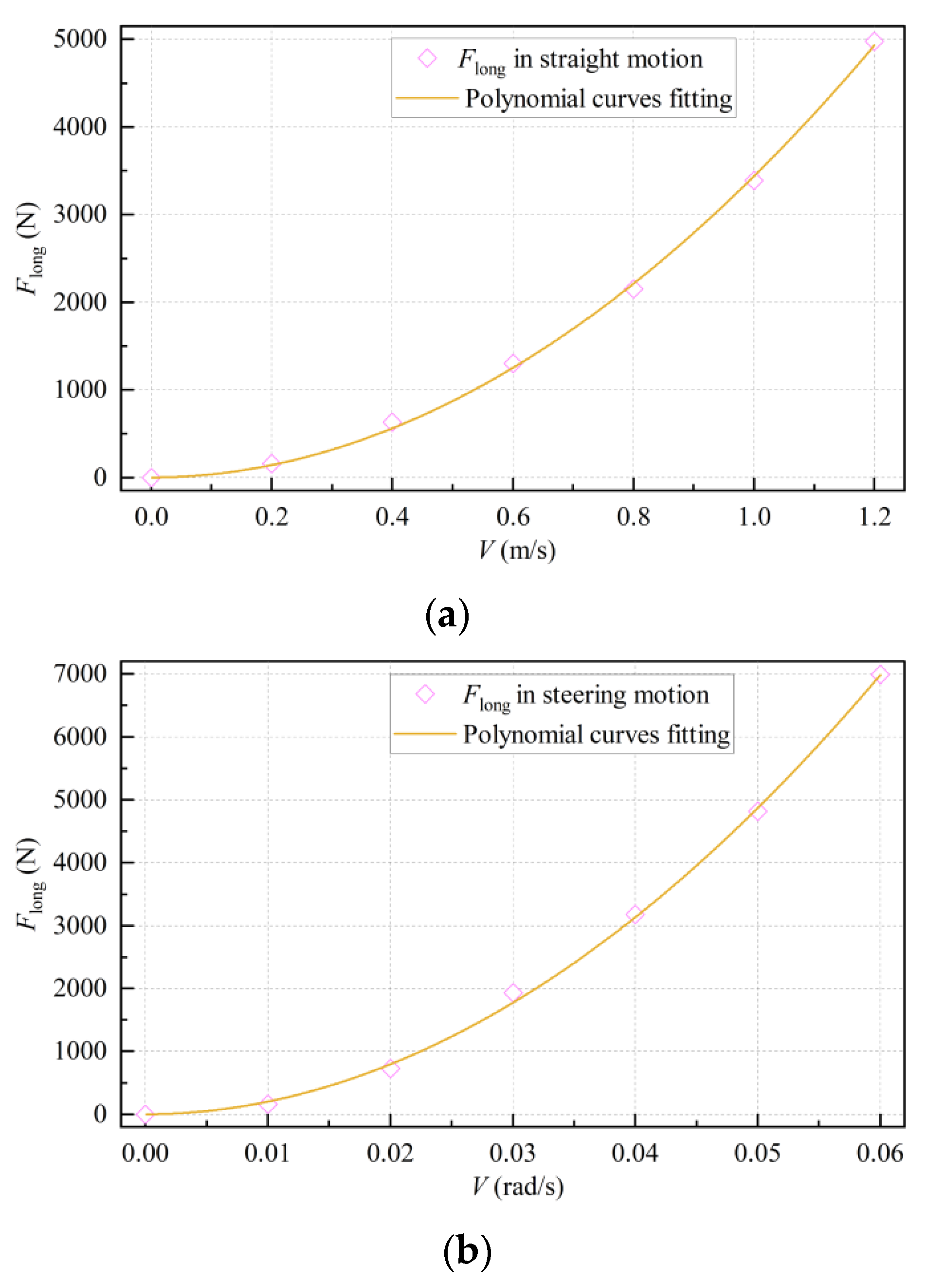
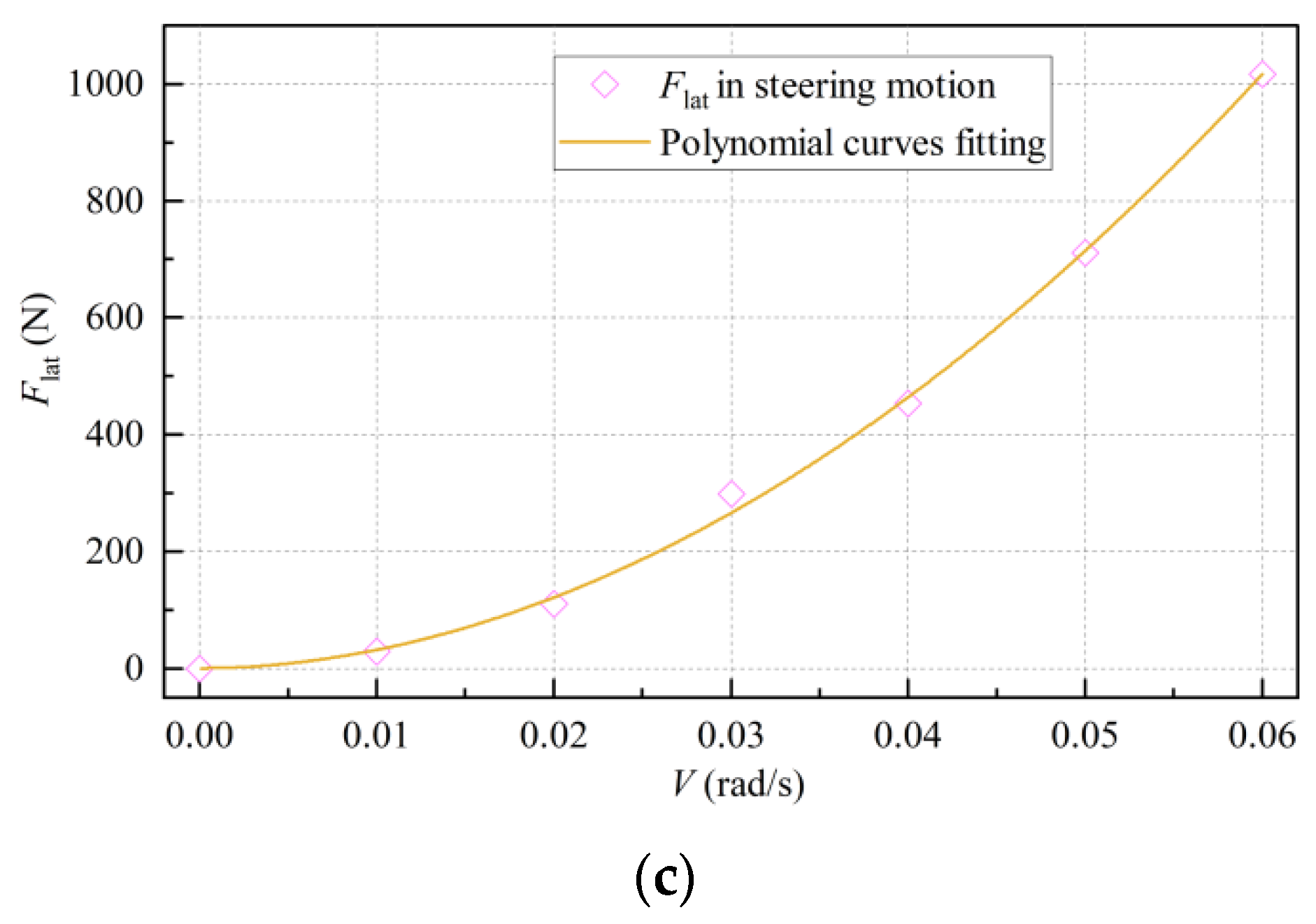
The related parameters of vehicle–sediment mechanical interaction were calculated by sinkage and shear tests in the laboratory, and the trends of test data were highly consistent with corresponding empirical equations. The longitudinal hydrodynamic resistance and lateral hydrodynamic resistance of the mining vehicle increased exponentially with the increase of speed; simultaneously, the lateral hydrodynamic resistance of straight motion was too small to be ignored.

(2)

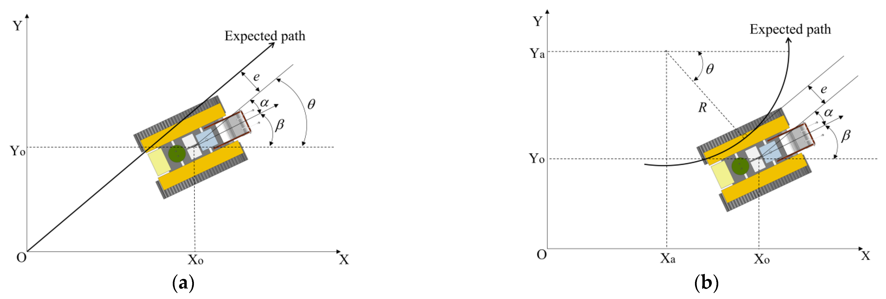
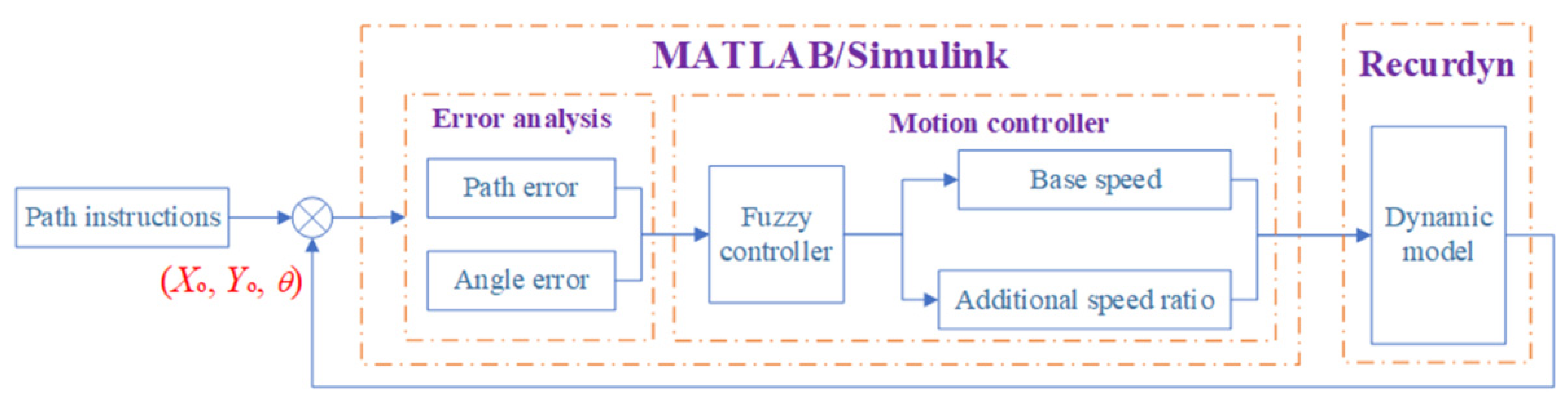
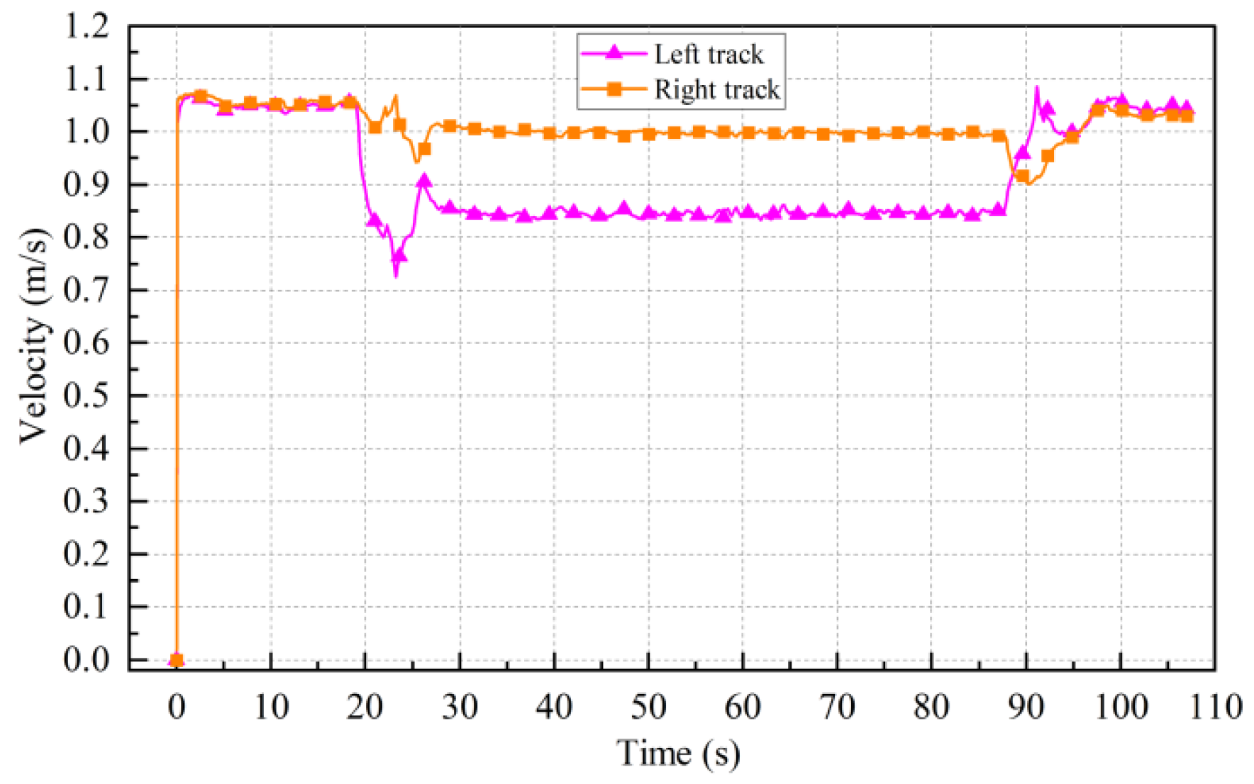
The MBD model of the deep-sea mining vehicle utilized axis forces and a user subroutine to achieve the integration of the mechanical interaction between vehicle and sediment and the spatial hydrodynamic effects. The central coordinates and actual heading angle of the mining vehicle were sampled in real time to calculate the path-tracking error and path-angle error in different motion states.

(3)

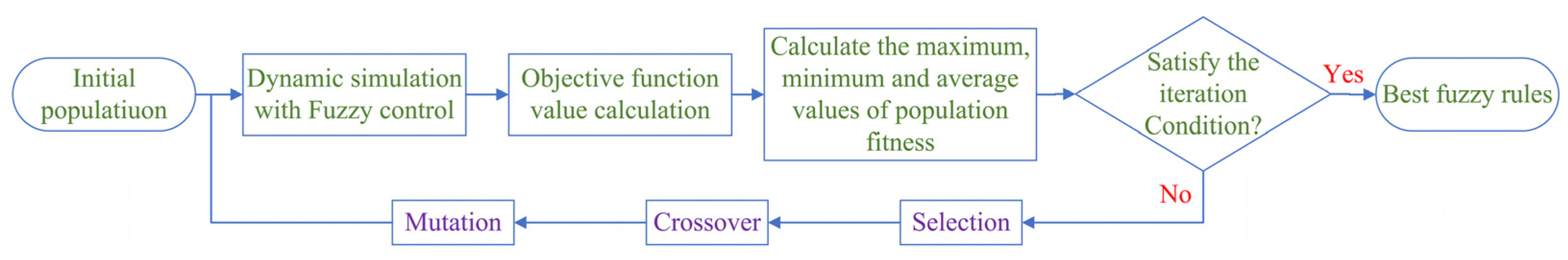
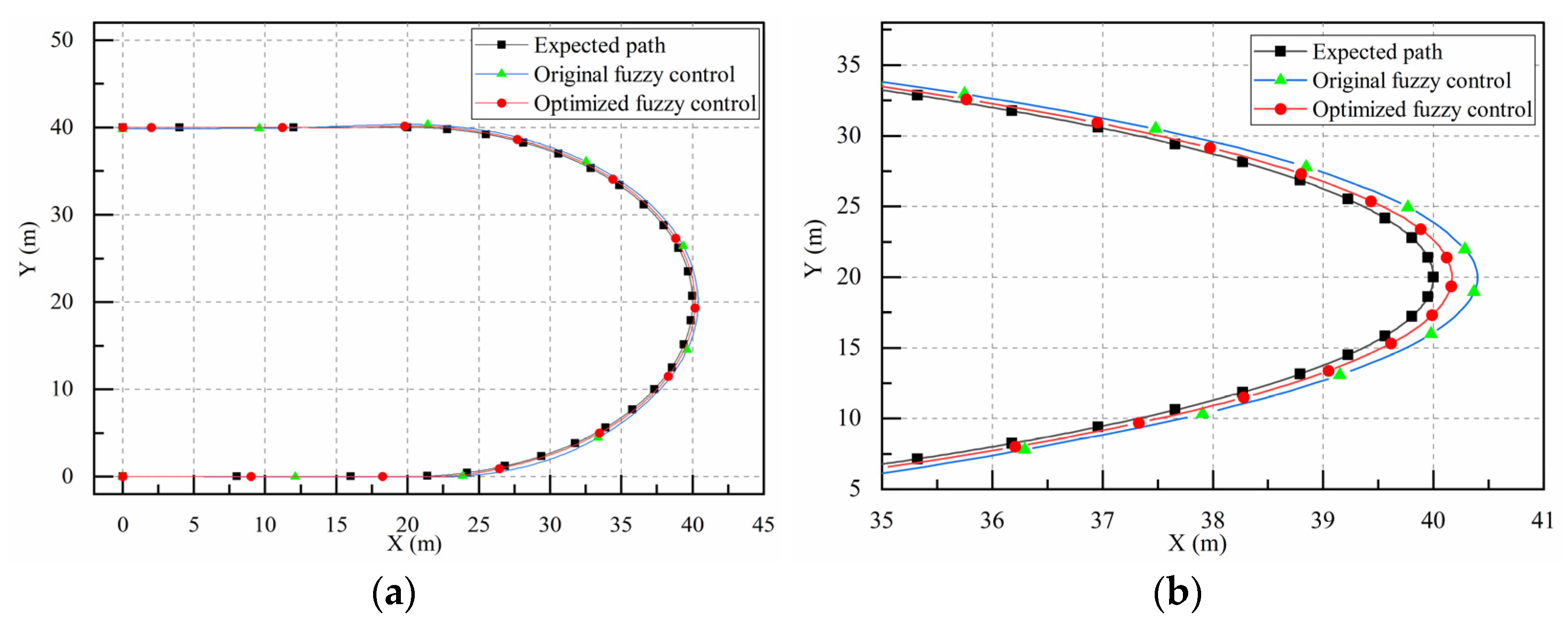
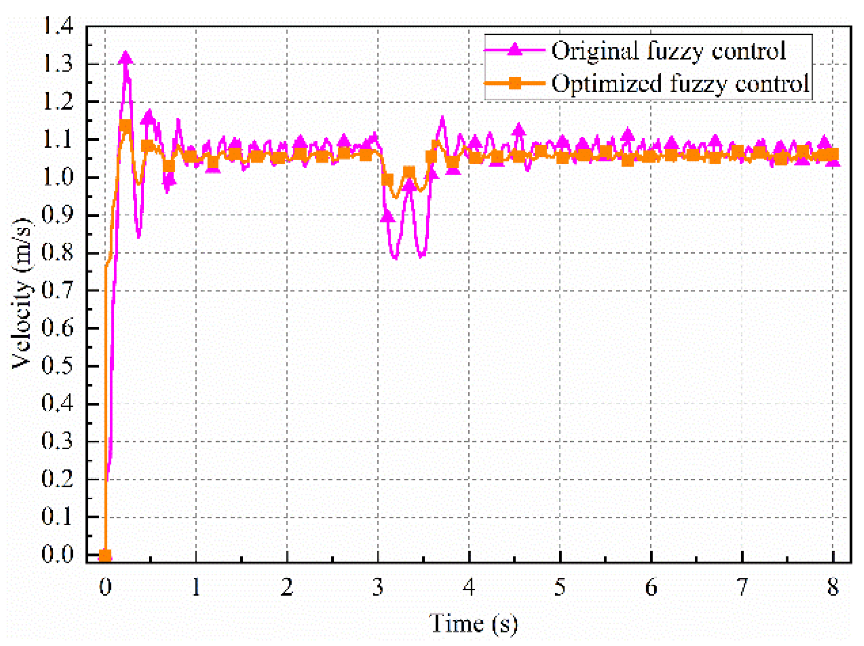
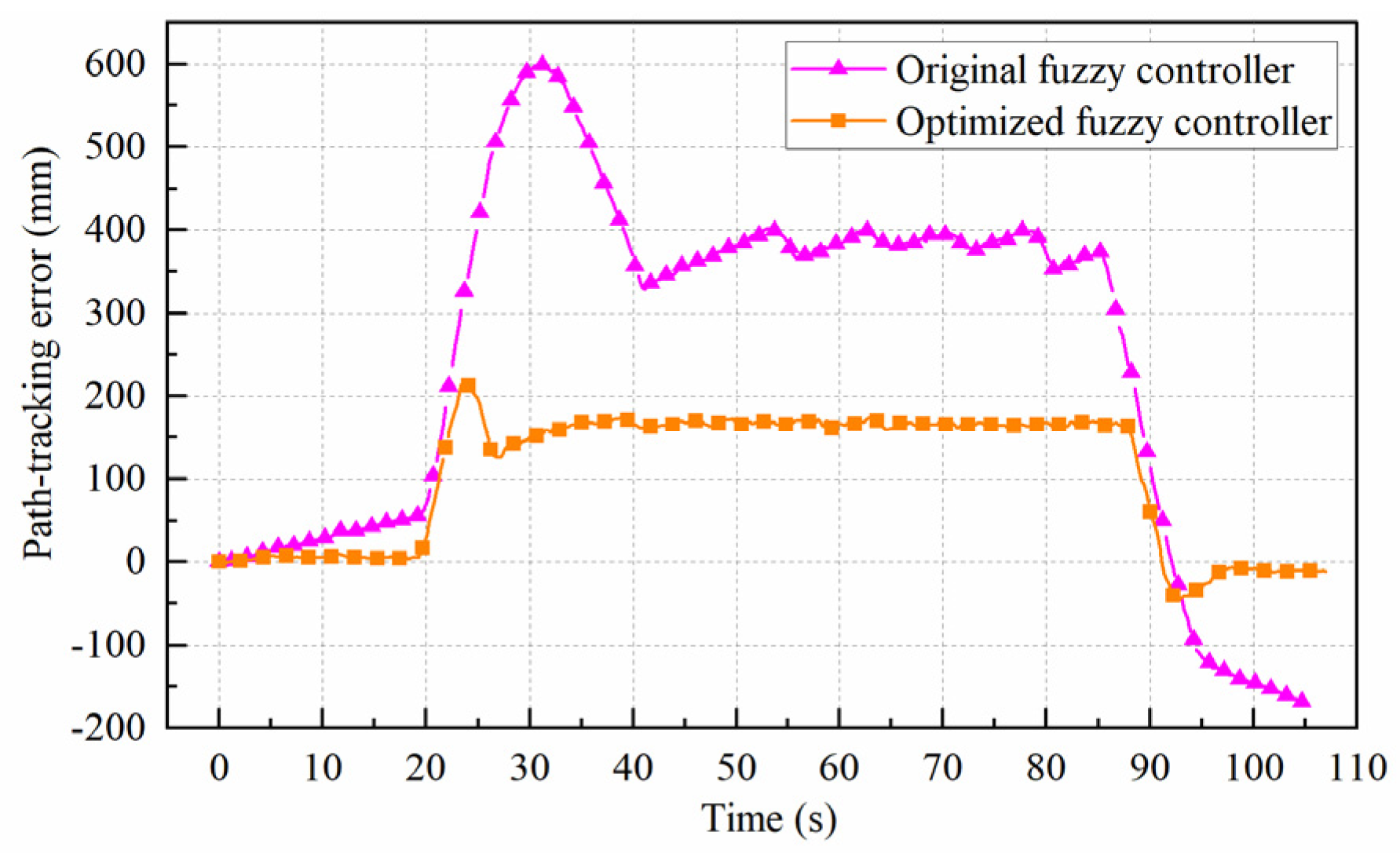
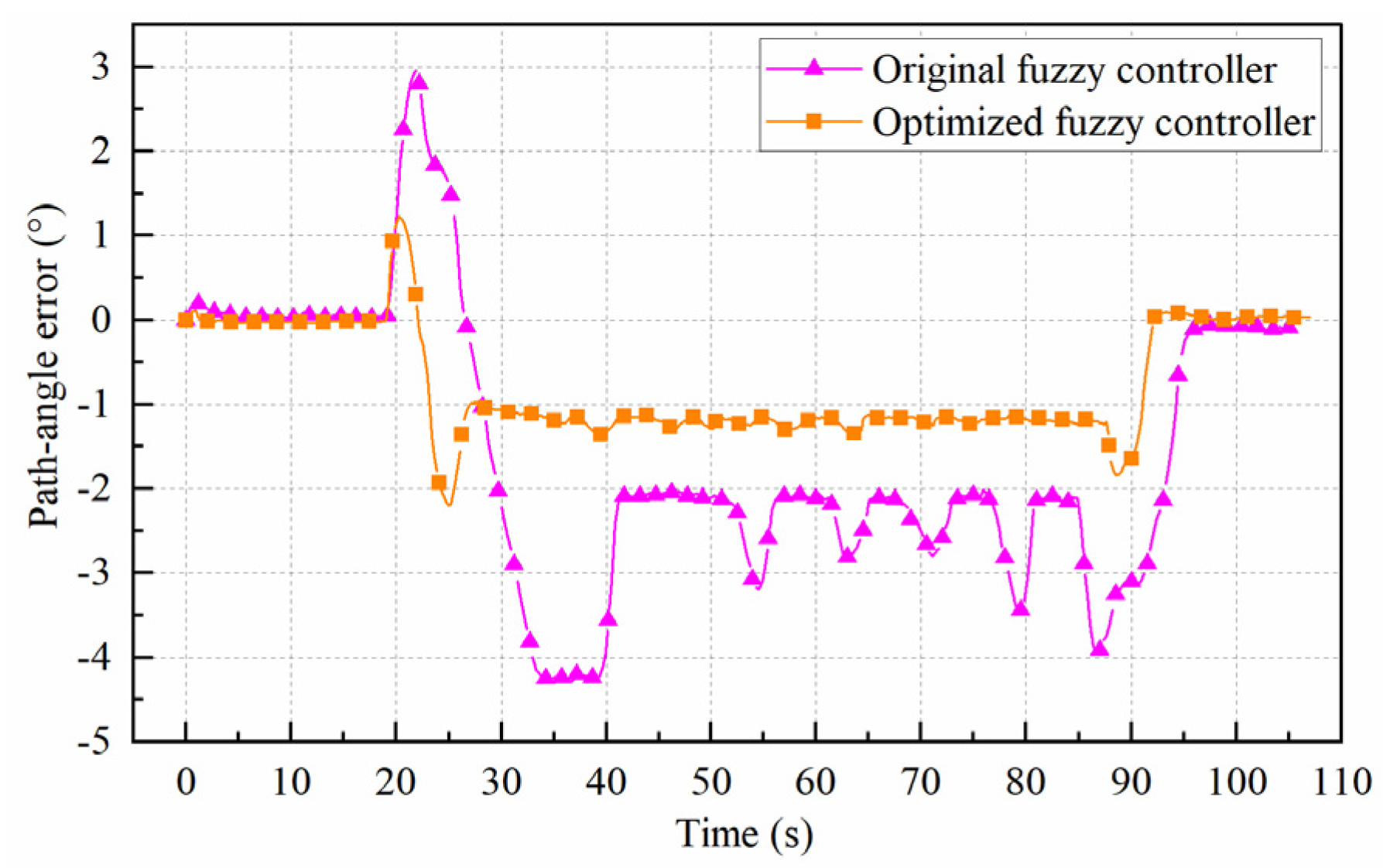
The genetic algorithm named MI-LXPM optimized the fuzzy rules of the motion controller. The co-simulation showed that the optimized fuzzy controller had better control accuracy than the original fuzzy controller. The maximum path-tracking error and path-angle error of the optimized fuzzy controller were 214 mm and −2.1°, respectively, but the corresponding values of the original fuzzy controller were 598 mm and −4.3°.

References

1. Chung, J.S. Deep-Ocean Mining Technology III: Developments. Eighth ISOPE Ocean Mining Symposium; International Society of Offshore and Polar Engineers: Chennai, India, 2009; p. 7. [Google Scholar]
2. Hong, S.; Kim, H.W.; Choi, J.S. Transient dynamic analysis of tracked vehicles on extremely soft cohesive soil. In Proceedings of the Fifth (2002) Isope Pacific/Asia Offshore Mechanics Sympopsium, Daejeon, Korea, 17–20 November 2002; pp. 100–107. [Google Scholar]
3. Kim, H.W.; Hong, S.; Choi, J.; Yeu, T.K. Dynamic analysis of underwater tracked vehicle on extremely soft soil by using Euler parameters. In Proceedings of the Sixth (2005) Isope Ocean Mining Symposium, Changsha, China, 9–13 October 2005; pp. 141–148. [Google Scholar]
4. Kim, H.W.; Hong, S.; Choi, J.S. Comparative study on tracked vehicle dynamics on soft soil: Single-body dynamics vs. multi-body dynamics. In Proceedings of the Fifth (2003) Isope Ocean Mining Symposium, Tsukuba, Japan, 15–19 September 2003; pp. 132–138. [Google Scholar]
5. Dai, Y.; Liu, S.-J. An integrated dynamic model of ocean mining system and fast simulation of its longitudinal reciprocating motion. China Ocean Eng. 2013, 27, 231–244. [Google Scholar] [CrossRef]
6. Jagadeesh, P.; Murali, K.; Idichandy, V. Experimental investigation of hydrodynamic force coefficients over AUV hull form. Ocean Eng. 2009, 36, 113–118. [Google Scholar] [CrossRef]
7. Phillips, A.B.; Turnock, S.R.; Furlong, M. The use of computational fluid dynamics to aid cost-effective hydrodynamic design of autonomous underwater vehicles. Proc. Inst. Mech. Eng. Part M J. Eng. Marit. Environ. 2010, 224, 239–254. [Google Scholar] [CrossRef]
8. Chin, C.S.; Lin, W.P.; Lin, J.Y. Experimental validation of open-frame ROV model for virtual reality simulation and control. J. Mar. Sci. Technol. 2017, 23, 267–287. [Google Scholar] [CrossRef] [Green Version]
9. Vu, M.T.; Choi, H.-S.; Kim, J.-Y.; Tran, N.H. A study on an underwater tracked vehicle with a ladder trencher. Ocean Eng. 2016, 127, 90–102. [Google Scholar] [CrossRef]
10. Vu, M.T.; Choi, H.-S.; Ji, D.H.; Jeong, S.-K.; Kim, J.-Y. A study on an up-milling rock crushing tool operation of an underwater tracked vehicle. Proc. Inst. Mech. Eng. Part M J. Eng. Marit. Environ. 2019, 233, 283–300. [Google Scholar] [CrossRef]
11. Li, J.; Dai, Y.; Liu, S. Effect of grouser height on tractive performance of tracked mining vehicle. J. Braz. Soc. Mech. Sci. Eng. 2016, 39, 2459–2466. [Google Scholar] [CrossRef]
12. Wang, M.; Wang, X.; Sun, Y.; Gu, Z. Tractive performance evaluation of seafloor tracked trencher based on laboratory mechanical measurements. Int. J. Nav. Arch. Ocean Eng. 2016, 8, 177–187. [Google Scholar] [CrossRef] [Green Version]
13. Baek, S.-H.; Shin, G.-B.; Chung, C.-K. Experimental study on the soil thrust of underwater tracked vehicles moving on the clay seafloor. Appl. Ocean Res. 2019, 86, 117–127. [Google Scholar] [CrossRef]
14. Vu, M.T.; Choi, H.-S.; Nguyen, N.D.; Kim, S.-K. Analytical design of an underwater construction robot on the slope with an up-cutting mode operation of a cutter bar. Appl. Ocean Res. 2019, 86, 289–309. [Google Scholar] [CrossRef]
15. Sun, Y.; Zhang, C.; Zhang, G.; Xu, H.; Ran, X. Three-Dimensional Path Tracking Control of Autonomous Underwater Vehicle Based on Deep Reinforcement Learning. J. Mar. Sci. Eng. 2019, 7, 443. [Google Scholar] [CrossRef] [Green Version]
16. Dai, Y.; Li, X.; Yin, W.; Pang, L.; Xie, Y.; Huang, Z. Dynamic modelling and motion control research on deep seabed miner. Mar. Georesources Geotechnol. 2020, 1–9. [Google Scholar] [CrossRef]
17. Dai, Y.; Su, Q.; Zhang, Y. A new dynamic model and trajectory tracking control strategy for deep ocean mining vehicle. Ocean Eng. 2020, 216, 108162. [Google Scholar] [CrossRef]
18. Yeu, T.-K.; Park, S.-J.; Hong, S.; Kim, H.-W.; Choi, J.-S. Path Tracking using Vector Pursuit Algorithm for Tracked Vehicles Driving on the Soft Cohesive Soil. In Proceedings of the 2006 SICE-ICASE International Joint Conference, Busan, Korea, 18–21 October 2006; IEEE: Piscataway, NJ, USA, 2006; pp. 2781–2786. [Google Scholar]
19. Hong, S.; Choi, J.-S.; Kim, H.-W.; Won, M.-C.; Shin, S.-C.; Rhee, J.-S.; Park, H.-U. A path tracking control algorithm for underwater mining vehicles. J. Mech. Sci. Technol. 2009, 23, 2030–2037. [Google Scholar] [CrossRef]
20. Zhang, L.; Chen, J.-W.; Sun, Y.-X.; Hao, S. Path-following control of remotely operated vehicle based on improved hybrid fuzzy PID control. AER Adv. Eng. Res. 2016, 117, 800–806. [Google Scholar]
21. Londhe, P.; Mohan, S.; Patre, B.; Waghmare, L. Robust task-space control of an autonomous underwater vehicle-manipulator system by PID-like fuzzy control scheme with disturbance estimator. Ocean Eng. 2017, 139, 1–13. [Google Scholar] [CrossRef]
22. Lamraoui, H.C.; Qidan, Z. Path following control of fully-actuated autonomous underwater vehicle in presence of fast-varying disturbances. Appl. Ocean Res. 2019, 86, 40–46. [Google Scholar] [CrossRef]
23. Aras, M.S.M.; Abdullah, S.S. Adaptive Simplified Fuzzy Logic Controller for Depth Control of Underwater Remotely Operated Vehicle. Indian J. Geo-Mar. Sci. 2015, 44, 1995–2007. [Google Scholar]
24. Hu, X.; Du, J.; Shi, J. Adaptive fuzzy controller design for dynamic positioning system of vessels. Appl. Ocean Res. 2015, 53, 46–53. [Google Scholar] [CrossRef]
25. Chen, J.; Zhu, H.; Zhang, L.; Sun, Y. Research on fuzzy control of path tracking for underwater vehicle based on genetic algorithm optimization. Ocean Eng. 2018, 156, 217–223. [Google Scholar] [CrossRef]
26. Londhe, P.S.; Patre, B.M. Adaptive fuzzy sliding mode control for robust trajectory tracking control of an autonomous underwater vehicle. Intell. Serv. Robot. 2018, 12, 87–102. [Google Scholar] [CrossRef]
27. Dai, Y.; Zhu, X.; Zhou, H.; Mao, Z.; Wu, W. Trajectory Tracking Control for Seafloor Tracked Vehicle By Adaptive Neural-Fuzzy Inference System Algorithm. Int. J. Comput. Commun. Control. 2018, 13, 465–476. [Google Scholar] [CrossRef] [Green Version]
28. Bekker, M.G. Introduction to Terrain-Vehicle Systems; University of Michigan Press: Ann Arbor, MI, USA, 1969. [Google Scholar]
29. Wong, J.; Preston-Thomas, J. On the characterization of the shear stress-displacement relationship of terrain. J. Terramech. 1983, 19, 225–234. [Google Scholar] [CrossRef]
30. Benek, J.; Steger, J.; Dougherty, F. A flexible grid embedding technique with application to the Euler equations. In Proceedings of the 6th Computational Fluid Dynamics Conference, Danvers, MA, USA, 13–15 July 1983. [Google Scholar]
31. Tang, H.; Jones, S.C.; Sotiropoulos, F. An overset-grid method for 3D unsteady incompressible flows. J. Comput. Phys. 2003, 191, 567–600. [Google Scholar] [CrossRef]
32. Hoke, C.; Decker, R.; Cummings, R.; McDaniel, D.; Morton, S. Comparison of Overset Grid and Grid Deformation Techniques Applied to 2-Dimensional NACA Airfoils. In 19th AIAA Computational Fluid Dynamics; American Institute of Aeronautics and Astronautics: San Antonio, TX, USA, 2009. [Google Scholar]
33. Roache, P.J. Verification and Validation in Computational Science and Engineering; Hermosa Albuquerque: Albuquerque, NM, USA, 1998; Volume 895. [Google Scholar]
34. Xiang, X.; Yu, C.; Lapierre, L.; Zhang, J.; Zhang, Q. Survey on Fuzzy-Logic-Based Guidance and Control of Marine Surface Vehicles and Underwater Vehicles. Int. J. Fuzzy Syst. 2018, 20, 572–586. [Google Scholar] [CrossRef]
35. Mamdani, E.; Assilian, S. An experiment in linguistic synthesis with a fuzzy logic controller. Int. J. Man-Mach. Stud. 1975, 7, 1–13. [Google Scholar] [CrossRef]
36. Deep, K.; Thakur, M. A new crossover operator for real coded genetic algorithms. Appl. Math. Comput. 2007, 188, 895–911. [Google Scholar] [CrossRef]
37. Deep, K.; Singh, K.P.; Kansal, M.; Mohan, C. A real coded genetic algorithm for solving integer and mixed integer optimization problems. Appl. Math. Comput. 2009, 212, 505–518. [Google Scholar] [CrossRef]
Figure 1. Simulated sediment.
Jmse 09 00249 g001
Figure 2. Shear test process.
Jmse 09 00249 g002
Figure 3. Sinkage test data and fitting curve.
Jmse 09 00249 g003
Figure 4. Shear test data and fitting curve.
Jmse 09 00249 g004
Figure 5. The flow field areas: (a) straight motion; (b) steering motion.
Jmse 09 00249 g005
Figure 6. The background mesh and component mesh.
Jmse 09 00249 g006
Figure 7. The surface pressure distribution of mining vehicle: (a) straight motion at 1.0 m/s; (b) steering motion at 0.05 rad/s.
Jmse 09 00249 g007
Figure 8. The velocity distribution of flow field: (a) straight motion at 1.0 m/s; (b) steering motion at 0.05 rad/s.
Jmse 09 00249 g008
Figure 9. Hydrodynamic effects of the mining vehicle: (a) Flong and its polynomial curves fitting in straight motion; (b) Flong and its polynomial curves fitting in steering motion; (c) Flat and its polynomial curves fitting in steering motion.
Jmse 09 00249 g009aJmse 09 00249 g009b
Figure 10. The multi-body dynamic (MBD) model of mining vehicle.
Jmse 09 00249 g010
Figure 11. The movement diagram of the mining vehicle: (a) straight motion; (b) steering motion.
Jmse 09 00249 g011
Figure 12. The degree of membership function of e .
Jmse 09 00249 g012
Figure 13. Co-simulation process.
Jmse 09 00249 g013
Figure 14. The optimization flow chart.
Jmse 09 00249 g014
Figure 15. (a) The simulation results; (b) Partial enlargement of the simulation results.
Jmse 09 00249 g015
Figure 16. Velocity of left track and right track.
Jmse 09 00249 g016
Figure 17. Velocity of the mining vehicle.
Jmse 09 00249 g017
Figure 18. Path-tracking error of the simulation process.
Jmse 09 00249 g018
Figure 19. Path-angle error of the simulation process.
Jmse 09 00249 g019
Figure 20. Slip rate of the simulation process.
Jmse 09 00249 g020