
A Numerical Swallowing-Capacity Analysis of a Vacant, Cylindrical, Bi-Directional Tidal Turbine Duct in Aligned & Yawed Flow Conditions


Abstract
1. Introduction
2. Numerical Methodology
2.1. Physical Setup
2.2. Numerical Setup
3. Numerical Model Characterisation
3.1. Physical Modelling
3.2. CFD Modelling
3.2.1. Conservation Modelling
3.2.2. Turbulence Modelling
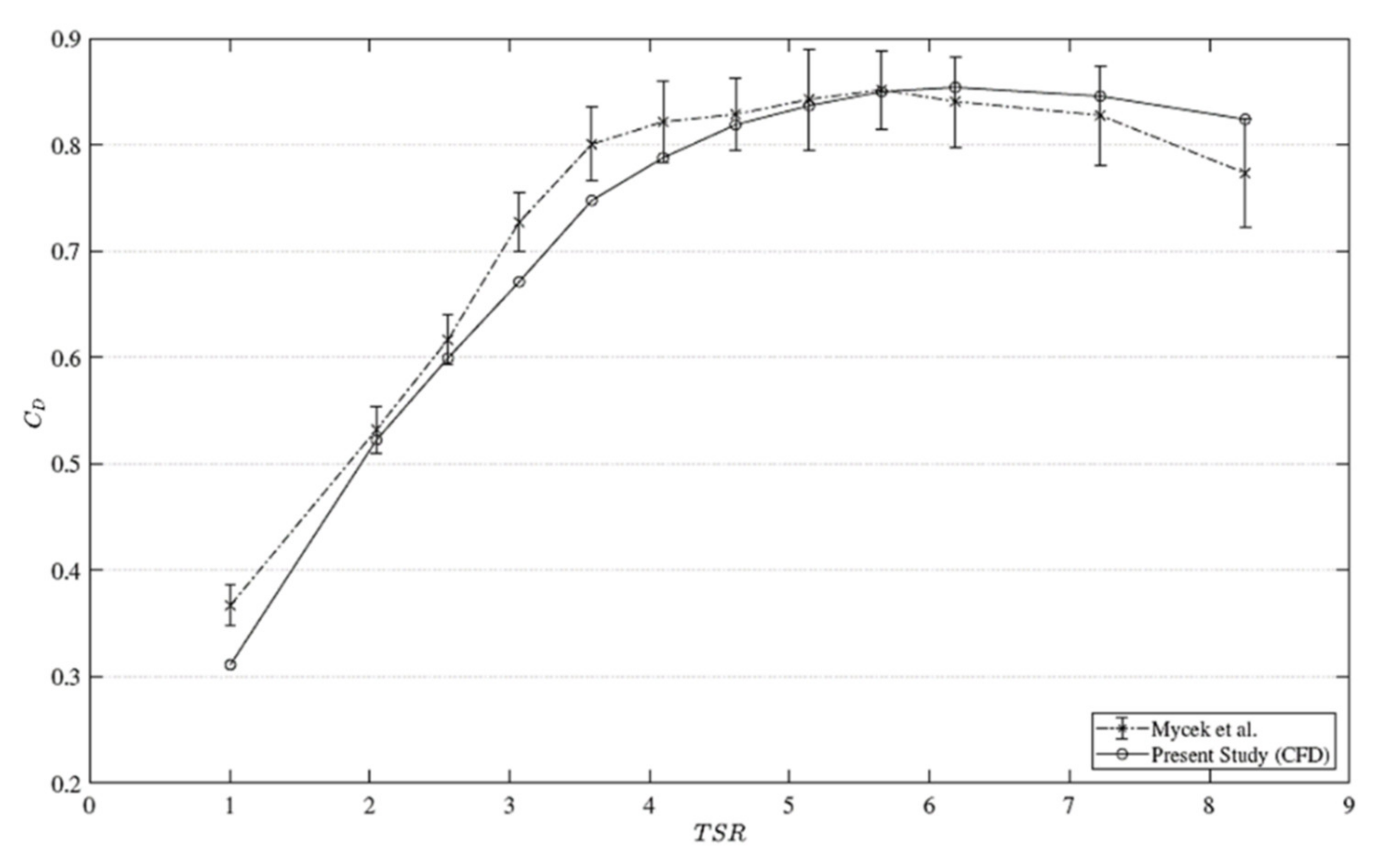
4. Modelling Validation
5. Vacant Duct Performance in Aligned Flow Conditions
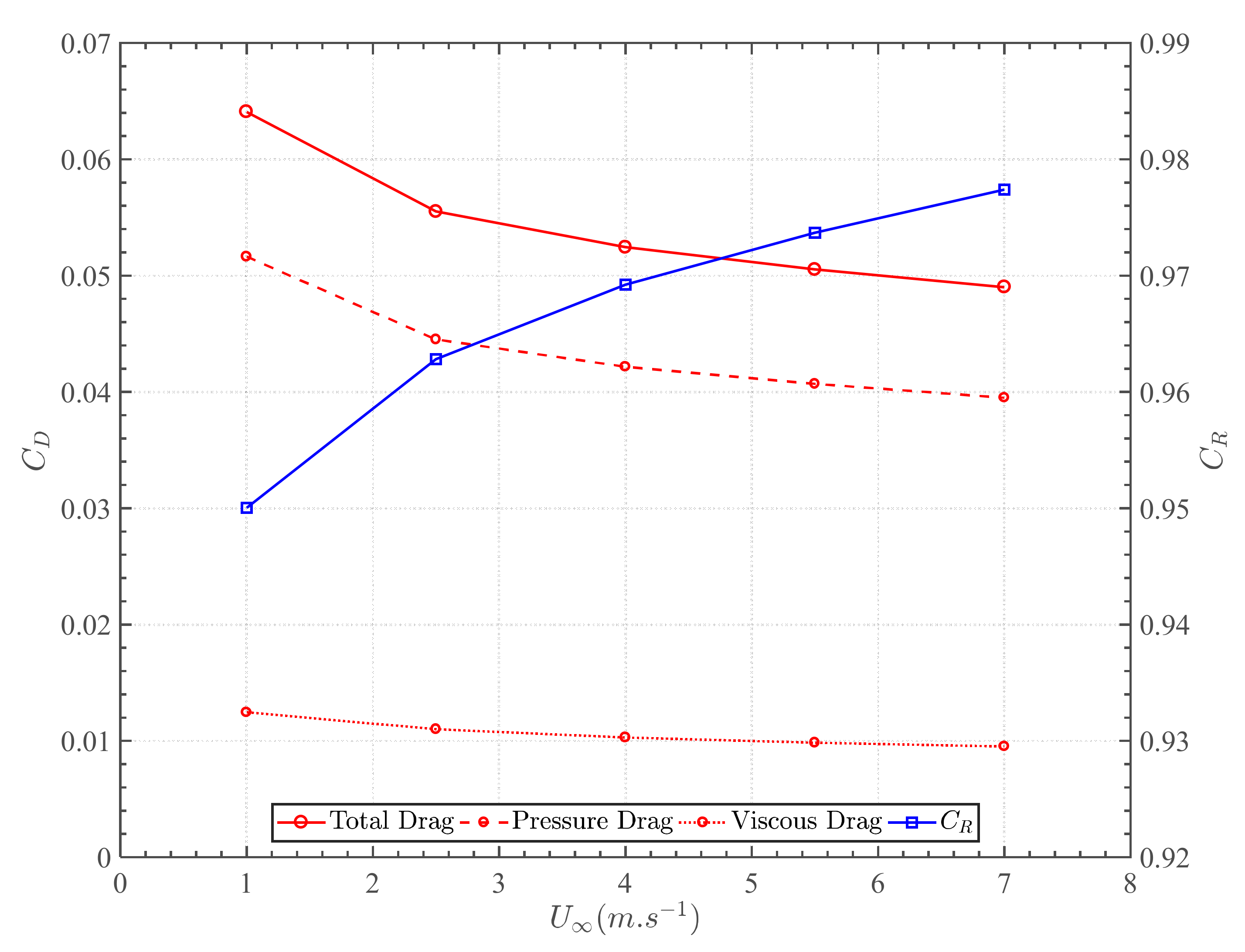
5.1. Drag Coefficient
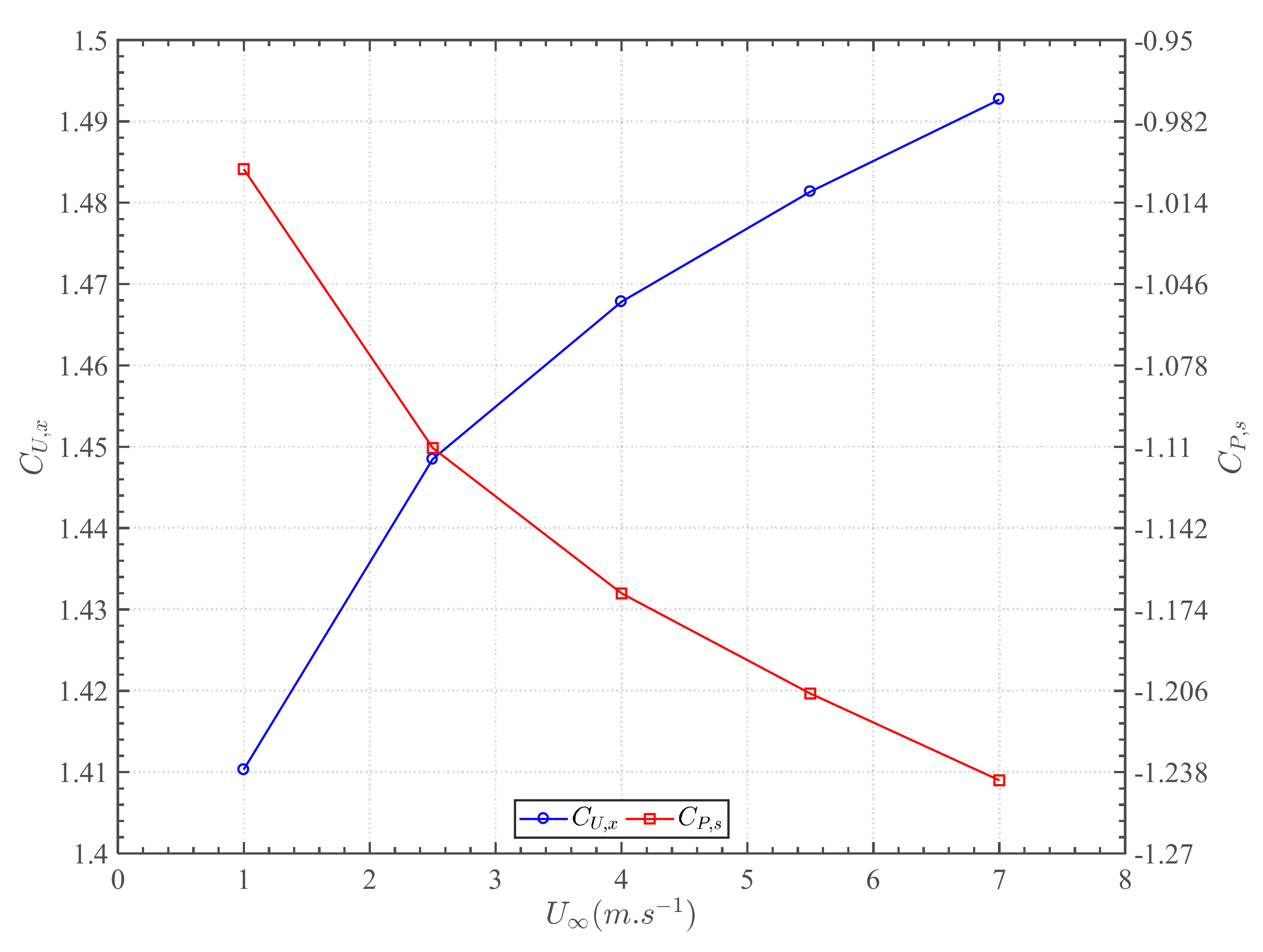
5.2. Axial Velocity and Static Pressure
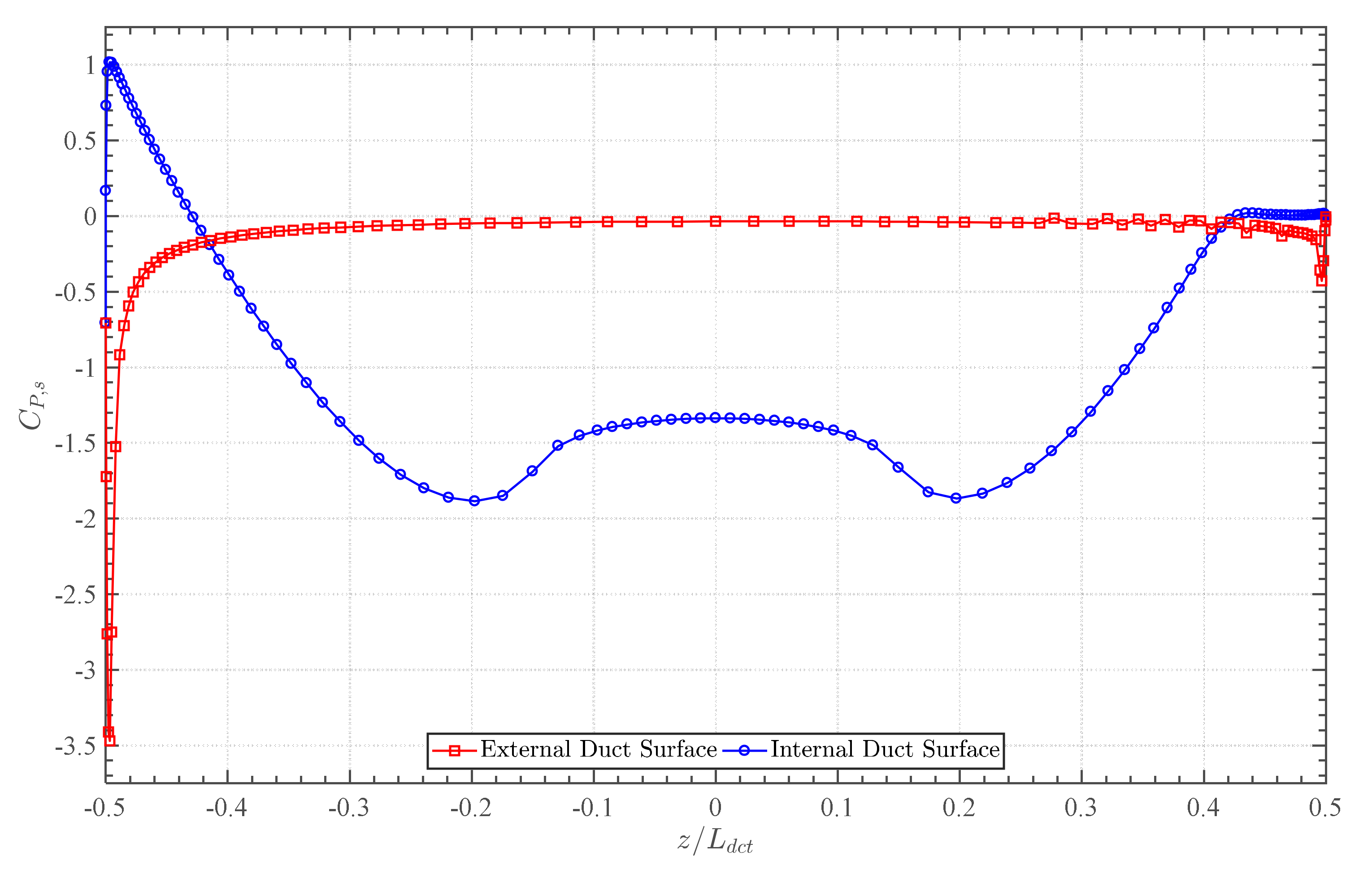
5.3. Duct Surface Static Pressure Coefficients
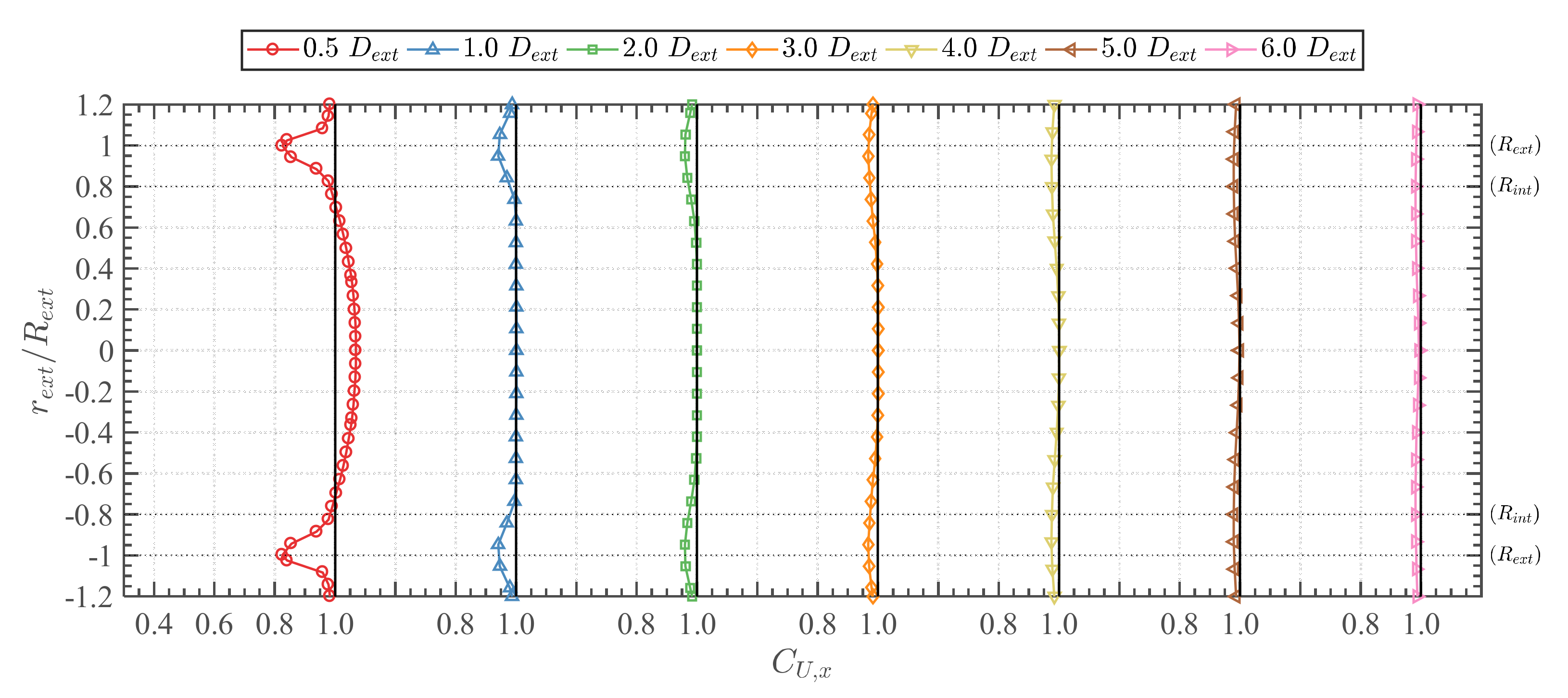
5.4. Wake Velocity Profiles
6. Vacant Duct Performance in Yawed Flow Conditions
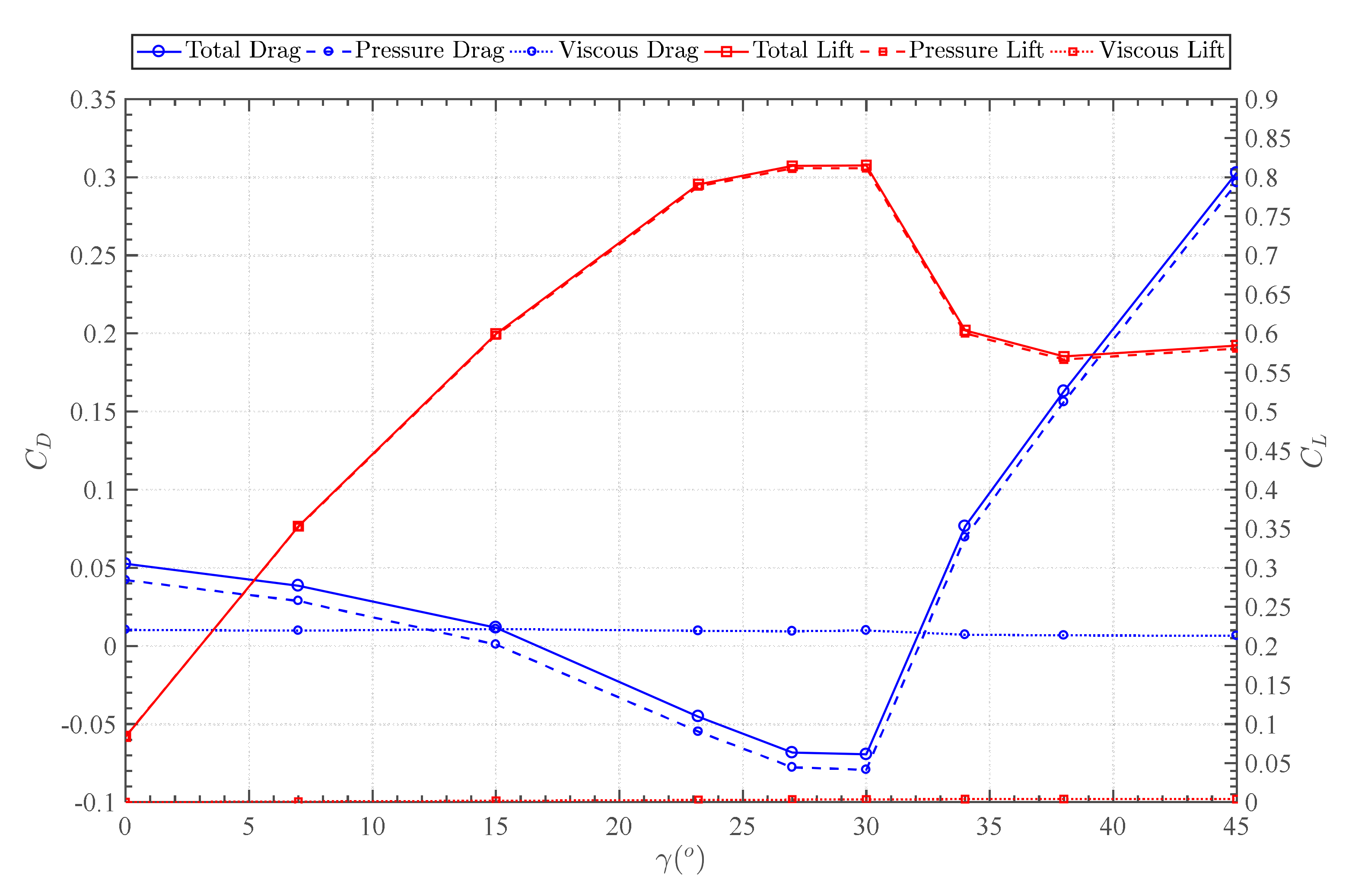
6.1. Drag and Lift Coefficients
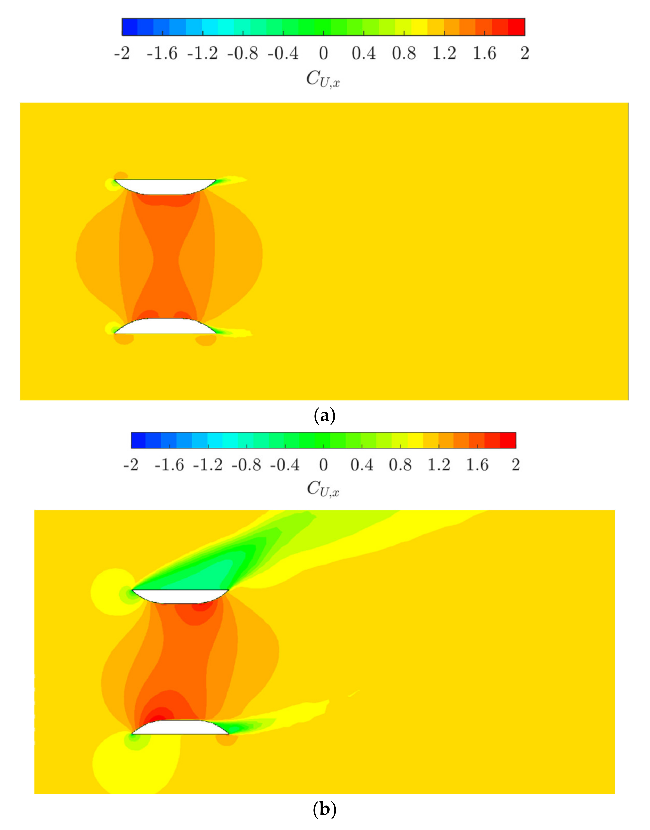
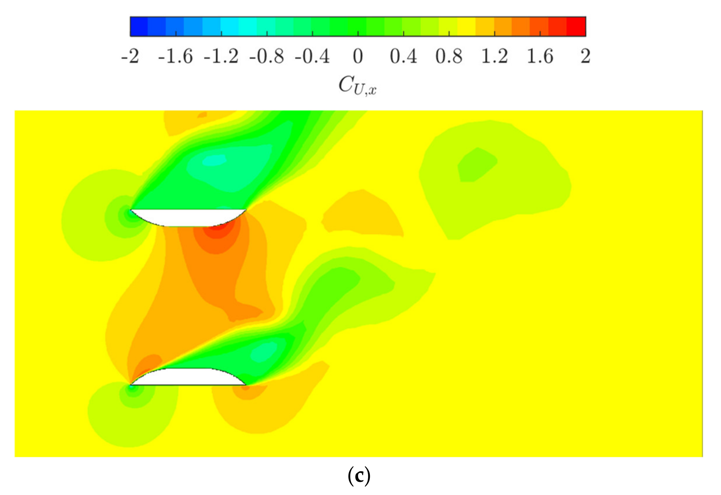
6.2. Axial Velocity and Static Pressure
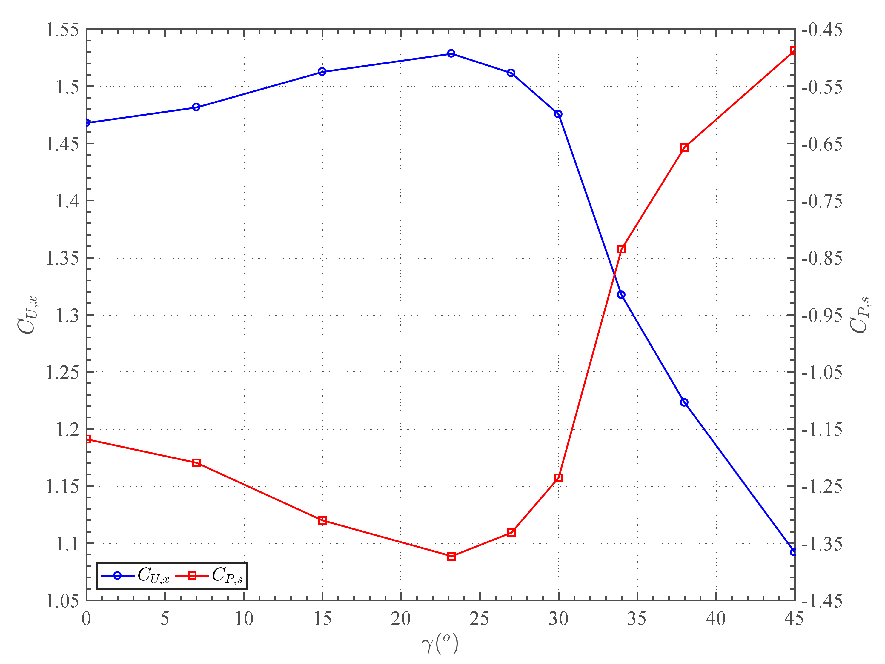
6.3. Duct Pressure Coefficients
7. Discussion
8. Conclusions
Author Contributions
Funding
Acknowledgments
Conflicts of Interest
Appendix A

References
- European Commission (Luxembourg: Office for Official Publications of the European Communities). A European Green Deal. Available online: https://ec.europa.eu/info/strategy/priorities-2019-2024/european-green-deal_en (accessed on 21 December 2020).
- Rourke, F.O.; Boyle, F.; Reynolds, A. Tidal energy update 2009. Appl. Energy 2010, 87, 398–409. [Google Scholar] [CrossRef]
- European Marine Energy Centre (EMEC) Ltd. Tidal Clients. Available online: http://tidalenergy.net.au/index-subpage-2.html (accessed on 2 February 2014).
- Goundar, J.N.; Ahmed, M.R. Design of a horizontal axis tidal current turbine. Appl. Energy 2013, 111, 161–174. [Google Scholar] [CrossRef]
- Kogan, F.A.; Seginer, A.T.A.E. Rep. No. 32A: Final Report on Shroud Design: Tech. Rep.; Department of Aeronautical Engineering, Technion-Israel Institute of Technology: Haifa, Israel, 1963. [Google Scholar]
- Bloomberg, L.P. OpenHydro Group Ltd. Available online: https://www.bloomberg.com/profile/company/4074464Z:ID2018 (accessed on 24 December 2020).
- OpenHydro Group Ltd. Projects. Available online: http://www.openhydro.com/Projects (accessed on 13 August 2017).
- The Canadian Press. Cape Sharp Tidal Turbine in Bay of Fundy Now Being Monitored Remotely. Available online: https://www.cbc.ca/news/canada/nova-scotia/cape-sharp-tidal-turbine-remote-monitoring-environment-1.4814069 (accessed on 15 September 2018).
- Ohya, Y.; Karasudani, T.; Sakurai, A.; Abe, K.; Inoue, M. Development of a shrouded wind turbine with a flanged diffuser. J. Wind Eng. Ind. Aerodyn. 2008, 96, 524–539. [Google Scholar] [CrossRef]
- Masukume, P.; Makaka, G.; Tinarwo, D. Optimum Geometrical Shape Parameters for Conical Diffusers in Ducted Wind Turbines. Int. J. Energy Power Eng. 2016, 5, 177–181. [Google Scholar]
- Masukume, P.-M.; Makaka, G.; Mukumba, P. Optimization of the Power Output of a Bare Wind Turbine by the Use of a Plain Conical Diffuser. Sustainability 2018, 10, 2647. [Google Scholar] [CrossRef]
- Setoguchi, T.; Shiomi, N.; Kaneko, K. Development of two-way diffuser for fluid energy conversion system. Renew. Energy 2004, 29, 1757–1771. [Google Scholar] [CrossRef]
- Cresswell, N.W.; Ingram, G.; Dominy, R. The impact of diffuser augmentation on a tidal stream turbine. Ocean Eng. 2015, 108, 155–163. [Google Scholar] [CrossRef]
- Kardous, D.M.; Chaker, R.; Aloui, F.; Nasrallah, S.B. On the dependence of an empty flanged diffuser performance on flange height: Numerical simulations and PIV visualizations. Renew. Energy 2013, 56, 123–128. [Google Scholar] [CrossRef]
- Kannan, T.S.; Mutasher, S.A.; Lau, Y.K. Design and flow velocity simulation of diffuser augmented wind turbine using CFD. J. Eng. Sci. Technol. 2013, 8, 372–384. [Google Scholar]
- Mansour, K.; Meskinkhoda, P. Computational analysis of flow fields around flanged diffusers. J. Wind Eng. Ind. Aerodyn. 2014, 124, 109–120. [Google Scholar] [CrossRef]
- Khamlaj, T.A.; Rumpfkeil, M.P. Analysis and optimization of ducted wind turbines. Energy 2018, 162, 1234–1252. [Google Scholar] [CrossRef]
- Kesby, J.E.; Bradney, D.R.; Clausen, P.D. Determining diffuser augmented wind turbine performance using a combined CFD/BEM method. J. Phys. Conf. Ser. 2016, 753, 10736–10774. [Google Scholar] [CrossRef]
- El-Zahaby, A.M.; Kabeel, A.; Elsayed, S.; Obiaa, M. CFD analysis of flow fields for shrouded wind turbine’s diffuser model with different flange angles. Alex. Eng. J. 2017, 56, 171–179. [Google Scholar] [CrossRef]
- Tampier, G.; Troncoso, C.; Zilic, F. Numerical analysis of a diffuser-augmented hydrokinetic turbine. Ocean Eng. 2017, 145, 138–147. [Google Scholar] [CrossRef]
- Borg, M.G.; Xiao, Q.; Allsop, S.; Incecik, A.; Peyrard, C. A numerical performance analysis of a ducted, high-solidity tidal turbine. Renew. Energy 2020, 159, 663–682. [Google Scholar] [CrossRef]
- Wilcox, D.C. Turbulence Modeling for CFD, 3rd ed.; DCW Industries, Inc.: San Diego, CA, USA, 2006. [Google Scholar]
- Neill, S.P.; Jordan, J.R.; Couch, S.J. Impact of tidal energy converter (TEC) arrays on the dynamics of headland sand banks. Renew. Energy 2012, 37, 387–397. [Google Scholar] [CrossRef]
- Bahaj, A.; Myers, L. Analytical estimates of the energy yield potential from the Alderney Race (Channel Islands) using marine current energy converters. Renew. Energy 2004, 29, 1931–1945. [Google Scholar] [CrossRef]
- Pham, C.T.; Martin, V.A. Tidal current turbine demonstration farm in Paimpol-Brehat (Brittany): Tidal characterisation and energy yield evaluation with TELEMAC. In Proceedings of the 8th European Wave and Tidal Energy Conference, Uppsala, Sweden, 7–8 September 2009. [Google Scholar]
- Pham, C.; Pinte, K. Paimpol-Bréhat tidal turbine demonstration farm (brittany): Optimisation of the layout, wake effects and energy yield evaluation using TELEMAC. In Proceedings of the 3rd International Conference on Ocean Energy, Bilbao, Spain, 6–7 October 2010. [Google Scholar]
- Mason-Jones, A.; O’Doherty, D.M.; Morris, C.E.; O’Doherty, T.; Byrne, C.B.; Prickett, P.W.; Grosvenor, R.I.; Owen, I.; Tedds, S.; Poole, R.J. Non-Dimensional Scaling of Tidal Stream Turbines. Energy 2012, 44, 820–829. [Google Scholar] [CrossRef]
- Resistance Committee of the 28th ITTC. Uncertainty Analysis in CFD Verification and Validation, Methodology and Procedures; Technical Report; ITTC: Zürich, Switzerland, 2017. [Google Scholar]
- Mycek, P.; Gaurier, B.; Germain, G.; Pinon, G.; Rivoalen, E. Experimental study of the turbulence intensity effects on marine current turbines behaviour. Part I: One single turbine. Renew. Energy 2014, 66, 729–746. [Google Scholar] [CrossRef]


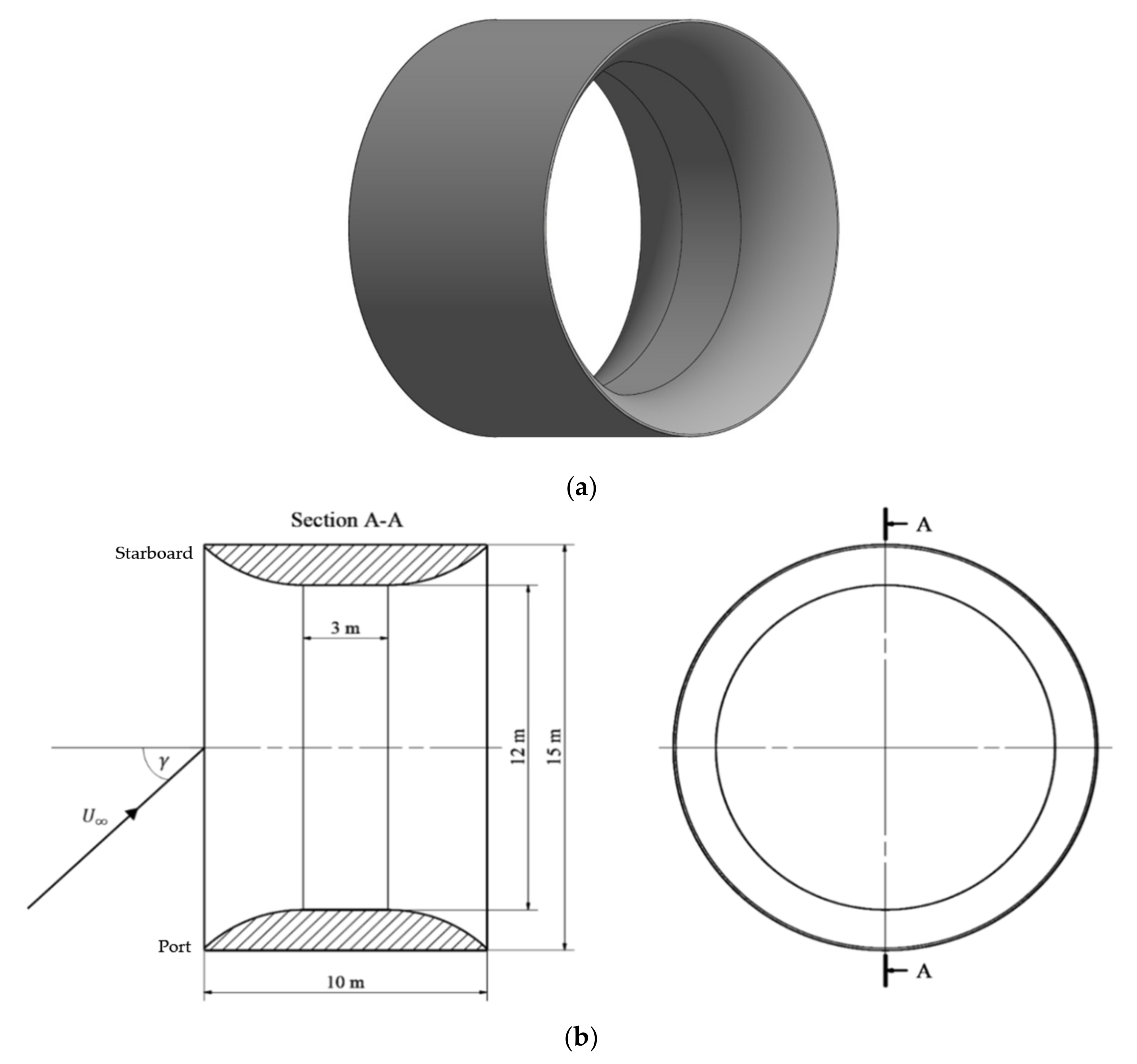
| Description | Value |
|---|---|
| Duct external diameter () | 15 m |
| Duct internal radius () | 12 m |
| Duct length () | 10 m |
| Reynolds number () | [0.149 − 1.046] × |
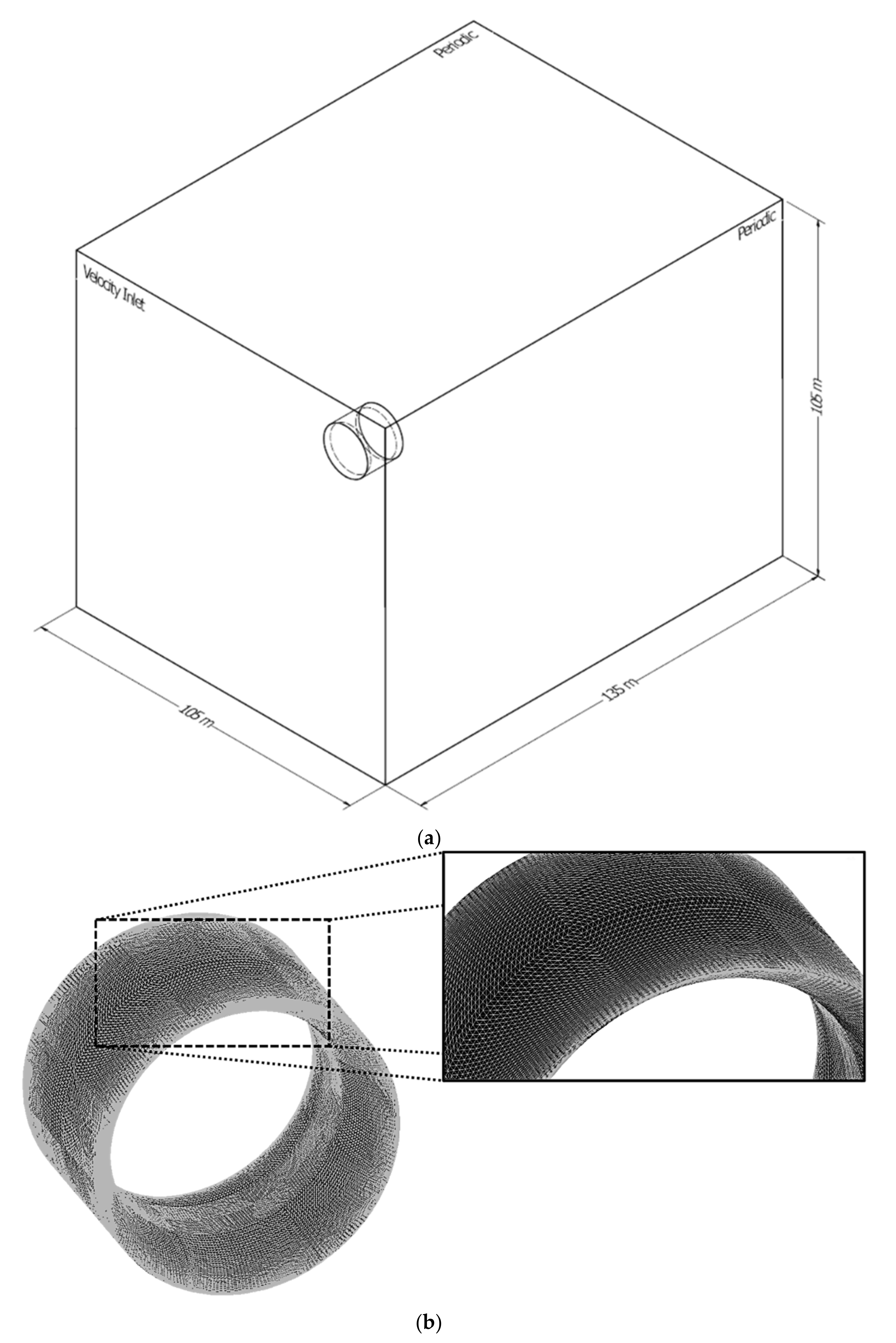
| Description | Aligned Flow | Yawed Flow |
|---|---|---|
| Free-stream velocity () | 1 m.s−1, 2.5 m.s−1, 4 m.s−1, 5.5 m.s−1, 7 m.s−1 | 4 m.s−1 |
| Yaw bearing () | 0 | 0, 7, 15, 23.2, 27, 30, 38, 45 |
| n | Cell Number | Cell Number Ratio | S | ε | ψ |
|---|---|---|---|---|---|
| 3 | 6,533,300 | 1.247 | 1.493 | 0.0062 | 0.569 |
| 2 | 5,240,241 | 1.277 | 1.487 | 0.0109 | |
| 1 | 4,103,210 | 1.476 |
Publisher’s Note: MDPI stays neutral with regard to jurisdictional claims in published maps and institutional affiliations. |
© 2021 by the authors. Licensee MDPI, Basel, Switzerland. This article is an open access article distributed under the terms and conditions of the Creative Commons Attribution (CC BY) license (http://creativecommons.org/licenses/by/4.0/).
Share and Cite
Borg, M.G.; Xiao, Q.; Allsop, S.; Incecik, A.; Peyrard, C. A Numerical Swallowing-Capacity Analysis of a Vacant, Cylindrical, Bi-Directional Tidal Turbine Duct in Aligned & Yawed Flow Conditions. J. Mar. Sci. Eng. 2021, 9, 182. https://doi.org/10.3390/jmse9020182
Borg MG, Xiao Q, Allsop S, Incecik A, Peyrard C. A Numerical Swallowing-Capacity Analysis of a Vacant, Cylindrical, Bi-Directional Tidal Turbine Duct in Aligned & Yawed Flow Conditions. Journal of Marine Science and Engineering. 2021; 9(2):182. https://doi.org/10.3390/jmse9020182
Chicago/Turabian StyleBorg, Mitchell G., Qing Xiao, Steven Allsop, Atilla Incecik, and Christophe Peyrard. 2021. "A Numerical Swallowing-Capacity Analysis of a Vacant, Cylindrical, Bi-Directional Tidal Turbine Duct in Aligned & Yawed Flow Conditions" Journal of Marine Science and Engineering 9, no. 2: 182. https://doi.org/10.3390/jmse9020182
APA StyleBorg, M. G., Xiao, Q., Allsop, S., Incecik, A., & Peyrard, C. (2021). A Numerical Swallowing-Capacity Analysis of a Vacant, Cylindrical, Bi-Directional Tidal Turbine Duct in Aligned & Yawed Flow Conditions. Journal of Marine Science and Engineering, 9(2), 182. https://doi.org/10.3390/jmse9020182