A Unifying Task Priority Approach for Autonomous Underwater Vehicles Integrating Homing and Docking Maneuvers

Abstract

This research proposes a unified guidance and control framework for Autonomous Underwater Vehicles (AUVs) based on the task priority control approach, incorporating various behaviors such as path following, terrain following, obstacle avoidance, as well as homing and docking to stationary and moving stations. The integration of homing and docking maneuvers into the task priority framework is thus a novel contribution of this paper. This integration allows, for example, to execute homing maneuvers close to uneven seafloor or obstacles, ensuring the safety of the AUV, as safety tasks can be given the highest priority. Furthermore, another contribution shown in the paper is that the proposed approach tackles a wide range of scenarios without ad hoc solutions. Indeed, the proposed approach is well suited for both the emerging trend of resident AUVs, which stay underwater for a long period inside garage stations, exiting to perform inspection and maintenance missions and homing back to them, and for AUVs that are required to dock to moving stations such as surface vehicles, or towed docking stations. The proposed techniques are studied in a simulation setting, taking into account the rich number of aforementioned scenarios.

1. Introduction

In the past couple of decades, we have seen a tremendous increase in the use of Autonomous Underwater Vehicles (AUVs) in a wide variety of applications ranging from sub-sea explorations to ocean research and development [1]. Some notable areas where AUVs are widely used [2] involve mapping, inspections, surveys, and military roles. Damages from incidents such as the Deepwater Horizon tragedy [3] could have considerably reduced if there was a possibility of using an AUV for inspecting the blowout preventer, riser, and surrounding seabed of the oil rig. Necessary precautions and safety measures could have been taken well in advance to reduce the impact of such mishaps. Now, AUVs have evolved to accomplish complex and highly demanding tasks such as search and rescue [4], underwater manipulation [5], homing, docking [6], etc. Apart from this, these underwater vehicles are required to autonomously carry out mission tasks that includes path following, terrain following, obstacle avoidance, and such. A growing trend [7] has been observed with a new class of vehicles named field resident AUV systems that carry out these tasks. Complementing the Remotely Operated Vehicles (ROVs) in the midterm [8,9], resident AUVs now hold a position as a completely unique class of underwater robotic systems merging the advances in technology and demand for new applications. The various components of such systems [10] additionally include a home base for docking when not performing the mission, and various power and communication facilities. In [11], the authors conducted a workshop that studied various applications of resident AUVs, focusing more on mid-water and seafloor observations. In [12], the authors discuss some capabilities of such systems by studying the Marlin Mk3 AUV by Lockheed Martin and Saab Seaeye’s Sabertooth AUV. The work in [13] is about the deployment of resident AUV Systems by Chevron for pipeline and facility inspection operations. FlatFish [14] is used to perform an on-demand close visual inspection on sub-sea structures within an oil and gas field. The work in [15] discusses the monitoring of underwater infrastructure using a resident AUV Tri-TON 2. Saipem has developed a resident AUV named Hydrone-R1 capable of carrying out light construction works and advanced inspections on sub-sea assets. In [16], the authors conduct a review of resident AUV systems, along with their application areas, capabilities, and challenges. Such class of AUVs are thus needed by the current industry, favoring a system that is capable of carrying out all tasks and operations autonomously, thus motivating the problem of autonomous mission capability, homing, and docking. Another increasing trend sees AUVs deployed from surface vessel or submarines, and requires them to home back autonomously. Retrieval of REMUS 100 AUV from an Autonomous Surface Vehicle (ASV) using a taut tether line is presented in [17], while docking of AUVs to a submarine is presented in [18]. The work in [19] discusses the launch, deployment, and recovery of AUVs from submarines via conventional torpedo tubes and via a hangar mounted to the submarine body. In [20], the authors present the recovery of AUVs from submarines by operating a taught wire for retrieval. Thus, autonomous deployment, homing, and docking are desirable features for AUVs. For long-term deployments, it is required to have these capabilities carried out without any intervention from any human operators. Having these autonomous capabilities could save time, and reduce human error and fatigue, even for systems such as ROVs or other tethered underwater or surface vehicles. It is thus interesting to study and find solutions in the autonomous capabilities of the vehicle that would encompass all behaviors that are needed right from dispatch till recovery, and also with a long-term vision of intervention capabilities [21,22].

Given the aforementioned trends, it is clear that there is a need to integrate into AUVs the capability to home into and be able to dock into a stationary or moving docking station, be it underwater such as submarines, a station on the seafloor, or on the surface such as a surface vehicle. The docking maneuver is usually performed in two phases: The first phase is a long-range homing that involves the identification of the homing signal from the docking system by the AUV to proceed in the general direction of the homing signal. As the AUV approaches closer to the docking station, the terminal docking phase is performed where the AUV proceeds further towards the docking system and attains the dock position. Recent trends denote that this homing and approach maneuver is performed largely by ad hoc controllers. In [23], the authors discuss a docking system designed for REMUS AUV that allows acoustic homing to the docking station. The work in [24] presents a docking assessment algorithm for assessing the feasibility of the desired path for docking of a torpedo-shaped AUV using depth tracking via neural network-generated paths, docking feasibility region analysis to provide a possibility region of successful docking, and docking success probability evaluation based on the probability of sensor data. A vision-based docking system [25] was developed for Starbug AUV where a target is detected using a fast pole detection algorithm based on Haar rectangular features and image rotations. In [26], the authors discuss an optical quadrant tracker method for terminal guidance of underwater vehicles to control the horizontal and vertical movements of the vehicle by appropriate proportional fin commands, thereby steering the vehicle. A vision-based localization for resident underwater vehicles, consisting of beacon lights attached to a tether management system, creating a unique light marker fixed at the target location for pose estimation, is discussed in [27]. Docking of intervention AUVs using sonar and video image processing algorithms accompanied with navigational data obtained from conventional sensors is explained in [28]. The work in [29] discusses the concept and testing of a bio-inspired electromagnetic homing guidance system developed for AUVs at close range to the dock, using a differential magnetometer system fitted with magnetic field sensors at the forward and aft of the AUV for detecting the dipole magnetic field of fixed frequency and power generated from the dock.

Furthermore, just like ASVs, AUVs needs to be docked to surface docking stations such as piers, mother ships, etc. for system inspection or safe retrieval. Autonomous docking of an AUV to surface docking stations can be assumed as a special case of autonomous docking of ASV. In [30], the authors discuss docking of an ASV using linear- and circular-based vector field guidance methods to overcome the motion constraints in performing docking to certain regions where it is difficult to dock without collision with structures such as pier walls. A combination of circular and linear vector fields are suggested to drive the vehicle out from the collision region. However, if the vehicle starts too close to the structures, there is a chance of collision as the vehicle might perform some tight maneuvers. Coming to moving docking stations, the authors of [31] integrate no-fly zones with virtual obstacles into the navigation function for avoiding collisions while trying to dock from the stern direction into a docking station hoisted on top of a submarine. A method of recovery for AUVs using a visual docking approach is discussed in [32] where the terminal guidance is performed via two cameras that help in estimating the position of a moving docking station. The position and heading of the AUV is corrected before controlling its vertical movement to finally dock to the docking platform. In their work, the authors consider the moving dock to be in the mid-water column (i.e., in the free space). However, if the dock is close to the seafloor, the terrain may not be smooth. As the vehicle approaches for docking in such scenarios, it could have unwanted collisions with the seafloor while attempting the docking maneuver. The work in [33] discusses the docking of ASVs into a large mother ship by placing a virtual target to a point positioned at the projection of the ASV position onto a safety circle surrounding the mother ship. This virtual target point can move along the safety circle until its bearing matches up with that of the desired docking point. Once the ASV matches its position and velocity with this virtual target point, the target point starts reducing its distance from the dock by translating, until it becomes equal to that of the docking point. However, the fully translation maneuver presented in the homing and docking stages will be difficult to achieve due to the drag, presence of water currents, and high energy requirements.

Coming further, a robust guidance system can be identified as a core and crucial component for ensuring successful autonomous operations. For executing certain maneuvers close to the seafloor or near structures, underwater vehicles would require sophisticated control systems to guide the vehicle around obstacles, maintain a certain altitude or depth, all in the possible presence of ocean currents. Another interesting fact is that the previously discussed techniques take only a specific type of behavior into account. Those techniques do not incorporate diverse behaviors, ranging from the execution of the main tasks of the mission (e.g., surveying an area, structure, etc.), to homing and docking at the end of the mission. For systems such as industrial and residential applications where the automatic procedures are important, it will be desirable to have a fully fledged control framework to solve all different control problems. Due to this increase in the capabilities assigned to the vehicle, there is a transition observed with the use of a unified guidance and control framework. The task priority framework [34,35,36,37,38] is flexible and can accommodate various tasks and operations that are required, favoring a priority-based systematic execution of tasks. Not only does it provide a unified approach, but also a systematic control that will, if required, take into account additional features such as physical/operational constraints of the vehicle (e.g., vehicle under-actuation), safety limits (e.g., maintaining a safe distance from dock to avoid collision), constraints in approach (e.g., docking from stern), and energy expenditure (e.g., minimize drag by exploiting translation only when necessary), to name but a few. A priority-based control to integrate inequality control objectives and task transitions is presented in [39], displaying how inequality control objectives could be well defined within the task priority framework without causing any discontinuities. This was further expanded in the MARIS, DexROV, and ROBUST projects [40,41,42,43]. The work in [44] shows the capabilities of the task priority framework in the cooperative control of multiple underwater manipulators where a cooperative transportation scenario is considered (the same strategy has been demonstrated with ground mobile manipulators showing experimental results in [45]). Inspired from these literatures, a task priority control framework is used as the control framework for our research. Various tasks are defined in the framework where they are achieved in the order of priority. Thanks to the flexibility in incorporating various tasks, it is now easier to expand the capabilities of our controller.

This paper contributes by focusing on a general control strategy, proposing a unified AUV guidance and control based on the task priority control framework and improving the previously discussed literature as explained further. We take into account the various behaviors of underwater vehicles and implement all of these features within the common unified framework of task priority based control. The outline of the contributions are as follows. Tasks are incorporated that support various type of missions thereby generating complex behaviors. The parking maneuver and docking maneuver are cast as particular tasks and are integrated with the safety tasks into one particular structured behavior of the system, improving over the state of the art. The work in [30] is improved by using velocity field control technique [46,47] that produces a curvilinear trajectory for approaching in the desired orientation well in advance, and using a concept similar to the virtual obstacles proposed in [31] for avoiding any collisions while approaching or performing tight maneuvers close to the docking station. Compared to the work in [32], we additionally consider a case in which the docking station is close to the seafloor where the terrain may not be smooth. We execute the final homing and docking maneuver by following the seafloor, also maintaining a safe altitude. The work in [33] is improved by aligning the vehicle heading with the system velocity for reducing drag and high energy requirements during the homing and approach stages. The advantages of these contributions are that all these challenging conditions along with mission execution, homing and parking are integrated into the same task priority framework. The proposed approach also allows docking from any initial condition of the vehicle to a stationary or moving docking station traveling in free space, close to the seafloor or on the surface. Additionally, pitch limitation is also implemented to avoid the vehicle from reaching pitches above its permissible limits.

With the aim of showing the aforementioned contributions, the remaining paper is structured as follows. Section 2 introduces the fundamentals of the task priority framework. The task priority approach integrating homing and docking maneuvers, along with path following, terrain following, depth control, altitude control, and obstacle avoidance for various mission scenarios are detailed in Section 3. Simulation results are discussed in Section 4 along with plots displaying the various behaviors of the system. Section 5 concludes the paper.

2. General Notations and Model Definition

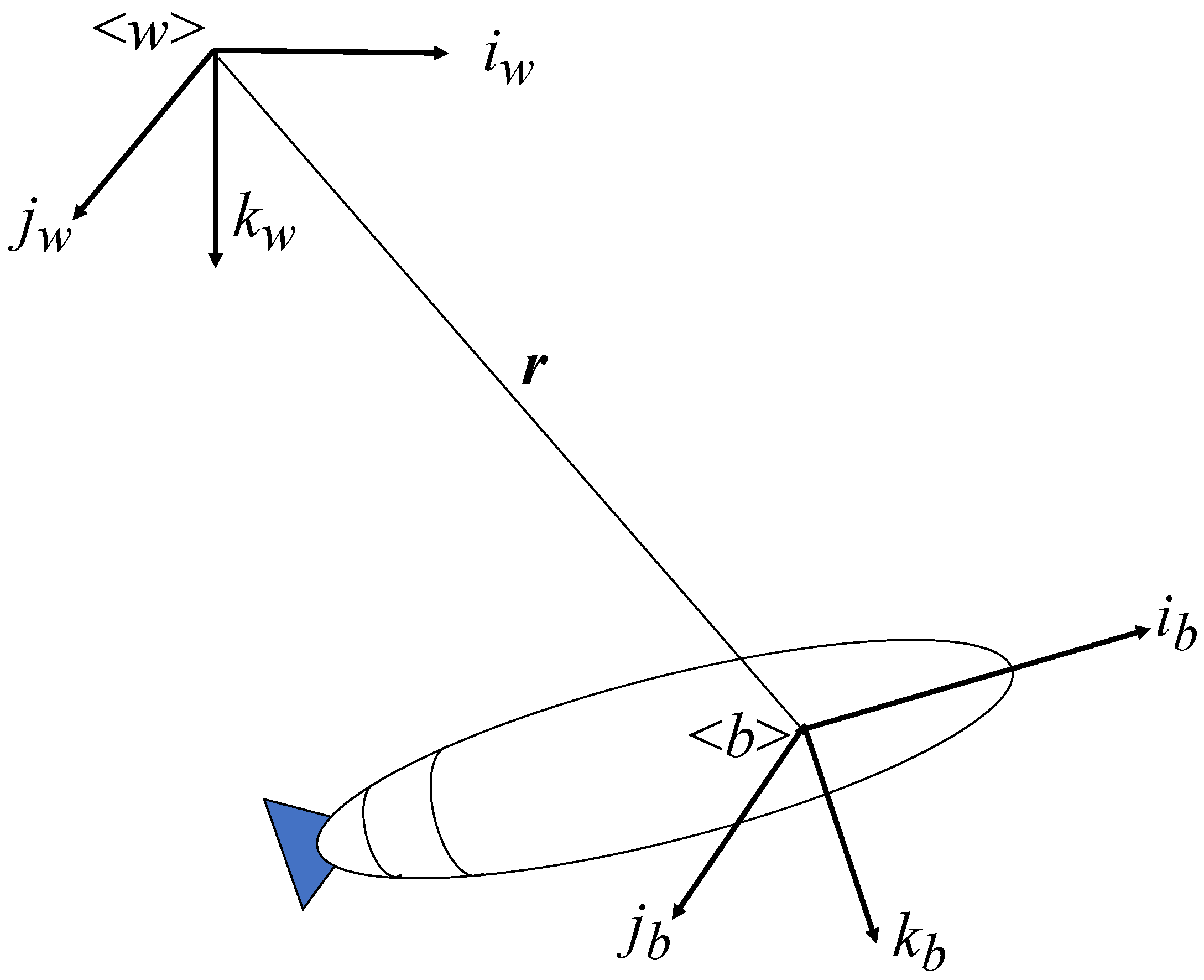
2.1. Frames and Transformations

To determine the position, orientation, and velocity of the vehicle, the paper uses two reference frames: a world-fixed reference frame $\langle w\rangle$ and a body fixed reference frame $\langle b\rangle$ as shown in Figure 1. The $\langle w\rangle$ frame has its x axis pointing to the North, the y axis pointing to the East, and the z axis pointing to the center of the Earth. The unit vectors representing each directions in $\langle w\rangle$ are ${\mathit{i}}_w$, ${\mathit{j}}_w$ and ${\mathit{k}}_w$, respectively. The $\langle b\rangle$ frame relates to the vehicle with its x axis pointing to the forward direction, the y axis to the right direction, and the z axis points vertically down. The unit vectors representing each directions in $\langle b\rangle$ are ${\mathit{i}}_b$, ${\mathit{j}}_b$ and ${\mathit{k}}_b$, respectively. Both these frames are related by the Euler angles yaw($\psi$), pitch($\theta$), and roll($\varphi$). Let ${\mathit{\eta }}_1={[x,y,z]}^{\top }$ represent the position vector of origin of frame $\langle b\rangle$ w.r.t. $\langle w\rangle$ and ${}^w{\mathit{R}}_b$ or simply $\mathit{R}$ represents the orientation matrix of $\langle b\rangle$ frame w.r.t. $\langle w\rangle$ frame as

$${}^w{\mathit{R}}_b=\left[\begin{array}{ccc}c\psi c\theta & -s\psi c\varphi +c\psi s\theta s\varphi & s\psi s\theta +c\psi c\varphi s\theta \\ s\psi c\theta & c\psi c\varphi +s\varphi s\theta s\psi & -c\psi s\varphi +s\theta s\psi c\varphi \\ -s\theta & c\theta s\varphi & c\theta c\varphi \end{array}\right],$$

(1)

where c and s denote the cosine and sine values of the respective Euler angles, respectively. The transformation matrix of $\langle b\rangle$ frame w.r.t. $\langle w\rangle$ frame is thus given by ${}^w{\mathit{T}}_b=\left[\begin{array}{cc}{}^w{\mathit{R}}_b& {\mathit{\eta }}_1\\ 0& 1\end{array}\right]$.

2.2. AUV Kinematic and Dynamic Model

This section discusses the general kinematic and dynamic model of the vehicle presented in the paper. We consider a class of torpedo-shaped vehicles that can translate, and it has 5 actuated degrees of freedom which are along the surge, sway, heave, pitch, and yaw directions. The notations used in this paper to describe rigid-body dynamics follow the conventions of the Society of Naval Architects and Marine Engineers (SNAME) presented in [48]. In the state space representation, $\mathit{\eta }=[{{\mathit{\eta }}_{\mathbf{1}}}^{\top }$${{\mathit{\eta }}_{\mathbf{2}}}^{\top }{]}^{\top }\in {\mathbb{R}}^{6\times 1}$ represents the vehicle position vector ${[x,y,z,\varphi ,\theta ,\psi ]}^{\top }$ in $\langle w\rangle$ frame. ${}^b\mathit{\nu }={\left[{}^b{\mathit{v}}^{\top }{}^b{\mathit{\omega }}_{b/w}^{\top }\right]}^{\top }\in {\mathbb{R}}^{6\times 1}$ represents the generalized velocities expressed in $\langle b\rangle$, where ${}^b\mathit{v}={[u,v,w]}^{\top }\in {\mathbb{R}}^{3\times 1}$ is the absolute linear velocity and ${}^b{\mathit{\omega }}_{b/w}={[p,q,r]}^{\top }\in {\mathbb{R}}^{3\times 1}$ is the angular velocity of the $\langle b\rangle$ w.r.t. $\langle w\rangle$ expressed in $\langle b\rangle$.

2.2.1. Kinematic Model

The kinematic model links the derivative of the absolute position and the yaw–pitch–roll Euler derivatives to the relative velocity of the vehicle w.r.t. the water, the ocean current velocity and the angular velocity of the vehicle using the following relationship,

$$\dot{\mathit{\eta }}=\left[\begin{array}{c}\mathit{R}\left({\mathit{\eta }}_{\mathbf{2}}\right){}^b{\mathit{v}}_{\mathit{r}}\\ {\mathit{J}}_{\mathit{e}}\left({\mathit{\eta }}_{\mathbf{2}}\right){}^b{\mathit{\omega }}_{b/w}\end{array}\right]+\left[\begin{array}{c}{}^w{\mathit{v}}_{\mathit{c}}\\ 0\end{array}\right],$$

(2)

where $\dot{\mathit{\eta }}={[\dot{x},\dot{y},\dot{z},\dot{\varphi },\dot{\theta },\dot{\psi }]}^{\top }$, ${}^b{\mathit{v}}_{\mathit{r}}\in {\mathbb{R}}^{3\times 1}$ is the relative linear velocity vector (w.r.t. the water), ${}^w{\mathit{v}}_{\mathit{c}}\in {\mathbb{R}}^{3\times 1}$ is the linear velocity of ocean current (assuming the current to be irrotational and ${\dot{\mathit{v}}}_c=0$). ${\mathit{J}}_{\mathit{e}}\left({\mathit{\eta }}_{\mathbf{2}}\right)$ is the Jacobian connecting the body angular velocities ${}^b{\mathit{w}}_{b/w}$ to the y-p-r Euler rates ${\dot{\mathit{\eta }}}_2$, given as

$${\mathit{J}}_{\mathit{e}}\left({\mathit{\eta }}_{\mathbf{2}}\right)=\left[\begin{array}{ccc}1& s\varphi t\theta & c\varphi t\theta \\ 0& c\varphi & -s\varphi \\ 0& s\varphi /c\theta & c\varphi /c\theta \end{array}\right],$$

(3)

where c, s and t denote the cosine, sine and tangent values of the respective Euler angles.

2.2.2. Dynamic Model

The dynamic model of the vehicle is based on the general Fossen model for underwater vehicles [49,50,51]. The Newton--Euler dynamic equations of motion are given by

$${}^b{\mathit{\nu }}_r={}^b\mathit{\nu }-{}^b{\mathit{\nu }}_c,$$

(4)

$$\left({\mathit{M}}_{rb}+{\mathit{M}}_A\right){}^b{\dot{\mathit{\nu }}}_r+\left({\mathit{C}}_{rb}\left({}^b{\mathit{\nu }}_r\right)+{\mathit{C}}_A\left({}^b{\mathit{\nu }}_r\right)\right){}^b{\mathit{\nu }}_r+\mathit{D}\left({}^b{\mathit{\nu }}_r\right){}^b{\mathit{\nu }}_r+{}^b{\mathit{\tau }}_{rf}={}^b{\mathit{\tau }}_v+{}^b{\mathit{\tau }}_L+{}^b{\mathit{\tau }}_E,$$

(5)

where ${}^b{\mathit{\nu }}_r\in {\mathbb{R}}^{6\times 1}$ is the generalized vector of body relative velocities, ${}^b{\mathit{\nu }}_c\in {\mathbb{R}}^{6\times 1}$ is the generalized vector of ocean current velocity, $\left({\mathit{M}}_{rb}+{\mathit{M}}_A\right)$ is the system inertia matrix (including added mass), $\left({\mathit{C}}_{rb}\left({}^b{\mathit{\nu }}_r\right)+{\mathit{C}}_A\left({}^b{\mathit{\nu }}_r\right)\right)$ represents the Coriolis and centripetal matrix (including added mass), $\mathit{D}\left({}^b{\mathit{\nu }}_r\right)$ is the drag matrix, ${}^b{\mathit{\tau }}_{rf}$ is the generalized vector of restoring forces (gravitational and buoyancy), ${}^b{\mathit{\tau }}_v$ represents the generalized vector of propulsion forces, ${}^b{\mathit{\tau }}_L$ is the generalized vector of lifting forces, and ${}^b{\mathit{\tau }}_E$ is the generalized vector of environment forces on a rigid body. As the fluid flow is expected to be traversal/longitudinal w.r.t. the length of the vehicle during typical operating conditions such as hovering or forward motion characterized by slow velocities and accelerations (thus small angles of attack), the lift forces and moments are expected to be negligible w.r.t. drag forces and moments and can be neglected. The drag matrix $\mathit{D}\left({}^b{\mathit{\nu }}_r\right)$ is modeled as the sum of the linear and quadratic damping terms with diagonal structure as

$$\mathit{D}\left({}^b{\mathit{\nu }}_r\right)=\left({\mathit{D}}_I+{\mathit{D}}_q\left({}^b{\mathit{\nu }}_r\right)\right),$$

(6)

The generalized vector of propulsion forces produced by the thrusters, is given by

$${}^b{\mathit{\tau }}_{\mathit{v}}=\mathit{B}\left({}^b{\mathit{\nu }}_r\right)\mathit{u},$$

(7)

where $\mathit{u}\in {\mathbb{R}}^{5\times 1}$ is the vector of control inputs in which each component is the force produced by the respective thruster and $\mathit{B}$ is the control allocation or mapping matrix that allows computing the resulting body wrench ${}^b{\mathit{\tau }}_v$, given a certain $\mathit{u}$. The relation between the force of a given thruster and its velocity is highly nonlinear and depends on the thruster characteristics, thruster motor velocity, and the fluid velocity passing through the thruster. Note that the specific model parameters will be revisited in the Section 4.1 where we will discuss more on the vehicle at hand.

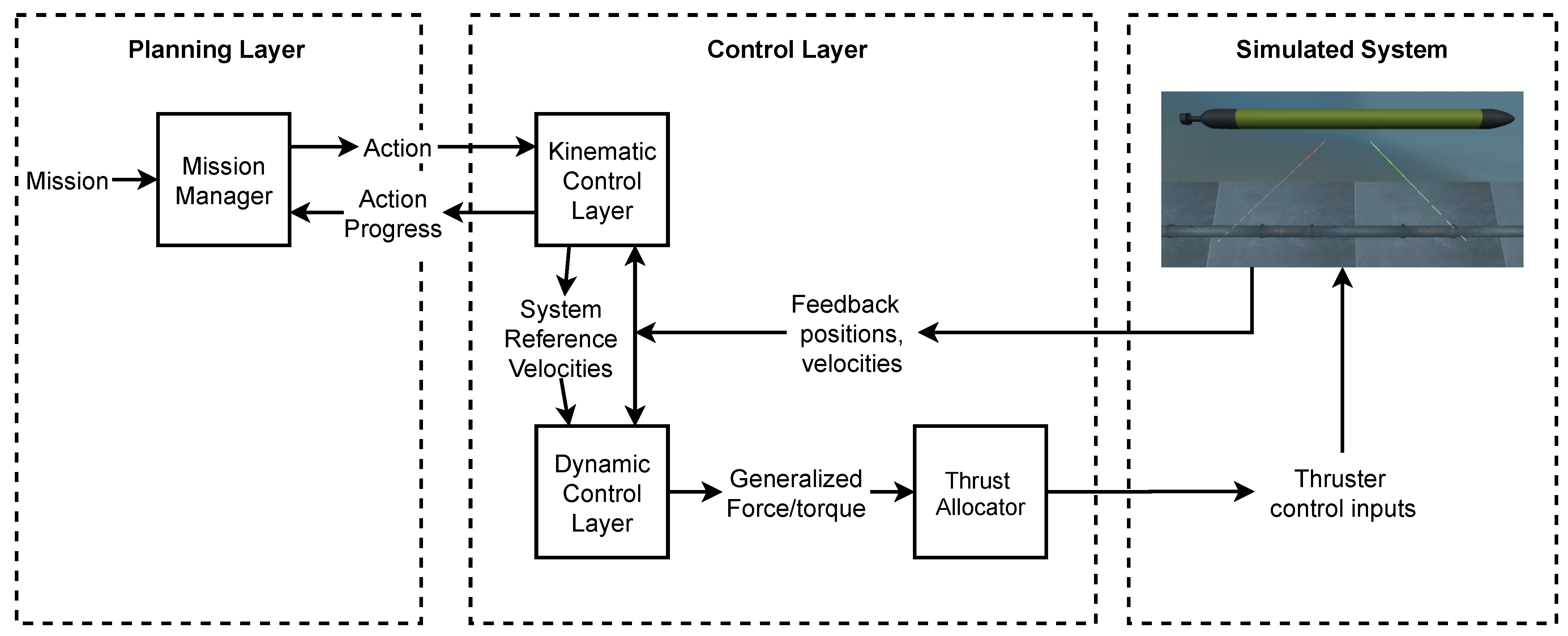
3. Control Architecture

A general schematic of the control architecture is provided in Figure 2 and is composed by three layers: the Planning Layer, the Control Layer, and the Simulated System. The force that each thruster must exert, which is an input to the Simulated System, is found using the thruster allocation mechanism that maps the desired wrench on the body to the forces that need to be generated by each of the thrusters. Such a desired wrench is the output of the Dynamic Control Layer (DCL), which tracks the desired system velocities. The Kinematic Control Layer (KCL) encompasses the definition of the control tasks, which are the basic building block of the architecture. Within the KCL, basic tasks are arranged into task hierarchies with priorities that constitute the control actions. The KCL receives the action to be executed from the Planning Layer, and it exploits the proposed task priority framework to find out the desired system velocity to accomplish it. The Planning Layer contains the mission manager that supervises and manages the execution of the current mission. It also addresses conflicting tasks by sequencing different actions or by providing a new set of parameters, thus providing an alternate solution. We recall that in the scope of this paper, we will focus on the properties of the KCL without going into details of DCL and Planning Layer.

3.1. Task Priority Framework and Definitions

The KCL implements the task priority framework that is presented in [37]. In this task priority framework approach, objectives define a specific condition that needs to be satisfied. Consider a position dependent scalar variable $x\left(\mathit{\eta }\right)$, then an equality control objective should satisfy $x\left(\mathit{\eta }\right)=x_0$ as $t\to \infty$ and, an inequality control objective should satisfy $x\left(\mathit{\eta }\right)\le x_{max}$ or $x\left(\mathit{\eta }\right)\ge x_{min}$ as $t\to \infty$. To satisfy this control objective, the time derivative of the variable $x\left(\mathit{\eta }\right)$ should allow it to converge to the desired region or value. For ensuring a closed-loop convergence, a desired feedback reference rate $\dot{\overline{x}}$ is defined as [42]

$$\dot{\overline{x}}\left(x\right)\triangleq \kappa (x^{*}-x),\kappa >0,$$

(8)

where $x^{*}$ denotes an arbitrary point that satisfies the objective. $\kappa$ is a positive gain proportional to the desired rate of convergence of the variable in consideration. The Jacobian relationship linking the variables x to the system velocity vector $\dot{\mathit{\nu }}$ is

$$\dot{x}={\mathit{g}}^{\top }\dot{\mathit{\nu }},$$

(9)

where the vector $\mathit{g}\in {\mathbb{R}}^n$ denotes the Jacobian for the task. A task will track the desired feedback reference rate $\dot{\overline{x}}$, to drive the associated variable $x\left(\mathit{\eta }\right)$ towards its corresponding objective. Thus, the task will ensure that the derivative $\dot{x}$ is as close as possible to the reference rate $\dot{\overline{x}}$.

Another key element of the task priority framework are the activation functions $a^i\left(x\right)$. These are continuous sigmoid functions of the scalar variable $x\left(\mathit{\eta }\right)$ and are in the range $[0,1]$. The function assumes 0 in the valid region of the objective. The value of the activation function is non-zero until the associated objective is achieved. The function is used to activate or deactivate the control tasks. It avoids over-constraining the system and also allows a smooth transition between the activation and deactivation phases to prevent chattering around the transition values. The activation function is given as

$$a^i\left(x\right)\triangleq \left\{\begin{array}{cc}1,\hfill & x\left(\mathit{\eta }\right)<x_{min}\hfill \\ s\left(x\right),\hfill & x_{min}\le x\left(\mathit{\eta }\right)\le x_{min}+\Delta \hfill \\ 0,\hfill & x\left(\mathit{\eta }\right)>x_{min}+\Delta \hfill \end{array}\right.,$$

(10)

where $\Delta$ is the size of the transition zone, allowing for a smooth activation/deactivation of the task itself, and $s\left(x\right)$ is a sigmoid function joining the two extrema with continuity.

After the tasks are defined, an action can be simply put as a prioritized order of active control tasks in a certain hierarchy (priority level) that needs to be managed concurrently by the system. In the task priority based approach, the lower priority tasks do not interfere with the higher priority tasks. However, whenever a task is deactivated, it will not use any degree of freedom, eliminating the problem of over-constraining the system. By defining various actions, a lower priority task can be easily made a higher priority one. This allows us to define multiple actions having same objectives but with different priorities. We use a finite state machine to encapsulate each set of actions and their functions. Transition between various actions also means a transition between the states that represent them.

Once an action is defined, for each priority level k, the following quantities are computed [42]:

• ${\dot{\overline{\mathit{x}}}}_k\triangleq {[{\dot{\overline{x}}}_{1,k}\dots {\dot{\overline{x}}}_{m_k,k}]}^{\top }\in {\mathbb{R}}^{m_k}$ is the collection of reference rates of the $m_k$ scalar task for priority level k;
• ${\mathit{J}}_k$ is the Jacobian relation that connects the time derivative ${[{\dot{x}}_{1,k}\dots {\dot{x}}_{m_k,k}]}^{\top }$ of the kth task vector with the system velocity vector $\dot{\mathit{\nu }}$; and
• ${\mathit{A}}_k\triangleq diag(a_{1,k},\dots ,a_{m_k,k})$ is the diagonal matrix constituting the activation functions.

Now, by exploiting the task priority inverse kinematics defined in [37,39], the desired system velocity vector $\dot{\overline{\mathit{\nu }}}$ that satisfies the task priority requirement can be found. In detail, the following sequence of nested minimization problems needs to be solved, corresponding to the so called Task Priority Inverse Kinematics (TPIK):

$$S_k\triangleq \left\{argR-\underset{\dot{\overline{\mathit{\nu }}}\in S_{k-1}}{min}{∥{\mathit{A}}_k\left({\dot{\overline{\mathit{x}}}}_k-{\mathit{J}}_k\dot{\overline{\mathit{\nu }}}\right)∥}^2\right\},k=1,2,\dots ,N,$$

(11)

where $S_{k-1}$ is the manifold of solutions of all the previous tasks in the hierarchy, $S_0\triangleq \in {\mathbb{R}}^n$, N is the total number of priority levels, and finally where the notation $R-min$ is introduced for underlining that each minimization is performed via the specialized form of [39]. Within such a specialized framework (named iCAT: inequality Constraints And Task transitions), the above TPIK problem (11) results in the following algorithm, to be initialized with ${\mathit{\rho }}_0=0$, ${\mathit{Q}}_0=I$ and then, for $k=1,\dots ,N$

$${\mathit{W}}_k={\mathit{J}}_k{\mathit{Q}}_{k-1}{\left({\mathit{J}}_k{\mathit{Q}}_{k-1}\right)}^{\#,{\mathit{A}}_k,{\mathit{Q}}_{k-1}},$$

(12)

$${\mathit{Q}}_k={\mathit{Q}}_{k-1}\left(\mathit{I}-{\left({\mathit{J}}_k{\mathit{Q}}_{k-1}\right)}^{\#,{\mathit{A}}_k,\mathit{I}}{\mathit{J}}_k{\mathit{Q}}_{k-1}\right),$$

(13)

$${\mathit{\rho }}_k={\mathit{\rho }}_{k-1}+Sat\left({\mathit{Q}}_{k-1}{\left({\mathit{J}}_k{\mathit{Q}}_{k-1}\right)}^{\#,{\mathit{A}}_k,\mathit{I}}{\mathit{W}}_k\left({\dot{\overline{\mathit{x}}}}_k-{\mathit{J}}_k{\mathit{\rho }}_{k-1}\right)\right),$$

(14)

where the special pseudo-inverse operator ${(.)}^{\#,\mathit{A},\mathit{Q}}$ has been introduced in [39] to cope with certain invariance problems arising in (11) and where the function $Sat(.)$ implements the management of control variable saturations suggested in [52]. At the end of the above iterative process, the desired final system velocity vector is $\dot{\overline{\mathit{\nu }}}={\mathit{\rho }}_N$. This can also be further extended to vehicles with manipulators [40,41,42,43,44,45].

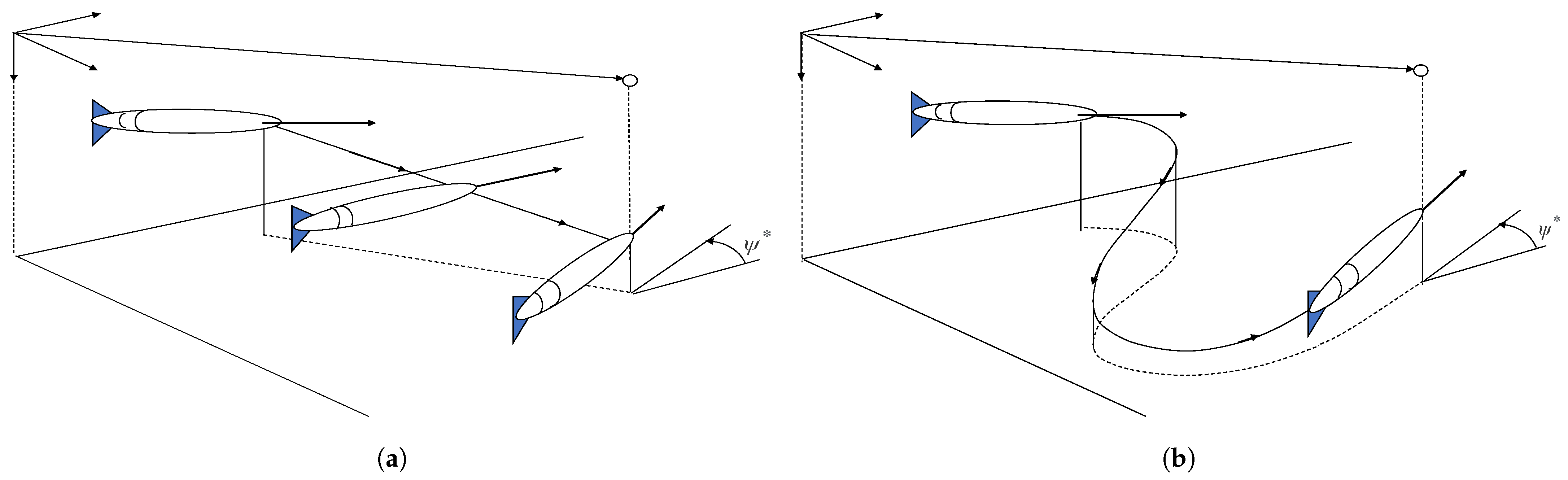
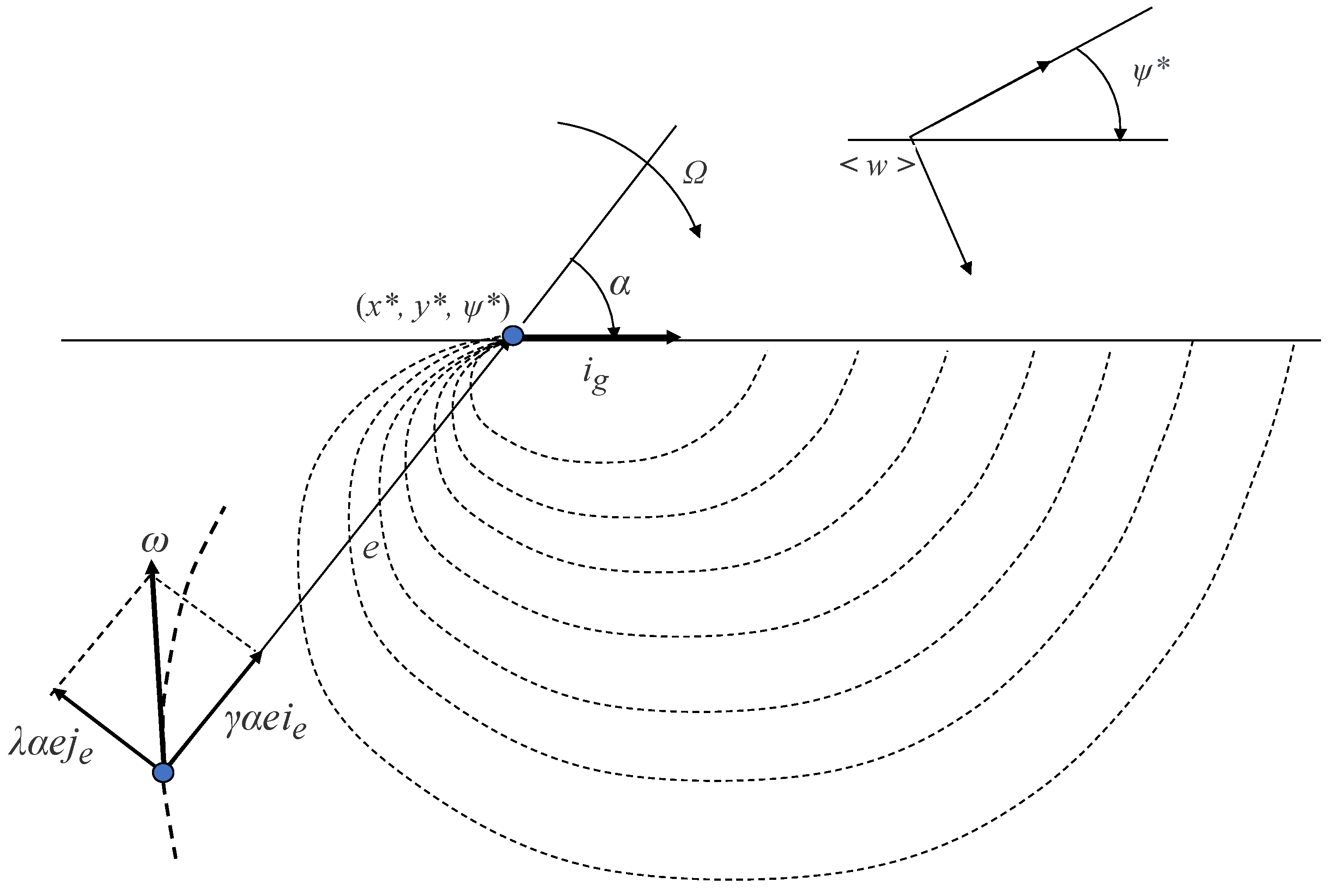
3.2. A Task Priority Approach Integrating Homing and Docking Maneuvers

This section provides an in-depth look on how the various behaviors of our system are achieved in the unified task priority framework. We consider two scenarios as representative of possible missions, one where the AUV executes a constant depth survey (e.g., to simulate the acquisition of acoustic data from the seafloor) and one where the AUV executes a constant altitude survey (e.g., to acquire optical data at a prescribed distance from the seafloor). For this, we introduce various actions such as a parking action ${\mathcal{A}}_p$ to approach the initial way-point for starting the survey mission and also for executing the homing maneuver at the end of the mission; a constant depth survey action ${\mathcal{A}}_{sd}$ and a constant altitude survey ${\mathcal{A}}_{sa}$ action for executing the two survey scenarios; an aligning action ${\mathcal{A}}_a$ that allows the vehicle to orient to the next leg of the survey; and finally a docking action ${\mathcal{A}}_d$ to carry out the docking procedure. The name of the action corresponds to the action defining objective that provides the main functionality. This main functionality, however, does not necessarily need to be the highest priority task in that particular action. On the contrary, it is usually at a low priority, below the tasks which are considered to be related to the safety of the system.

Table 1. List of tasks in actions that encompass the various behaviors of the vehicle. In task type, I refers to an inequality objective and E refers to an equality objective. The numbers denote the priority of each task in their respective action where lower values represent a higher priority for that task in the action.

Task	Task Type	${\mathcal{A}}_{\mathit{p}}$	${\mathcal{A}}_{\mathit{s}\mathit{a}}$	${\mathcal{A}}_{\mathit{s}\mathit{d}}$	${\mathcal{A}}_{\mathit{a}}$	${\mathcal{A}}_{\mathit{d}}$
Minimum Altitude	I	1	1	1
Obstacle Avoidance	I	2	2	2
Horizontal Alignment	I	3
Vehicle Altitude	E		3
Vehicle Depth	E			3
Seafloor Alignment	E	4	4		1
Field Velocity	E	5
Follow 2D Path	E		5	5
Velocity Alignment	E	6	6	6
Hold Position	E				2
Survey Leg Alignment	E				3
Terminal Dock	E					1
Dock Attitude	E					2

provides the list of the tasks and and their priority positioning within the control actions defined and used in this research.

3.3. Description of Tasks within an Action

The following section provides more information on the various tasks composing each one of the above-considered actions, as reported in Table 1. Some tasks are common to multiple actions. For example, the Minimum Altitude Task is common to ${\mathcal{A}}_p$, ${\mathcal{A}}_{sa}$, and ${\mathcal{A}}_{sd}$ actions.

Concerning safety tasks, the Minimum Altitude Task allows the vehicle to maintain a safe altitude above the seafloor. This prevents the vehicle from crashing into the seafloor or other structures below itself. Due to the varying environments through which the vehicle operates, its very likely that it will encounter obstacles along its path. The Obstacle Avoidance Task enables the vehicle to avoid any obstacles along the path. Multiple obstacles are considered, and once they are known with the help of on-board sensors, the task will be able to avoid them in a reactive fashion and proceed towards the goal.

Moving to complementary tasks, the Velocity Alignment Task aligns the longitudinal axis of the vehicle to the reference linear velocity vector. In this way, translations are limited, allowing the main thruster to perform the majority of the work, increasing the overall efficiency as the vehicle moves in the least damping direction. The Alignment to Seafloor Task is a complementary task to the Minimum Altitude Task, and allows the vehicle to follow the terrain and its slope. This helps the vehicle from preventing crashing to the seafloor while maneuvering over rough terrain. This is executed aligning the body z axis to the direction of the seafloor normal ${\mathit{n}}_b$. Details on how the normal can be computed from the specific sensors will be given later in Section 4.1. Furthermore, as it is always convenient not to allow the vehicle to reach high values of pitch, the Horizontal Alignment Task allows the vehicle to control its pitch so that it will not exceed its permissible limits.

Moving to the homing and docking maneuvers, we recall that they can be subdivided into a long-range parking (homing) and a short-range parking (terminal docking) as depicted in Figure 3. The latter can be realized by explicitly taking advantage of the holonomic capabilities exhibited by the vehicle within the execution of short range and slow final maneuvering. For the former maneuver, as already stated, it is instead advisable to reduce translations as much as possible that will otherwise lead to unnecessary energy consumption. This is possible with the help of a velocity field based control. The Field Velocity Task employs the velocity field control discussed in [46,47], recalled in the following. Consider a planar parking problem with a goal at the planar absolute coordinates and absolute yaw angle represented by given and/or measured $x^{*},y^{*},{\psi }^{*}$, as depicted in Figure 4. Then, for constructing a planar horizontal velocity field asymptotically converging towards the goal with the required orientation approach, the angular and linear velocities that are required to drive the position error $\mathit{e}$ (defined in Figure 4) towards zero are of the form

$$\left\{\begin{array}{c}\Omega \doteq \lambda \mathit{\alpha }=\lambda \alpha {\mathit{k}}_{\alpha }\hfill \\ \mathit{w}\doteq \gamma \mathit{e}+(\mathit{e}\wedge \Omega )=\gamma \left|\mathit{e}\right|{\mathit{i}}_e+\lambda \alpha \left|\mathit{e}\right|{\mathit{j}}_e\hfill \\ \doteq {\mathit{w}}_e+{\mathit{w}}_{\Omega }\hfill \end{array}\right.,$$

(15)

where $\alpha$ represents the angle between the position error vector $\mathit{e}$ and goal orientation vector ${\mathit{i}}_g$, and ${\mathit{k}}_{\alpha }$ represents the unit vector along the axis of angle $\mathit{\alpha }$. The linear and angular gains denoted by $\gamma$ and $\lambda$ can be modulated for consequently modulating the rate of convergence of the field by using a parameter $\sigma$ as $\lambda =\sigma \overline{\lambda }$ and $\gamma =\sigma \overline{\gamma }$. Corresponding to the current position of the vehicle, the associated velocity $\mathit{w}$ consequently represents the velocity reference to be tracked by the origin of the vehicle frame $\langle b\rangle$, as well as the heading to be tracked by the same vehicle frame. Thus, the current reference rate $\dot{\overline{\mathit{x}}}$ for the origin of the vehicle body frame simply becomes $\dot{\overline{\mathit{x}}}=\mathit{w}$. Moreover if we need to definitely converge towards a moving docking station, the reference rate will become

$$\dot{\overline{\mathit{x}}}=\mathit{w}+{\mathit{w}}_{\mathit{t}},$$

(16)

where ${\mathit{w}}_{\mathit{t}}$ is the linear velocity of the docking station. For simplicity, we assume that the heading of the docking station remains constant as it is typically the case.

Moreover, as our vehicle is also required to follow this reference velocity by aligning its heading in the velocity direction, let us consider a case when the vehicle is initially misaligned at an angle of $\beta$ with the reference velocity vector. An appropriate angular velocity ${\mathit{\omega }}_{\beta }={\kappa }_{\beta }\beta {\mathit{n}}_{\beta }$ must be applied to reduce the misalignment, where ${\kappa }_{\beta }$ is the gain required to align to the reference velocity vector and ${\mathit{n}}_{\beta }$ is the unit vector normal to the plane containing ${\mathit{\omega }}_{\beta }$. Recalling the Velocity Alignment Task described earlier, it can also be used to achieve such required alignment. Thus, combining the Field Velocity and Velocity Alignment as current references to be tracked, in case of a reliable tracking of both, will allow the vehicle to successfully carry out homing/parking with minimum energy requirements, as the vehicle will eventually move along its minimal drag direction. For extending the 2D planar parking maneuver to a 3D parking maneuver, the 3D parking problem can be reduced to a 2D planar parking problem where the linear field velocity always lie on the plane formed between the linear error vector $\mathit{e}$ and goal orientation vector ${\mathit{i}}_g$ as depicted in Figure 4.

For the very short-range terminal docking, we can exploit the holonomic behavior of the vehicle using a translation maneuver at the final step. As the translation maneuver is used only if absolutely necessary, this can eliminate a lot of drag and energy consumption. The dock location is assumed to be a point (dock position) in free space with an associated orientation (dock orientation) that the vehicle needs to reach with its heading aligned to the dock orientation. To aid the terminal docking maneuver, we define a pre-docking position near the required dock position, at a safe distance from the docking station. A pre-docking position is essentially a point in free space with an associated orientation (pre-docking orientation) that the vehicle needs to reach (in position and orientation) prior to the execution of the docking maneuver. This pre-docking position can be used to attain different dock positions as depicted in Figure 5. Once the vehicle matches its position and orientation to the pre-docking position and orientation with the help of Field Velocity Task and Velocity Alignment Task discussed previously, it gradually surges or translates to the final dock position on the docking station with the help of Terminal Dock Task. To complement the terminal docking maneuver, we use the Dock Attitude Task for maintaining the vehicle orientation to the required dock orientation.

In terms of general mission tasks, we also consider the need for the vehicle to follow a certain path in 2D. For instance, a typical surveying mission might require covering an area by moving in lawn-mowing paths between way-points. The Follow 2D Path Task allows the vehicle to achieve this by implementing the Line of Sight (LOS) [53] path following technique, reducing the along-track and cross-track errors to zero. Such a 2D path following task can be combined with a Vehicle Depth Task, if the survey needs to be conducted at a constant depth, or with a Vehicle Altitude Task, if it needs to be done at constant altitude from the seafloor. Unlike the Minimum altitude task that was discussed before, the Vehicle Depth and the Vehicle Altitude tasks always keep the vehicle altitude or depth close to a reference value. Finally, once the AUV has reached the end of one leg of the survey, we consider a Survey Leg Alignment Task to control the overall attitude of the vehicle, aligning to the next leg while keeping the current position using Hold Position Task before proceeding further with the path following technique. Normally, as these are slow maneuverings, the drag effects remain at very reasonable levels.

4. Simulation Results

This section presents different simulations, which have been carried out to highlight the advantages in using the task-priority framework. In particular, the capability in performing parking and homing maneuvers using the velocity field control technique, the docking maneuver in various challenging scenarios and the mission capability are studied.

4.1. Simulation Setup

The simulation program is written in C++ as it is the programming language that can be used to interface with the real vehicle. The interface to the Simulated System is the same as that of the actual vehicle, allowing for software-in-the-loop simulations of our KCL implementation. Concerning the Planning Layer, we implemented a very basic state machine to handle the sequence of actions.

The vehicle model used in the simulation is the X300 AUV, which is a low-cost torpedo-shaped AUV that is capable of maneuvering with 5 degrees of freedom along the surge, sway, heave, pitch, and yaw directions. The X300 hydrodynamic model is based on the general Fossen model [49,50,51] for an underwater vehicle. The mass and drag parameters of the experimental vehicle X300 have been identified prior to this research. Assuming the vehicle is symmetric in the $x-z$ plane and $y-z$ plane, and almost symmetric in the $x-y$ plane due to relative slow speeds, the origin of vehicle frame coincides with the vehicle center of buoyancy. Various dynamic model parameter terms can thus be simplified as per

Table 2. X300: System Parameters and dynamic model parameters. Thruster distance represents the longitudinal distance of each thruster from the center of body frame.

System Parameter	Value	Model Parameter	Value
DOF	5	Type	Torpedo
Length	2 m	G	9.810
Width	0.15 m	$\rho$	1023.6
Weight	31 kg	CG	[0.000, 0.000, 0.070]
Main Propulsion	Central thruster	CB	[0.000, 0.000, 0.000]
Propellers	5	Added Mass	diag [−0.47, −22.7, −22.7, −0.1, −3.64, −3.64]
		Linear Drag	diag [1.079, 10.21, 10.21, 0.5, 1.061, 1.061]
		Quadratic Drag	diag [0.794, 102.1, 102.1, 20.48, 15.191, 15.191]
		Thruster distance	[−1.0, 0.45, −0.45, 0.6, −0.6]

. The vehicle is powered by 5 thrusters consisting of a main thruster at the aft, 2 lateral thrusters, and 2 vertical thrusters, and thus is not actuated in roll as depicted in Figure 6. The vehicle has its center of mass below its center of buoyancy, allowing the restoring forces to provide passive stability for the vehicle in roll. We also notice that the center of mass is below the line of the thrusters, thereby generating transient roll while translating. However, it should also be noted that we limit translations as much as possible.

The altitude sensors in the vehicle are arranged in the $x-z$ plane of the vehicle as depicted in Figure 7 where they are fixed at 45 degrees forward and aft w.r.t. the vehicle body frame $\langle b\rangle$. These two sensors allows an estimation of the slope of the seafloor by determining the seafloor vector. In the sensor frame $\langle s\rangle$, the rays from the two sensors make contact with seafloor at points ${}^{s}A$ and ${}^{s}B$, respectively. The floor vector $\mathit{f}$ in $\langle b\rangle$ is given as ${}^b\mathit{f}={}^b{\mathit{R}}_s({}^{s}A-{}^{s}B)$, where ${}^b{\mathit{R}}_s$ denotes the rotation matrix from $\langle s\rangle$ to $\langle b\rangle$. The vehicle follows the seafloor terrain by aligning its body z axis in the direction of the orthogonal component ${\mathit{n}}_b$, calculated as a normalized cross-product of the floor vector ${}^b\mathit{f}$ and the body y axis ${\mathit{j}}_b$. It is obvious that the roll could point the altitude sensors far away from the vertical projection of the vehicle on the surface, thereby estimating the slope in another point than the one just below the vehicle. We assume the roll to be negligible because in the design of these kind vehicles, the center of mass and center of buoyancy are located in such a way that the restoring forces provide passive stability in roll. The roll could be further limited by adding fins to make the vehicle more horizontal in terms of roll. For estimating the vehicle altitude, we consider an absolute vertical line, passing through the vehicle body center ${}^{b}O$ and touching the floor vector ${}^b\mathit{f}$ at point ${}^{b}C$. The estimated altitude is the length of the vertical segment $({}^{b}C-{}^{b}O)$.

Table 2 gives a general layout of the vehicle characteristics, including the system and dynamic model parameters.

The dynamics of the vehicle is assumed to be governed by a PI-based velocity control system given by

$$\mathit{u}={\mathit{K}}_p\tilde{\mathit{\nu }}+{\mathit{K}}_i{\int }_{t_0}^t\tilde{\mathit{\nu }}dt,$$

(17)

where $\tilde{\mathit{\nu }}$ is the velocity tracking error (excluding the p angular velocity), and ${\mathit{K}}_p$ and ${\mathit{K}}_i$ are the proportional and integral gain matrices, respectively. The controller is initialized with gains ${\mathit{K}}_p=diag\left([750,780,780,380,100]\right)$ and ${\mathit{K}}_i=diag\left([2280,2310,2310,2000,90]\right)$.

For the simulation, we also assume the availability of sensors (e.g., a forward looking sonar) that are able to compute distances to obstacles when in close proximity with the vehicle for providing feedback to the obstacle avoidance tasks. Moreover, we also assume acoustic communications (e.g., Ultra Short Base Line (USBL) unit with integrated acoustic modem) with the docking station for long range homing and visual markers on the docking station that are recognizable with an on-board camera for terminal docking. We further assume that the vehicle can measure its pose and velocity using on-board sensors (e.g., Inertial Measurement Unit (IMU) and Doppler Velocity Log (DVL)). In case of a moving docking station, its motion is constrained to a straight line motion with a constant heading, and to allow rendezvous, the docking station will be moving with a velocity lower than that of the maximum velocity of the vehicle.

In order to achieve realistic simulations, obstacles are added into the simulation environment. For simplicity, the obstacles are modeled as spheres and the paper is not concerned regarding a fine modeling of the obstacles. As is commonly done, we envelope all the area around the docking place into sphere obstacles for repulsing the vehicle from colliding into structural elements of the station. We can also use these spheres to envelope no-fly zones to represent places or areas where the vehicle should not travel for other reasons than collision risks. For example, to dock to a submarine [31] or an ASV [33], a no fly zone can be defined by placing several spheres around the propeller area of the submarine or ASV so that the vehicle avoids entering into turbulent waters generated by the propulsion system of the submarine or ASV. Clearly when defined w.r.t. the dock location, the spheres will be attached to the dock position body coordinates and would move at the same rate as that of the dock.

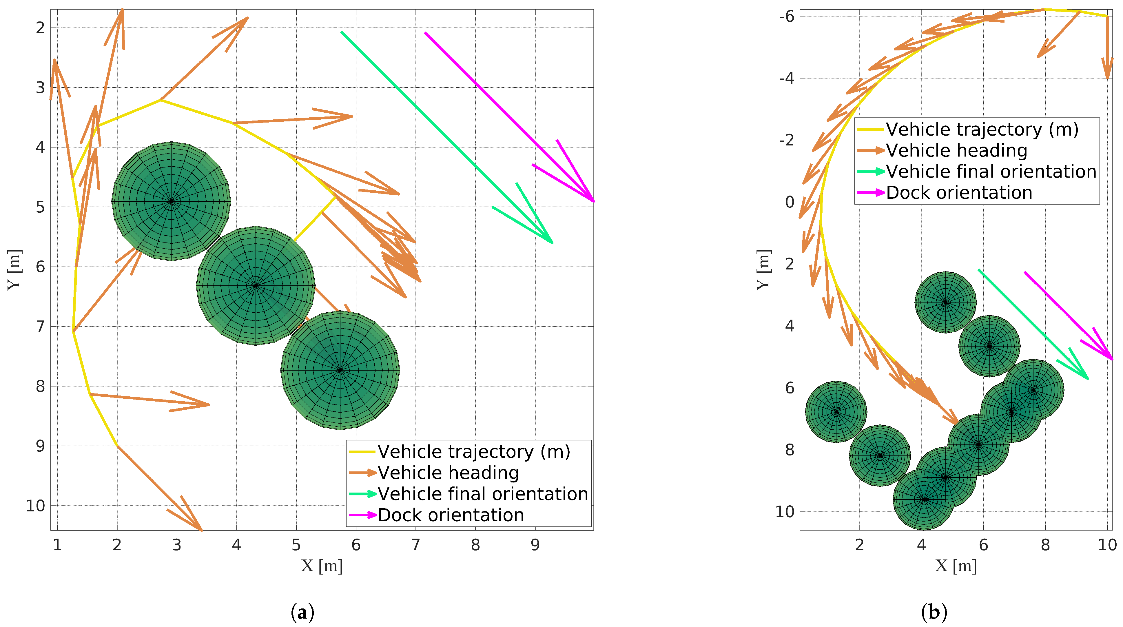
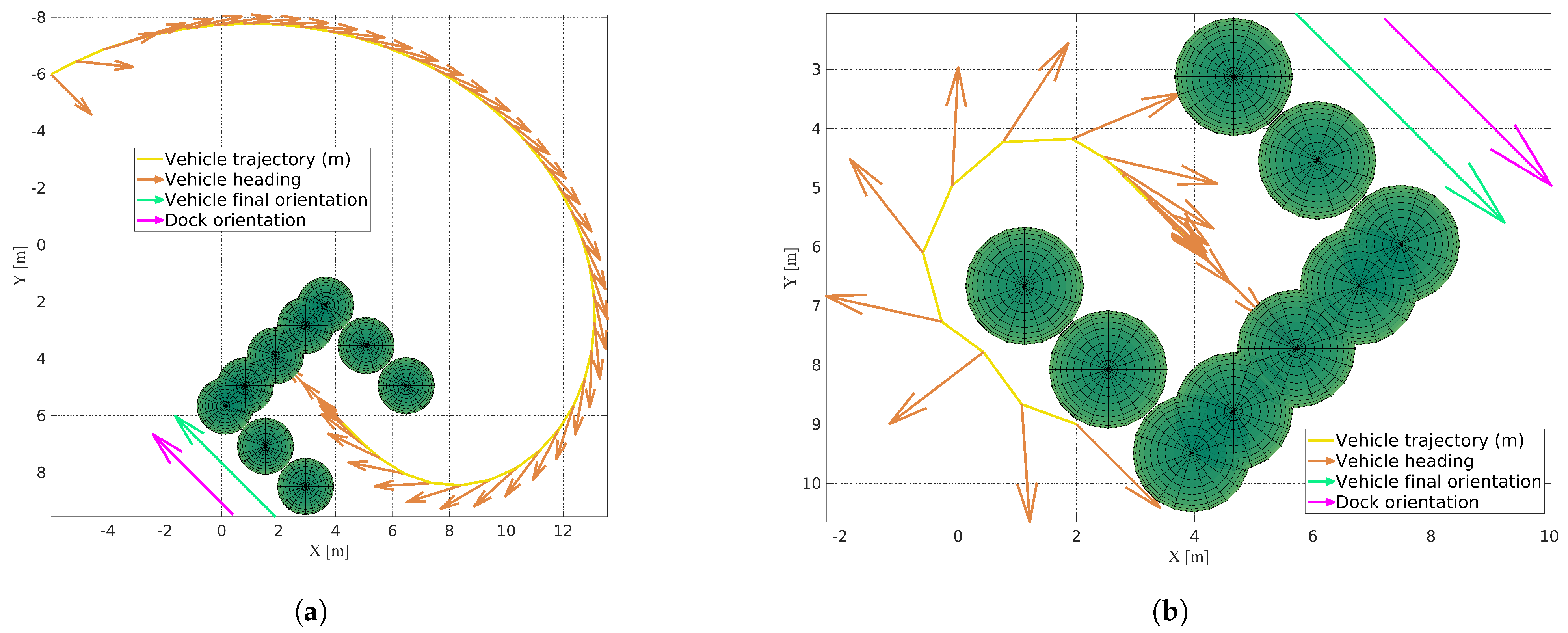
4.2. Free Space Parking and Docking Tests

This section highlights the capability of the system in performing free space parking maneuver (also used for homing) using the velocity field control technique and the capability to perform the docking maneuver in various challenging scenarios. Various trajectories of the vehicle while the parking maneuver is performed in free space with different parameters are presented in Figure 8a. Here, the control parameters—-linear gain $\lambda$, angular gain $\gamma$, and modulation gain $\sigma$—of the task are varied. Increasing the value of $\lambda$ allows the vehicle to reach the goal faster, and increasing the value of $\gamma$ allows the vehicle to achieve the desired orientation sooner. Varying $\sigma$ allows the vehicle to reach the final configuration faster or slower, while following the same path. The result of the free space docking simulations very well portrays how the vehicle perform the parking maneuver for various parameters to obtain the desired target position and orientation irrespective of its initial starting conditions. Action ${\mathcal{A}}_p$ is used for this test.

Figure 8b depicts the behavior of the vehicle while performing a docking maneuver at the bow side of a docking station traveling towards the vehicle. The vehicle follows a curvilinear velocity field trajectory towards the pre-docking position defined at a point in the near-vicinity of the station, and translates to the final dock position for completing the docking maneuver. In comparison to the work in [33], the translation is used only for the terminal docking maneuver, thereby also reducing drag and energy consumption. The ${\mathcal{A}}_p$ and ${\mathcal{A}}_d$ actions are exploited in these tests. The spheres represent the envelope obstacle placed around the docking station to avoid collision as the vehicle moves closer during homing and approach maneuver.

Figure 9a depicts the behavior of the vehicle while performing a docking maneuver around the docking station at close proximity replicating the scenario presented in [30]. Here, the vehicle starts at close proximity from one side of the docking station and travels to the other side of the docking station without colliding with the station. Thanks to the tasks Obstacle avoidance and Field Velocity that are integrated to the task priority framework, the vehicle is able to move away from the close proximity of the station to go around and reach the pre-docking position present on the other side of the station by following a velocity field trajectory before translating to complete the docking maneuver.

Figure 9a and Figure 10a,b show the behavior of the vehicle when it needs to dock into a tight space, such as space-limited docks or piers. The use of pre-docking position allows the vehicle to home into the required orientation for docking without colliding with the surrounding dock structure. In a very extreme situation where the vehicle comes in close proximity with the dock structure, the obstacles and the Obstacle Avoidance task allow the vehicle to safely move away from the dock structure while approaching. Not only do we have the advantage of docking from anywhere and at any initial conditions of the vehicle, but also the ability to avoid any obstacles along the path or avoid crashing into the dock structure.

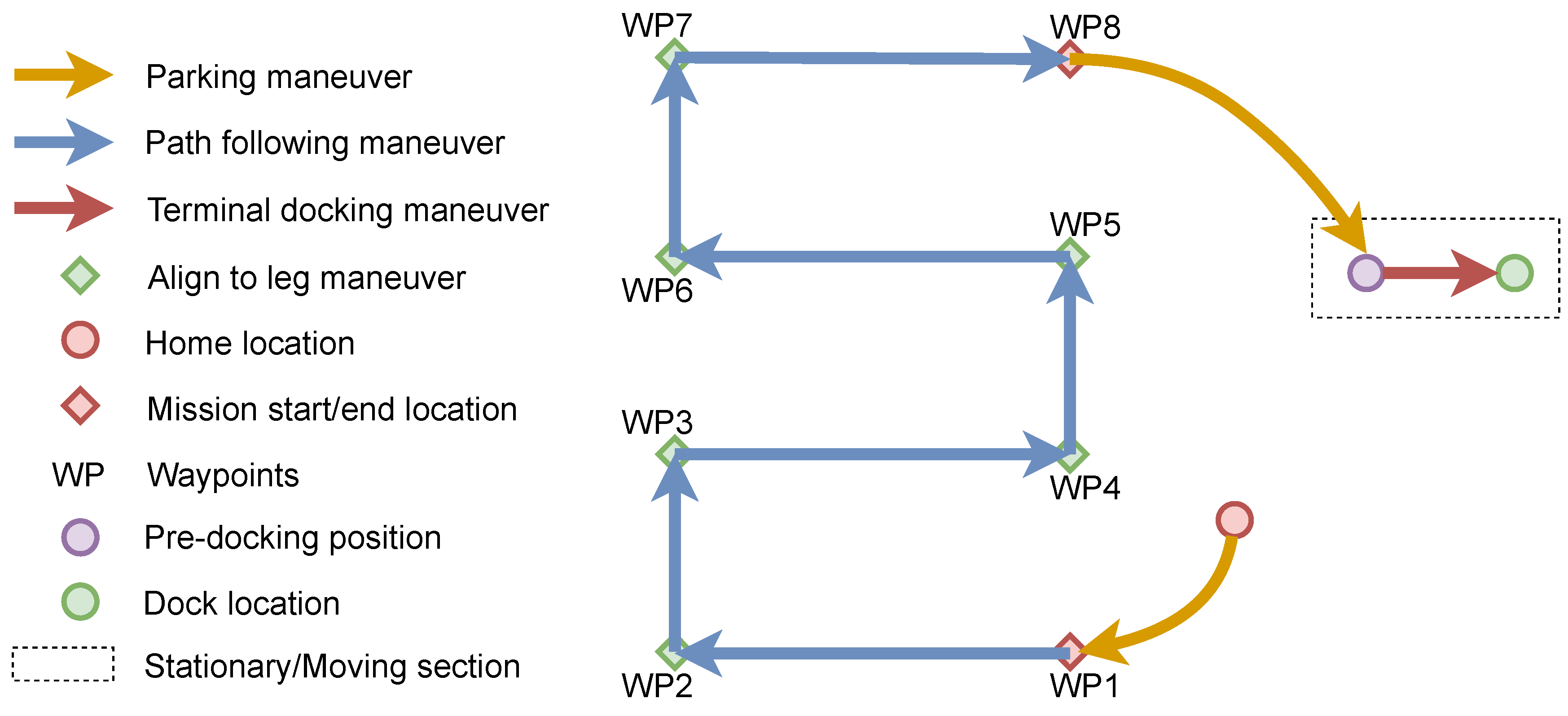
4.3. Vehicle Performing a Complete Mission

This section highlights the simulations encompassing the behaviors of the system in various complex scenarios, using a constant depth survey and constant altitude survey as representative of possible missions, and exploiting the features of task priority framework. These two mission scenarios, which are performed and studied in the following sections, will exploit all the behaviors of the system that were discussed in Section 3. The ability to dock onto a moving docking station is also evaluated in this study. As previously mentioned, a lawn mower profile-based survey is done at constant depth and constant altitude exploiting the LOS path following algorithm [53]. Once the vehicle completes the survey, it homes in to the moving docking station and finally docks. The ${\mathcal{A}}_p$, ${\mathcal{A}}_{sd}$ (for constant depth path following mission), ${\mathcal{A}}_{sa}$ (for constant altitude path following mission), ${\mathcal{A}}_a$, and ${\mathcal{A}}_d$ actions are used for the missions. Some possible ways of docking approaches are depicted in Figure 5. In the missions, we present docking approaches similar to the scenarios taken from [32,33] where the vehicle docks to the moving docking stations from the top and side, respectively. However the classic approach is to dock from the aft of the docking station, e.g., to dock to a towed [31] or funnel-shaped [23] docking station which was already presented in Figure 9b and Figure 10. The dock moves with a constant heading throughout the mission. Ocean current disturbances are also introduced in the following mission simulations.

The missions are carried out as follows. A lawn mower profile is chosen for the survey mission as depicted in Figure 11. Waypoints are inserted wherever the vehicle needs to make a turn during the mission. The waypoint locations, vehicle initial position and orientation, the dock velocity, and the ocean current velocity used in the simulations are reported in

Table 3. Mission parameters. All the positions are defined w.r.t. the world frame.

Parameter	Value
Vehicle initial pose / Home (m, deg)	[−5, −10, 18, 0, 0, 40]
Waypoint 1 pose (m, deg)	[0, −5, 20, 0, 0, 0]
Waypoint 2 pose (m, deg)	[20, −5, 20, 0, 0, 90]
Waypoint 3 pose (m, deg)	[20, 0, 20, 0, 0, 180]
Waypoint 4 pose (m, deg)	[0, 0, 20, 0, 0, 90]
Waypoint 5 pose (m, deg)	[0, 5, 20, 0, 0, 0]
Waypoint 6 pose (m, deg)	[20, 5, 20, 0, 0, 90]
Waypoint 7 pose (m, deg)	[20, 10, 20, 0, 0, 180]
Waypoint 8 pose (m, deg)	[0, 10, 20, 0, 0, 180]
Dock velocity (m/s) (in the dock frame)	[0.3, 0, 0]
Ocean current velocity (m/s) (in the world frame)	[0, 0.2, 0]

. The vehicle starts from the home location and proceeds towards the 1st way-point by following and aligning to the system velocities with the help of action ${\mathcal{A}}_p$. The vehicle transits via each way-point using LOS based control at constant depth using ${\mathcal{A}}_{sd}$ action or constant altitude using ${\mathcal{A}}_{sa}$ action, along with the ${\mathcal{A}}_a$ action. At every stage of the mission, the vehicle reactively avoids the obstacles along its path. A minimum altitude is always maintained to avoid crashing into the seafloor or any bottom structures and while traveling close to seafloor, the vehicle follows the terrain to avoid crashing into it when maneuvering over rough terrain. Once the vehicle completes its mission, the homing stage will start using the action ${\mathcal{A}}_p$. The action will drive the AUV to the associated pre-docking position, defined w.r.t. the docking station as stated earlier. Thanks to the tasks defined in action ${\mathcal{A}}_p$, the vehicle will align its heading to the system velocities as it proceeds towards the pre-docking position, while gradually aligning to the terminal orientation too. Once the misalignment errors are within the acceptable range, the vehicle surges or translates towards the final dock position with the help of action ${\mathcal{A}}_d$.

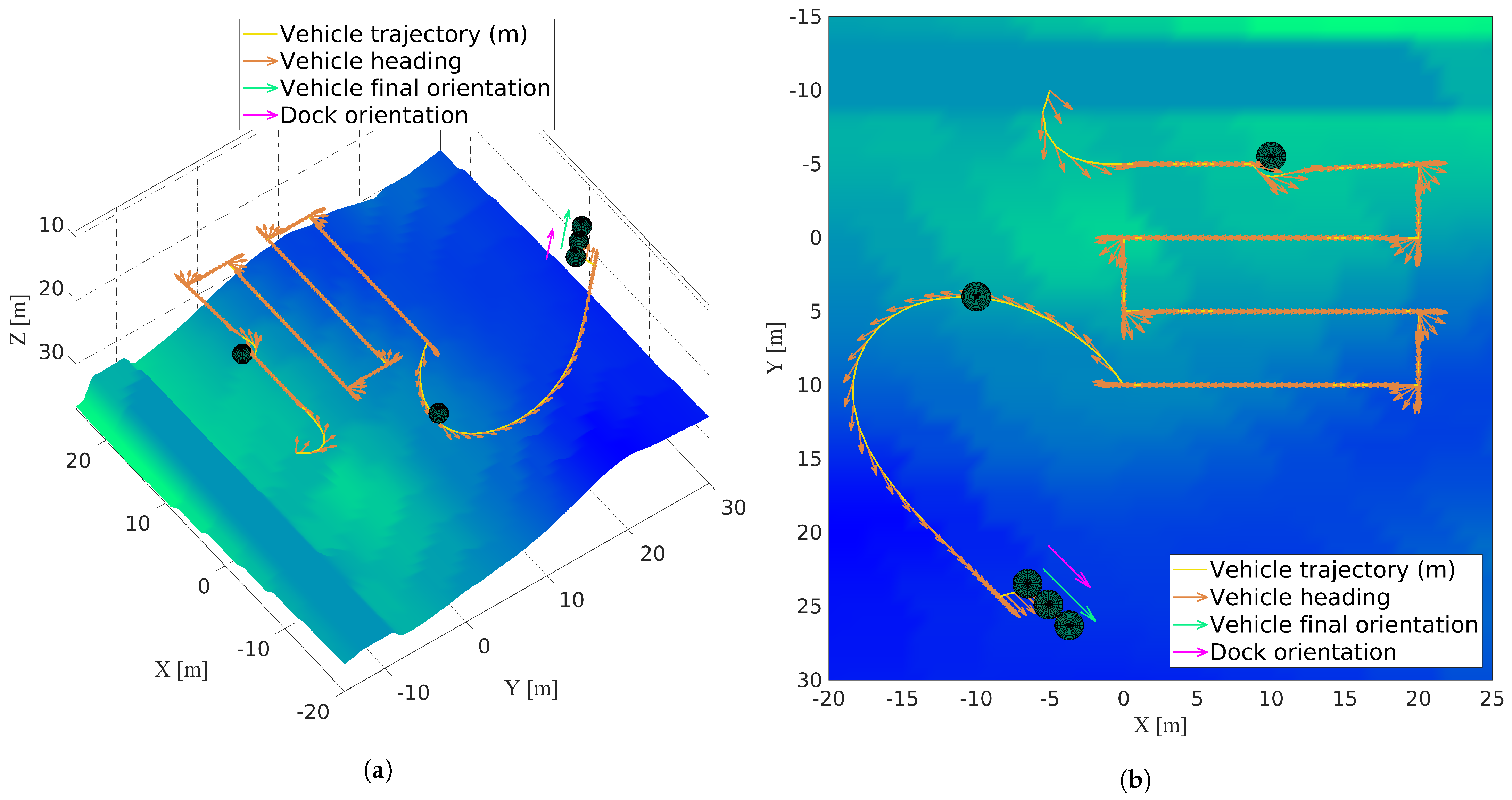
4.3.1. Constant Depth Mission with Docking to a Moving Docking Station Close to the Surface

Here, the vehicle performs a survey mission at constant depth. Figure 12a,b shows the vehicle performing the mission, homing and then docking to a moving docking station close to the surface. The vehicle performs the constant depth survey mission (${\mathcal{A}}_{sd}$ and ${\mathcal{A}}_a$) by maintaining a predefined depth throughout the mission. The Seafloor Alignment Task in the ${\mathcal{A}}_a$ action is disabled while performing the constant depth survey mission phase. Once the mission is completed, the vehicle enters homing phase (${\mathcal{A}}_p$) and returns to the docking station situated close to the seafloor. The vehicle is required to dock to the starboard side of the moving docking station and hence the pre-docking position is placed at a position to the right of the required dock position on the docking station. Here, as the vehicle starts the homing phase, the docking station is moving in front of the vehicle in the opposite direction. As the orientation error in yaw is high and thanks to the Field Velocity Task, the vehicle will make a wider turn while approaching the starboard side of the moving dock as seen in Figure 12. The vehicle, after matching its position and orientation with the pre-docking position and orientation using velocity field, eventually translates sideways to the final dock position on the vehicle (${\mathcal{A}}_d$). At every phase, the vehicle reactively avoids the obstacles along its path. The spheres depicted around the docking station is the envelope obstacle to provide a safety area around the docking station while the vehicle approaches the dock during homing. It is also used for guiding the vehicle towards the required approach position for a safe docking.

From Figure 13, at around time $t=20$, the vehicle changes from the parking maneuver (${\mathcal{A}}_p$) to the path following at constant depth survey maneuver (${\mathcal{A}}_{sd}$ and ${\mathcal{A}}_a$). At time $t=336$, the vehicle starts the homing maneuver (${\mathcal{A}}_p$), and at time $t=374$, the docking maneuver (${\mathcal{A}}_d$) is initiated. During the mission, the depth of the vehicle is maintained at the desired level by the Vehicle Depth task. However, the vehicle encounters two obstacles along its path as depicted by spheres at positions [10, −5.5, 20.5] and [−10, 4, 17]. Obstacle avoidance data from Figure 13 shows that the vehicle is able to estimate the distance to the obstacles (only the distance to the nearest obstacle at each instant is plotted) and reactively avoids them along the path. Looking at Figure 12, notice how the obstacle found during the homing stage is avoided by traveling beneath it, due to the availability of free space without conflicting with the desired minimum altitude from the seafloor. Figure 14 highlights the time behavior of the tasks that are used in the mission (Obstacle Avoidance, Minimum Altitude, and Vehicle Depth) and homing (Obstacle Avoidance, Minimum Altitude, and Seafloor Alignment) phases. In this mission, the roll values of the vehicle vary from −4 degrees to 4 degrees, therefore confirming that the roll angles are negligible and acceptable. Figure 15 depict the time behavior of desired velocities and the actual/system velocities of the vehicle. From the plots, it can be noticed how the translation on the lateral and vertical axis are mainly of a transient nature, with the exception of the terminal docking phase.

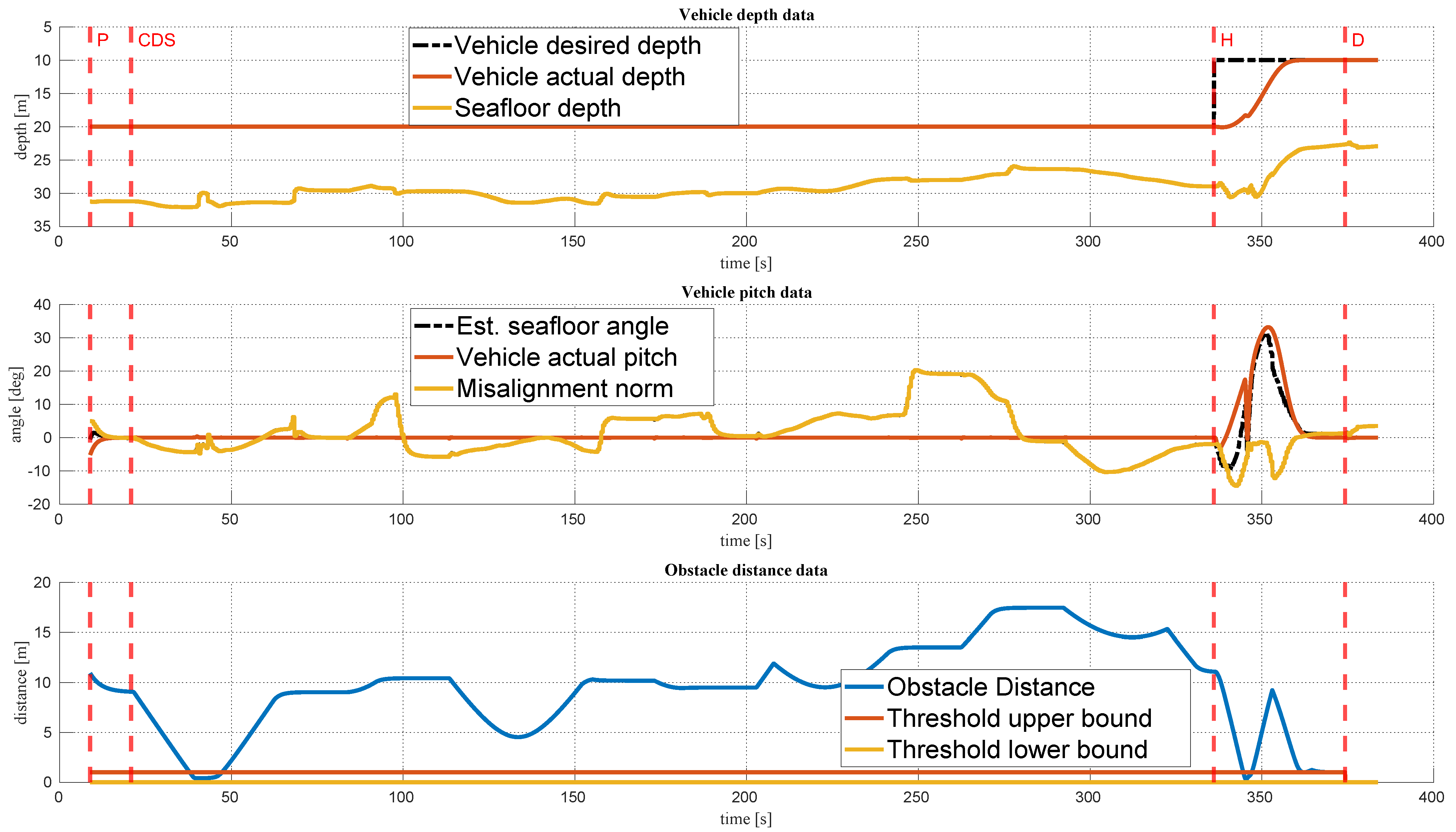
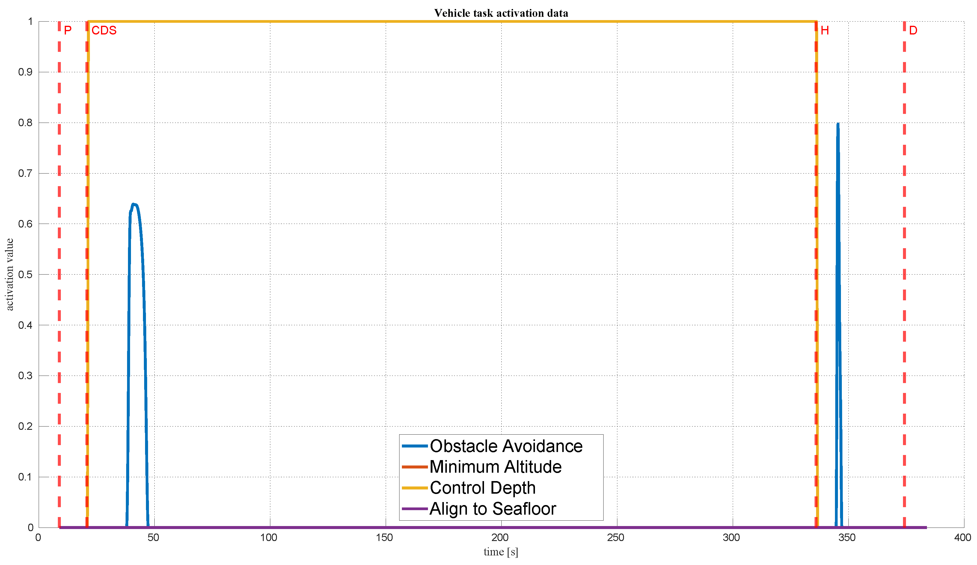
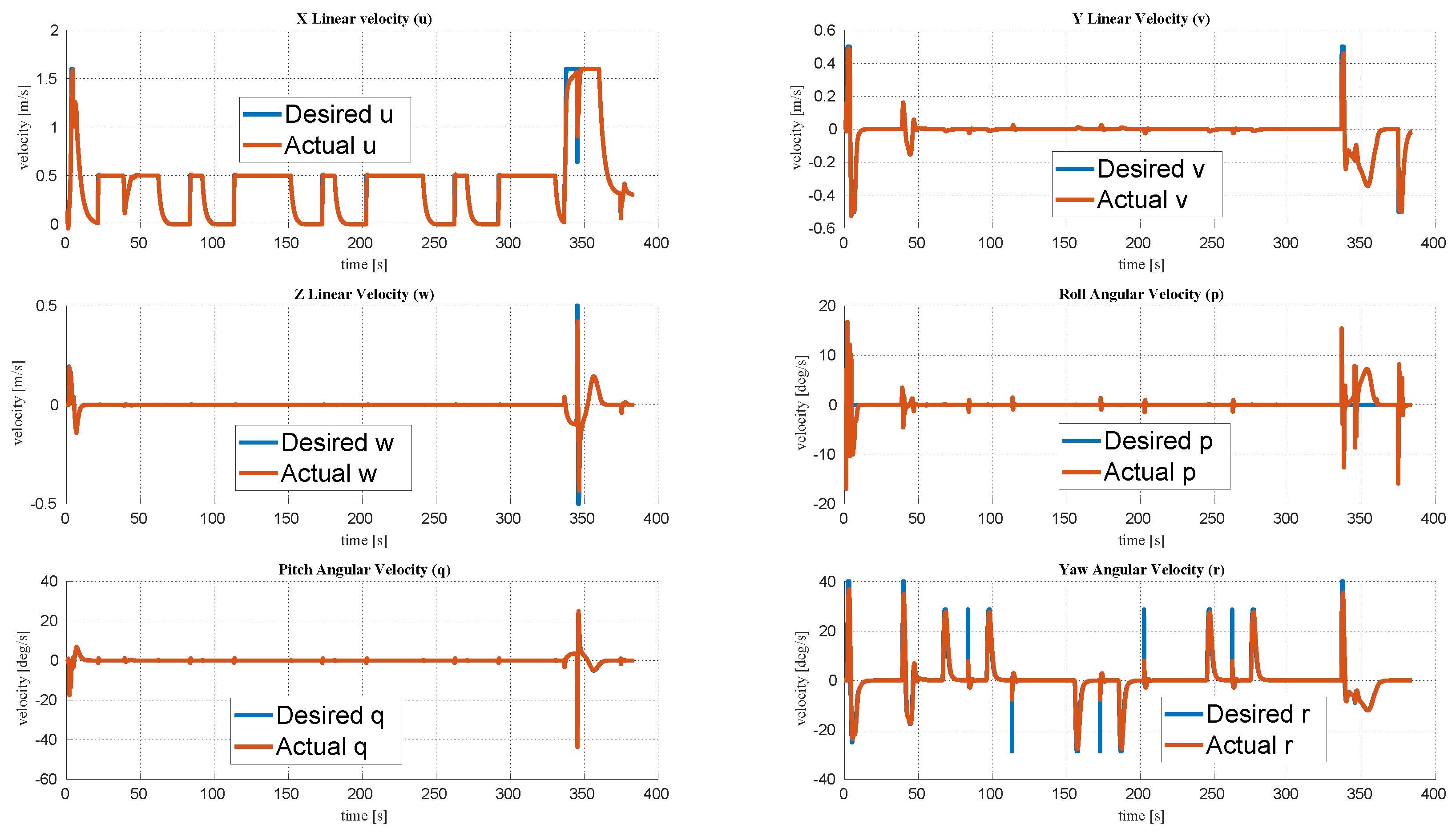
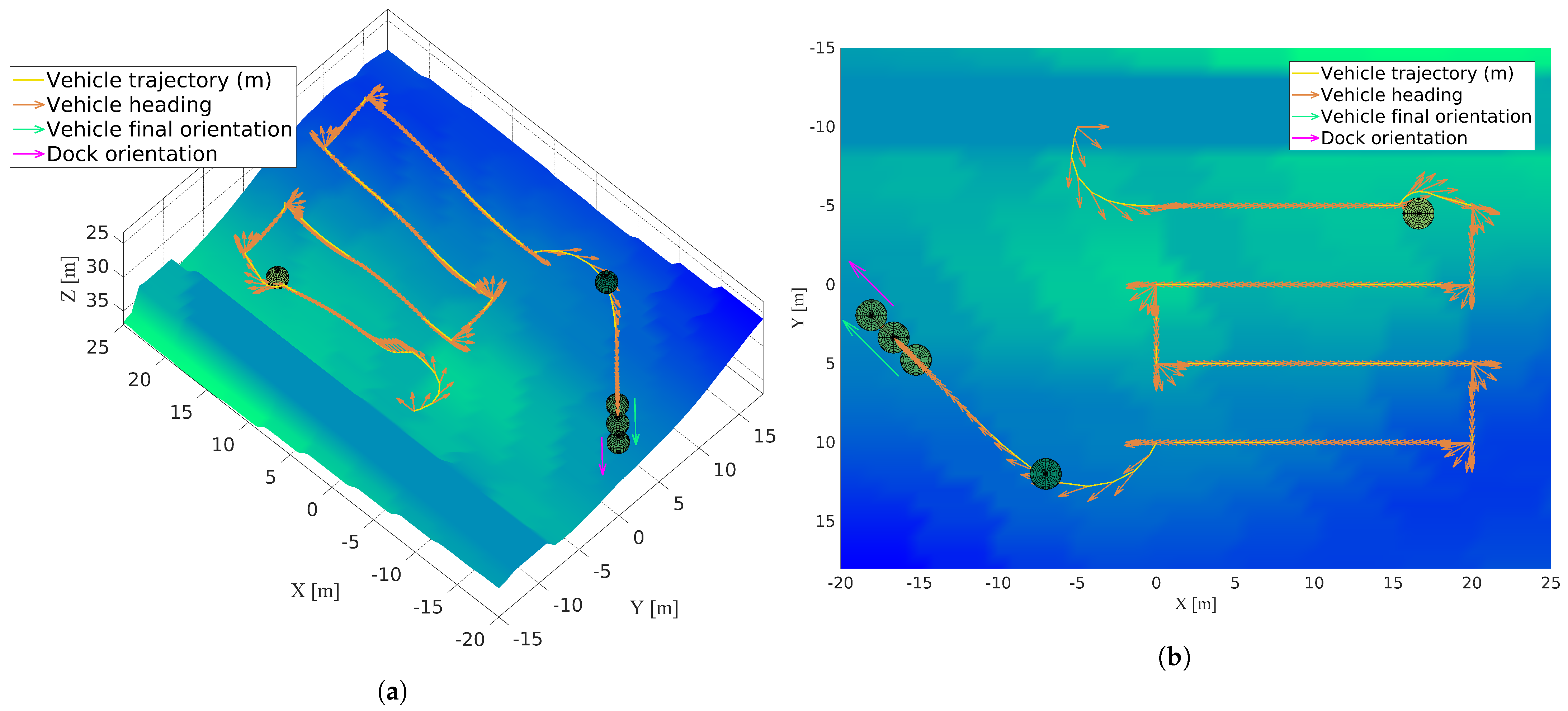
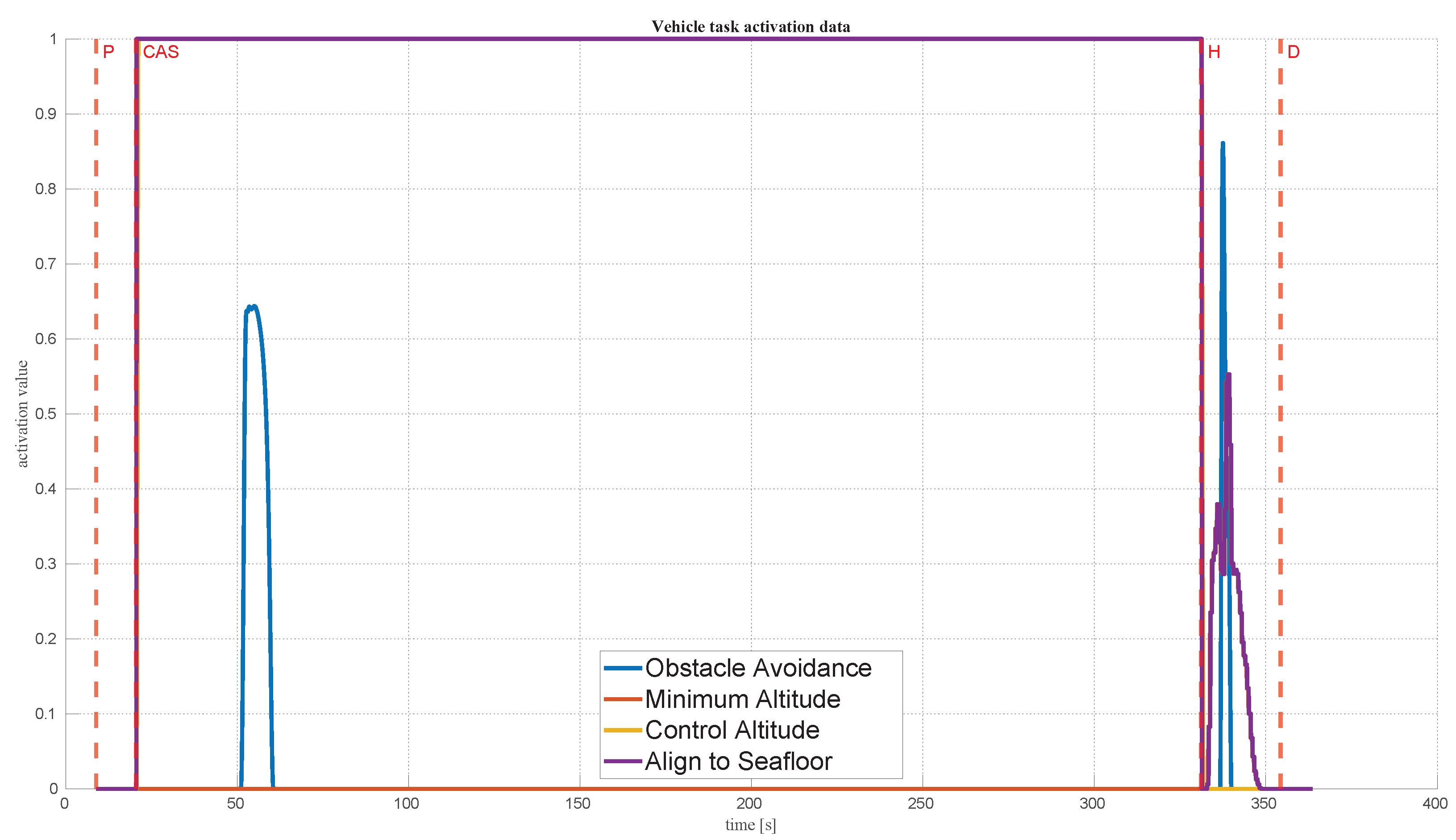
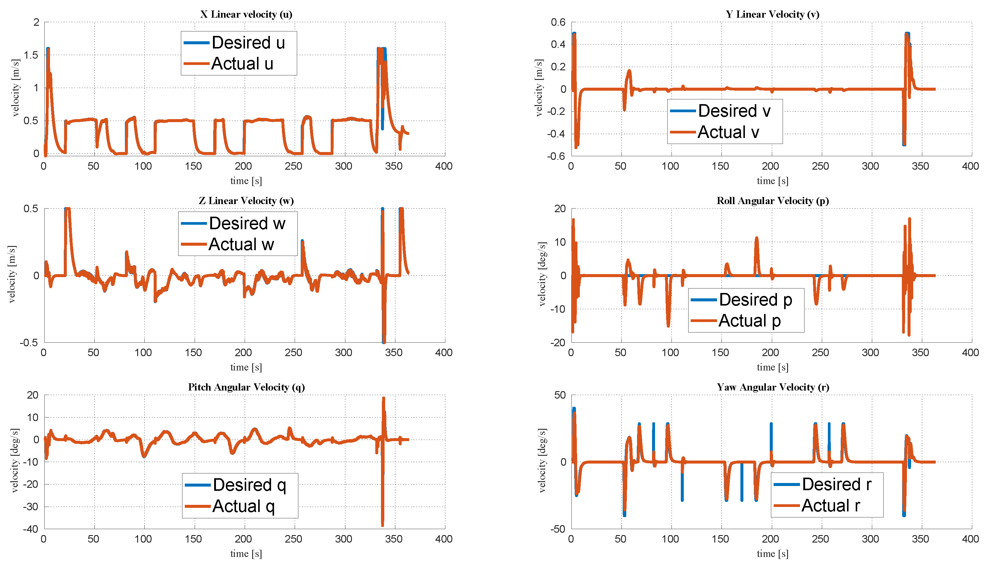
4.3.2. Constant Altitude Mission with Terrain Following and Docking to a Moving Docking Station Situated Close to the Seafloor

For inspection surveys, the vehicle needs to travel at a certain altitude above to the seafloor for gathering data with distance-dependent sensors such as vision sensors. A constant altitude survey is performed in such scenarios. Figure 16a,b shows the complete behavior of the vehicle performing a constant altitude survey mission (${\mathcal{A}}_{sa}$ and ${\mathcal{A}}_a$), homing (${\mathcal{A}}_p$), and finally docking (${\mathcal{A}}_d$) to a docking station moving at a depth close to the seafloor. The vehicle maintains a predefined altitude from the seafloor throughout the mission, it follows the terrain of the seafloor (an improvement over [32]) and also avoids various obstacles along its path. Once the vehicle completes the mission, it enters homing phase. Here, the AUV is required to dock on top of the docking station, therefore the pre-docking position is placed above the required dock position at a safety distance. The vehicle matches its position and orientation with the pre-docking position and orientation with the help of velocity field and eventually translates down to the final dock position on top the docking station. The spheres depicted around the docking station is the envelope obstacle to provide a safety area around the docking station for avoiding any collision with the docking structure as the vehicle approaches the dock while homing. In this survey mission, upon reaching a way-point, the vehicle can maintain its pitch aligned to the terrain of the seafloor even while orienting towards the next leg of the survey (${\mathcal{A}}_a$). However, one can easily change this behavior and require the AUV to maintain a horizontal attitude, while it orients towards the next leg of the survey, by simply deactivating the Seafloor Alignment Task in ${\mathcal{A}}_a$ action. This is possible only because of the flexibility of the task priority approach in introducing specific behaviors to the vehicle.

From Figure 17, at around time $t=20$, the vehicle transitions from the parking maneuver (${\mathcal{A}}_p$) to the path following using constant altitude survey maneuver (${\mathcal{A}}_{sa}$ and ${\mathcal{A}}_a$). At time $t=331$, the vehicle enters homing maneuver (${\mathcal{A}}_p$) and at time $t=354$, the docking maneuver (${\mathcal{A}}_d$) is initiated. The vehicle depth is represented as the altitude of vehicle above the seafloor and it is clear that the vehicle maintains a specific altitude above the seafloor with the help of Vehicle Altitude task during all phases of the mission. Maintaining a safe minimum altitude from the seafloor is further carried out by the Minimum Altitude Task during the homing phase. The vehicle pitch data show the variation of pitch orientation of the vehicle while it follows the terrain of the seafloor. However, due to the pitch limitation implemented via Horizontal Alignment Task, the vehicle pitch does not increase beyond its permissible limits. The vehicle encounters two obstacles along its path as depicted by spheres at positions [16.6, −4.5, 32.5] and [−7, 12, 27]. Obstacle avoidance data from Figure 17 show that the vehicle is able to estimate the distance to the obstacles (only the distance to the nearest obstacle at each instant is plotted) and reactively avoids them along the path. Looking at Figure 16, notice again that the obstacle found during the homing stage is avoided by traveling beneath it, due to the availability of free space without conflicting with the desired minimum altitude from the seafloor. Figure 18 highlights the time behavior of the tasks that are used in the mission (Obstacle Avoidance, Minimum Altitude, Vehicle Altitude, Seafloor Alignment), and homing (Obstacle Avoidance, Minimum Altitude, and Seafloor Alignment) phases. In this mission, the roll values of the vehicle is found to vary from −4.5 degrees to 6 degrees, therefore confirming that the roll angles are negligible and acceptable. Figure 19 depict the time behavior of desired velocities and the actual/system velocities of the vehicle.

5. Conclusions

In this research, we focused on the problems arising when AUVs are required to execute a mission and autonomously home and dock to stationary or moving docking stations, and have shown how to tackle them using a common framework approach. We presented a general control strategy incorporating various vehicle behaviors into the task priority framework, targeting a system capable of staying and operating underwater, perform autonomous missions, homing, docking, obstacle avoidance, terrain following, minimum altitude, and pitch control. The paper has presented the tasks and actions with proper priorities defined to achieve the various vehicle behaviors. In particular, we have shown how to integrate the Field Velocity Task for long-range parking maneuver, allowing the AUV to reach the close proximity of the docking station oriented well in advance. Furthermore, we have shown how the adoption of the task-priority framework allows to integrate tasks such as Obstacle Avoidance or Seafloor Alignment and exploit them both during the execution of the regular survey mission, but also while doing the homing and docking maneuvers; therefore, tackling these maneuvers in more challenging conditions w.r.t. previous works. The contributions have been shown thanks to different numerical simulations, based on the hydrodynamic model of the X300 AUV, demonstrating the successful integrated execution of surveying, homing and terminal docking maneuvers. The results very well prove that the proposed framework is flexible as additional capabilities to the system can be incorporated very easily. This architecture is ready to be expanded to manipulation tasks in the future [37,41].

References

1. Wynn, R.B.; Huvenne, V.A.I.; Le Bas, T.P.; Murton, B.J.; Connelly, D.P.; Bett, B.J.; Ruhl, H.A.; Morris, K.J.; Peakall, J.; Parsons, D.R.; et al. Autonomous Underwater Vehicles (AUVs): Their past, present and future contributions to the advancement of marine geoscience. Mar. Geol. 2014, 352, 451–468. [Google Scholar] [CrossRef] [Green Version]
2. Nicholson, J.W.; Healey, A.J. The Present State of Autonomous Underwater Vehicle (AUV) Applications and Technologies. Mar. Technol. Soc. J. 2008, 42, 44–51. [Google Scholar] [CrossRef]
3. Joye, S.B. Deepwater Horizon, 5 years on. Science 2015, 349, 592–593. [Google Scholar] [CrossRef]
4. Anderson, B.; Crowell, J. Workhorse AUV—A cost-sensible new Autonomous Underwater Vehicle for Surveys/Soundings, Search & Rescue, and Research. In Proceedings of the OCEANS 2005 MTS/IEEE, Washington, DC, USA, 17–23 September 2005. [Google Scholar] [CrossRef]
5. Marani, G.; Choi, S.K.; Yuh, J. Underwater autonomous manipulation for intervention missions AUVs. Ocean Eng. 2009, 36, 15–23. [Google Scholar] [CrossRef]
6. Palomeras, N.; Vallicrosa, G.; Mallios, A.; Bosch, J.; Vidal, E.; Hurtos, N.; Carreras, M.; Ridao, P. AUV homing and docking for remote operations. Ocean Eng. 2018, 154, 106–120. [Google Scholar] [CrossRef]
7. Song, Z.; Marburg, A.; Manalang, D. Resident Subsea Robotic Systems: A Review. Mar. Technol. Soc. J. 2020, 54. [Google Scholar] [CrossRef]
8. Martin, A.Y. Unmanned Maritime Vehicles: Technology Evolution and Implications. Mar. Technol. Soc. J. 2013, 47. [Google Scholar] [CrossRef]
9. Newell, T. Technical Building Blocks for a Resident Subsea Vehicle. In Proceedings of the Offshore Technology Conference, Houston, TX, USA, 30 April–3 May 2018. [Google Scholar] [CrossRef]
10. Curtin, T.; Manalang, D. Resident Autonomous Underwater Vehicles: Docking Revisited. In Proceedings of the 2018 IEEE/OES Autonomous Underwater Vehicle Workshop (AUV), Porto, Portugal, 6–9 November 2018; pp. 1–6. [Google Scholar] [CrossRef]
11. Manalang, D.; Delaney, J.; Marburg, A.; Nawaz, A. Resident AUV Workshop 2018: Applications and a Path Forward. In Proceedings of the 2018 IEEE/OES Autonomous Underwater Vehicle Workshop (AUV), Porto, Portugal, 6–9 November 2018; pp. 1–6. [Google Scholar] [CrossRef]
12. Jacobs, T. Robotic Roustabouts for Tomorrow’s Subsea Fields. J. Pet. Technol. 2014, 66, 50–55. [Google Scholar] [CrossRef]
13. Gilmour, B.; Niccum, G.; O’Donnell, T. Field resident AUV systems—Chevron’s long-term goal for AUV development. In Proceedings of the 2012 IEEE/OES Autonomous Underwater Vehicles (AUV), Southampton, UK, 24–27 September 2012. [Google Scholar] [CrossRef]
14. Zagatti, R.; Juliano, D.R.; Doak, R.; Souza, G.M.; de Paula Nardy, L.; Lepikson, H.A.; Gaudig, C.; Kirchner, F. FlatFish Resident AUV: Leading the Autonomy Era for Subsea Oil and Gas Operations. In Proceedings of the Offshore Technology Conference, Houston, TX, USA, 30 April–3 May 2018. [Google Scholar] [CrossRef]
15. Matsuda, T.; Maki, T.; Masuda, K.; Sakamaki, T. Resident autonomous underwater vehicle: Underwater system for prolonged and continuous monitoring based at a seafloor station. Robot. Auton. Syst. 2019, 120, 103231. [Google Scholar] [CrossRef]
16. Furuholmen, M.; Hanssen, A.; Carter, R.; Hatlen, K.; Siesjo, J. Resident Autonomous Underwater Vehicle Systems—A Review of Drivers, Applications, and Integration Options for the Subsea Oil and Gas Market. In Proceedings of the Offshore Mediterranean Conference, Ravenna, Italy, 20–22 March 2013. [Google Scholar]
17. Sarda, E.I.; Dhanak, M.R. A USV-Based Automated Launch and Recovery System for AUVs. IEEE J. Ocean. Eng. 2016, 42, 37–55. [Google Scholar] [CrossRef]
18. Ahmad, S.M.; Sutton, R.; Burns, R. Retrieval of an Autonomous Underwater Vehicle: An Interception Approach. Underw. Technol. Int. J. Soc. Underw. 2003, 25, 185–197. [Google Scholar] [CrossRef]
19. Hardy, T.; Barlow, G. Unmanned Underwater Vehicle (UUV) deployment and retrieval considerations for submarines. In Proceedings of the International Naval Engineering Conference and Exhibition, Hamburg, Germany, 1–3 April 2008. [Google Scholar]
20. Renilson, M. A simplified concept for recovering a UUV to a submarine. Underw. Technol. Int. J. Soc. Underw. 2014, 32, 193–197. [Google Scholar] [CrossRef] [Green Version]
21. Stuart, H.; Wang, S.; Khatib, O.; Cutkosky, M.R. The Ocean One hands: An adaptive design for robust marine manipulation. Int. J. Robot. Res. 2017, 36, 150–166. [Google Scholar] [CrossRef]
22. Simetti, E. Autonomous Underwater Intervention. Curr. Robot. Rep. 2020, 1, 117–122. [Google Scholar] [CrossRef]
23. Stokey, R.; Purcell, M.; Forrester, N.; Austin, T.; Goldsborough, R.; Allen, B.; von Alt, C. A docking system for REMUS, an autonomous underwater vehicle. In Proceedings of the OCEANS’97. MTS/IEEE Conference Proceedings, Halifax, NS, Canada, 6–9 October 1997; Volume 2, pp. 1132–1136. [Google Scholar]
24. Vu, M.T.; Choi, H.S.; Nhat, T.Q.M.; Nguyen, N.D.; Lee, S.D.; Le, T.H.; Sur, J. Docking assessment algorithm for autonomous underwater vehicles. Appl. Ocean Res. 2020, 100, 102180. [Google Scholar] [CrossRef]
25. Maire, F.D.; Prasser, D.; Dunbabin, M.; Dawson, M. A vision based target detection system for docking of an autonomous underwater vehicle. In Proceedings of the 2009 Australasion Conference on Robotics and Automation, Sydney, Australia, 2–4 December 2009. [Google Scholar]
26. Cowen, S.; Briest, S.; Dombrowski, J. Underwater docking of autonomous undersea vehicles using optical terminal guidance. In Proceedings of the OCEANS’97, MTS/IEEE Conference Proceedings, Halifax, NS, Canada, 6–9 October 1997; Volume 2, pp. 1143–1147. [Google Scholar]
27. Trslić, P.; Weir, A.; Riordan, J.; Omerdic, E.; Toal, D.; Dooly, G. Vision-Based Localization System Suited to Resident Underwater Vehicles. Sensors 2020, 20, 529. [Google Scholar] [CrossRef] [PubMed] [Green Version]
28. Brignone, L.; Perrier, M.; Viala, C. A fully autonomous docking strategy for intervention AUVs. In Proceedings of the OCEANS 2007-Europe, Aberdeen, Scotland, 18–21 June 2007; pp. 1–6. [Google Scholar]
29. Vandavasi, B.N.J.; Arunachalam, U.; Narayanaswamy, V.; Raju, R.; Vittal, D.P.; Muthiah, R.; Gidugu, A.R. Concept and testing of an electromagnetic homing guidance system for autonomous underwater vehicles. Appl. Ocean Res. 2018, 73, 149–159. [Google Scholar] [CrossRef]
30. Woo, J.; Kim, N. Vector Field based Guidance Method for Docking of an Unmanned Surface Vehicle. In Proceedings of the Twelfth ISOPE Pacific/Asia Offshore Mechanics Symposium, Gold Coast, Australia, 4–7 October 2016. [Google Scholar]
31. Sujit, P.B.; Healey, A.J.; Sousa, J.B. AUV docking on a moving submarine using a K-R navigation function. In Proceedings of the 2011 IEEE/RSJ International Conference on Intelligent Robots and Systems, San Francisco, CA, USA, 25–30 September 2011. [Google Scholar] [CrossRef]
32. Yan, Z.; Xu, D.; Chen, T.; Zhou, J.; Wei, S.; Wang, Y. Modeling, strategy and control of UUV for autonomous underwater docking recovery to moving platform. In Proceedings of the 2017 36th Chinese Control Conference (CCC), Dalian, China, 26–28 July 2017. [Google Scholar] [CrossRef]
33. Breivik, M.; Loberg, J.E. A Virtual Target-Based Underway Docking Procedure for Unmanned Surface Vehicles. IFAC Proc. Vol. 2011, 44, 13630–13635. [Google Scholar] [CrossRef] [Green Version]
34. Siciliano, B.; Slotine, J.J.E. A general framework for managing multiple tasks in highly redundant robotic systems. In Proceedings of the Fifth International Conference on Advanced Robotics ’Robots in Unstructured Environments, Pisa, Italy, 19–22 July 1991. [Google Scholar] [CrossRef]
35. Lee, J.; Mansard, N.; Park, J. Intermediate Desired Value Approach for Task Transition of Robots in Kinematic Control. IEEE Trans. Robot. 2012, 28, 1260–1277. [Google Scholar] [CrossRef]
36. Moe, S.; Antonelli, G.; Teel, A.R.; Pettersen, K.Y.; Schrimpf, J. Set-Based Tasks within the Singularity-Robust Multiple Task-Priority Inverse Kinematics Framework: General Formulation, Stability Analysis, and Experimental Results. Front. Robot. AI 2016, 3. [Google Scholar] [CrossRef]
37. Simetti, E.; Casalino, G.; Wanderlingh, F.; Aicardi, M. Task priority control of underwater intervention systems: Theory and applications. Ocean Eng. 2018, 164, 40–54. [Google Scholar] [CrossRef]
38. Cieślak, P.; Simoni, R.; Ridao Rodríguez, P.; Youakim, D. Practical formulation of obstacle avoidance in the Task-Priority framework for use in robotic inspection and intervention scenarios. Robot. Auton. Syst. 2020, 124, 103396. [Google Scholar] [CrossRef]
39. Simetti, E.; Casalino, G. A Novel Practical Technique to Integrate Inequality Control Objectives and Task Transitions in Priority Based Control. J. Intell. Robot. Syst. 2016, 84, 877–902. [Google Scholar] [CrossRef]
40. Simetti, E.; Wanderlingh, F.; Torelli, S.; Bibuli, M.; Odetti, A.; Bruzzone, G.; Rizzini, D.L.; Aleotti, J.; Palli, G.; Moriello, L.; et al. Autonomous Underwater Intervention: Experimental Results of the MARIS Project. IEEE J. Ocean. Eng. 2018, 43, 620–639. [Google Scholar] [CrossRef]
41. Di Lillo, P.; Simetti, E.; Wanderlingh, F.; Casalino, G.; Antonelli, G. Underwater Intervention With Remote Supervision via Satellite Communication: Developed Control Architecture and Experimental Results Within the Dexrov Project. IEEE Trans. Control Syst. Technol. 2020, 29, 102–123. [Google Scholar] [CrossRef]
42. Di Vito, D.; De Palma, D.; Simetti, E.; Indiveri, G.; Antonelli, G. Experimental validation of the modeling and control of a multibody underwater vehicle manipulator system for sea mining exploration. J. Field Robot. 2020. [Google Scholar] [CrossRef]
43. Simetti, E.; Campos, R.; Di Vito, D.; Quintana, J.; Antonelli, G.; Garcia, R.; Turetta, A. Sea Mining Exploration with an UVMS: Experimental Validation of the Control and Perception Framework. IEEE/ASME Trans. Mechatronics 2020, 1. [Google Scholar] [CrossRef]
44. Simetti, E.; Casalino, G. Manipulation and Transportation With Cooperative Underwater Vehicle Manipulator Systems. IEEE J. Ocean. Eng. 2016, 42, 782–799. [Google Scholar] [CrossRef]
45. Simetti, E.; Casalino, G.; Wanderlingh, F.; Aicardi, M. A task priority approach to cooperative mobile manipulation: Theory and experiments. Robot. Auton. Syst. 2019, 122, 103287. [Google Scholar] [CrossRef]
46. Aicardi, M.; Cannata, G.; Casalino, G.; Indiveri, G. Guidance of 3d underwater nonholonomic vehicle via projection on holonomic solutions. Underw. Veh. Technol. 2000, 12, 11–16. [Google Scholar]
47. Aicardi, M.; Casalino, G.; Indiveri, G. Closed loop control of 3D underactuated vehicles via velocity field tracking. In Proceedings of the 2001 IEEE/ASME International Conference on Advanced Intelligent Mechatronics, Proceedings (Cat. No.01TH8556), Como, Italy, 8–12 July 2001; Volume 1. [Google Scholar] [CrossRef]
48. SNAME. Nomenclature for Treating the Motion of a Submerged Body through a Fluid; Technical and Research Bulletin No. 1-5; SNAME: New York, NY, USA, 1950; pp. 1–15. [Google Scholar]
49. Fossen, T.I. Guidance and Control of Ocean Vehicles; Wiley: New York, NY, USA, 1994. [Google Scholar]
50. Fossen, T.I.; Fjellstad, O.E. Nonlinear modelling of marine vehicles in 6 degrees of freedom. Math. Model. Syst. 1995, 1, 17–27. [Google Scholar] [CrossRef]
51. Fossen, T.I. Handbook of Marine Craft Hydrodynamics and Motion Control; Wiley Online Library: Chichester, UK, 2011. [Google Scholar] [CrossRef]
52. Antonelli, G.; Indiveri, G.; Chiaverini, S. Prioritized closed-loop inverse kinematic algorithms for redundant robotic systems with velocity saturations. In Proceedings of the 2009 IEEE/RSJ International Conference on Intelligent Robots and Systems, St. Louis, MO, USA, 11–15 October 2015; pp. 5892–5897. [Google Scholar] [CrossRef]
53. Lekkas, A.; Fossen, T.I. Line-of-Sight Guidance for Path Following of Marine Vehicles. In Advanced in Marine Robotics; LAP LAMBERT Academic Publishing, 2013; pp. 63–92. Available online: https://www.lap-publishing.com/catalog/details/store/gb/book/978-3-659-41689-7/advanced-in-marine-robotics (accessed on 3 February 2021).
1
Figure 1. Autonomous Underwater Vehicle (AUV) coordinate frame assignments.
Jmse 09 00162 g001
Figure 2. Control architecture depicting the Planning Layer, the Control Layer, and the Simulated System.
Jmse 09 00162 g002
Figure 3. Parking maneuvers from (a) short-range and (b) long-range distances.
Jmse 09 00162 g003
Figure 4. Velocity field-based approach in 2D planar scenario.
Jmse 09 00162 g004
Figure 5. Docking approach from various sides of the docking station: (a) docking from the back (e.g., to dock on a stationary seafloor docking station), (b) docking from one side (e.g., to dock to the side of a surface vessel), and (c) docking from the top (e.g., to dock on a towed underwater docking station).
Jmse 09 00162 g005
Figure 6. AUV: X300 model and allocation of thrusters.
Jmse 09 00162 g006
Figure 7. X300: Allocation of altitude sensors w.r.t. center of vehicle body frame and estimation of vehicle altitude as length of the vertical segment. The slanting rays emerging from the vehicle highlight the position of the altitude sensors w.r.t. the body of the vehicle.
Jmse 09 00162 g007
Figure 8. X300: (a) Comparison between different maneuvers in free space parking by changing the linear gain, angular gain, and modulation parameters. (b) Maneuver showing the vehicle performing a docking to a docking station travelling towards the vehicle.
Jmse 09 00162 g008
Figure 9. X300: (a) Maneuver showing the vehicle performing docking to a docking station, going around without collision, (b) Maneuver showing the vehicle performing docking into a tight space inside a moving docking station, starting from a distance.
Jmse 09 00162 g009
Figure 10. X300: (a) Maneuver showing the vehicle performing docking into a tight space, starting in front of the moving docking station. (b) Maneuver showing the vehicle performing docking into a tight space, starting from close proximity of the moving docking station and going around the dock structure without collision.
Jmse 09 00162 g010
Figure 11. Lawn mover Profile: Representation of various locations, way-points, and maneuvers involved for the complete survey mission.
Jmse 09 00162 g011
Figure 12. Constant depth mission: Plot showing the mission and docking to a moving docking station situated close to the sea-level (a) in the 3D space (b) from top view.
Jmse 09 00162 g012
Figure 13. Constant depth mission: Time behavior of the vehicle depth, pitch, and obstacle avoidance data. The various phases of the mission are denoted in the plot as follows: P—Parking, CDS—Constant Depth Survey, H—Homing, D—Docking.
Jmse 09 00162 g013
Figure 14. Constant depth mission: Time behavior of Obstacle Avoidance, Minimum Altitude, Vehicle Depth, and Seafloor Alignment task activation functions. The various phases of the mission are denoted in the plot as follows: P—Parking, CDS—Constant Depth Survey, H—Homing, D—Docking.
Jmse 09 00162 g014
Figure 15. Constant depth mission: Plot depicting the time behavior of desired velocities and the actual/system velocities of the vehicle.
Jmse 09 00162 g015
Figure 16. Constant altitude mission: Plot showing the mission and docking to a moving docking station situated close to the seafloor (a) in the 3D space (b) from top view.
Jmse 09 00162 g016
Figure 17. Constant altitude mission: Time behavior of the vehicle depth, pitch and obstacle avoidance data. The various phases of the mission are denoted in the plot as follows: P—Parking, CAS—Constant Altitude Survey, H—Homing, D—Docking.
Jmse 09 00162 g017
Figure 18. Constant altitude mission: Time behavior of Obstacle Avoidance, Minimum Altitude, Vehicle Altitude and Seafloor Alignment task activation functions. The various phases of the mission are denoted in the plot as follows: P—Parking, CAS—Constant Altitude Survey, H—Homing, D—Docking.
Jmse 09 00162 g018
Figure 19. Constant altitude mission: Plot depicting the time behavior of desired velocities and the actual/system velocities of the vehicle.
Jmse 09 00162 g019