Pulse Ranging Method Based on Active Virtual Time Reversal in Underwater Multi-Path Channel

Abstract

Aiming at improving the accuracy of pulse ranging measurement in underwater multi-path environment, this paper proposes a novel pulse ranging algorithm based on active virtual time reversal (AVTR). By using the focusing characteristics of AVTR, the received signal can be focused at the receiving end, which eliminates the negative influence of multiple pseudo-peaks. In order to extract the received signal, we propose an energy-based adaptive windowed method which preserves the signal focus peak while truncates the side peak component. Numerical simulations are provided and outfield experiments are conducted. The results demonstrate the effectiveness of the proposed method comparing with correlation-based method.

1. Introduction

High-precision ranging plays an important role in some information systems, such as sonar, radar, and communication system. Pulse ranging is a popular method to measure the distance between a target and an observed transducer [1,2,3]. This method is widely used for its simple implementation [4,5].

The accuracy of pulse ranging is determined by the accuracy of time measurement [6,7]. For simplicity, many existing works [8,9] assume that the environment is time-invariant and the channel has a single path channel. However, this assumption is unreasonable in real environment. For example, multi-path effect often exists in underwater acoustic (UWA) environments, particularly in harbor, port, and other shallow-water areas. Due to multiple reflections from boundaries of ocean or scattering from underwater particles, received signal can be regarded as the superposition of a number of replicas of the source signal with different amplitudes, phases, and delays. The multi-path effect will affect the accuracy of time measurement of signal arrival for ranging systems negatively and, therefore, the performance of range measurement. Therefore, improving the accuracy of time measurement in multi-path environment is a key issue in regard to pulse ranging method.

To solve this problem, many pulse ranging methods [10,11,12] have been proposed. These methods can be divided into three categories: maximum likelihood (ML) [10], energy-based [11], and cross-correlated (equal to matched filter) [12] methods. ML can estimate both amplitudes and time delay of each channel paths by maximizing the likelihood function. When the signal to noise ratio (SNR) is high, ML has a better performance. However, for its high computational complexity, ML is difficult to implement in engineering applications. Energy based methods draw more attention for their low complexity implementation. Unfortunately, energy based methods often cannot achieve high accuracy because they introduce the squared noise into the recorded data. In addition, these methods will fail completely in a variable gain systems. Cross correlated based methods can achieve better ranging performance because they provide the maximized received SNR. However, when the direct path is not the path with the highest amplitude, cross-correlation will suffer from performance degradation.

There are a lot of researches [13,14,15] about cross-correlation ranging method in multi-path environment. In [13], they assumed that the first arrival path is stronger than other later arrival multi-path. The authors of [14] investigated channel equalization method for minimizing transmission multi-path. In [15], a deconvolution algorithm is proposed to approximate the impulse response of multi-path channel. These methods attempt to minimize the effect of multi-path as it has a negative contribution to the ranging results. Time reversal (TR) [16,17] presents the opposite opportunity for its characteristics of compensating for multi-path effect and adaptive focusing.

TR has received much attention in hydro-acoustic community. Instead of suppressing the multi-path effect, TR utilizes the multi-path effect to enhance the energy of received signals. This means that TR exploits the multi-path effect in a positive way to improve the ranging estimation. M. Fink et al. [18,19] demonstrated the super-resolution focusing ability of TR by theoretical analysis and tank experiments in ultrasound and acoustic. W. A. Kuperman et al. [20,21] verified the focusing ability of TR in real acoustic environments with ocean experiments. More recently, there is a growing research on TR in several applications domains, such as detection [22,23], communication [24,25], localization [26,27], or imaging [28]. For ranging system, time reversal methods can be divided into three categories, i.e., active time reversal (ATR) [29], passive time reversal (PTR) [30], and active virtual time reversal (AVTR) [31]. The process of ATR is consist of three steps: (1) The transceiver emits a signal to illuminate the target through the channel and receives the echo signal. (2) The echo signal is time reversed and energy compensated. (3) The transceiver transmits the signal generated from former step and receives echo signal again. The ATR methods transmit the signal twice and increase the energy consumption of the ranging system. For PTR, the hydrophone receives the radiation signal from the target. Then, the received signal passes through the modeled channel calculated by the prior information of the sound field. Comparing with ATR, PTR do not need to emitted the signal to the real channel twice. However, it is hard to model the acoustic channel. The AVTR model can be divided into two phases. In phase 1, the transceiver transmits a signal and receives the echo signal from the target. In phase 2, the ranging system estimates the channel. Then, the recorded echo signal passes through the estimated channel. Active virtual time reversal is an improved method to reduce the number of transmissions to only 1.

In this paper, we propose an active virtual time reversal based method in underwater multi-path environment for pulse ranging. Comparing to other methods, our method regards multi-path as beneficial and makes full use of it. In addition, our method is easy to implement. We summarize the contributions in this work as follows.

(1)

A novel AVTR-based pulse ranging method is proposed to improve the accuracy of ranging under multipath environment.

(2)

We propose an energy-based adaptive windowed method for further extracting the focusing term from the received signal after AVTR.

(3)

Simulation and experimental results have verified the effectiveness of the proposed method.

The rest of this paper is organized as follows. The problem statement is introduced in Section 2. Active virtual time reversal based pulse ranging is detailed in Section 3. Simulation and experimental results are shown in Section 4. Conclusions are given in Section 5.

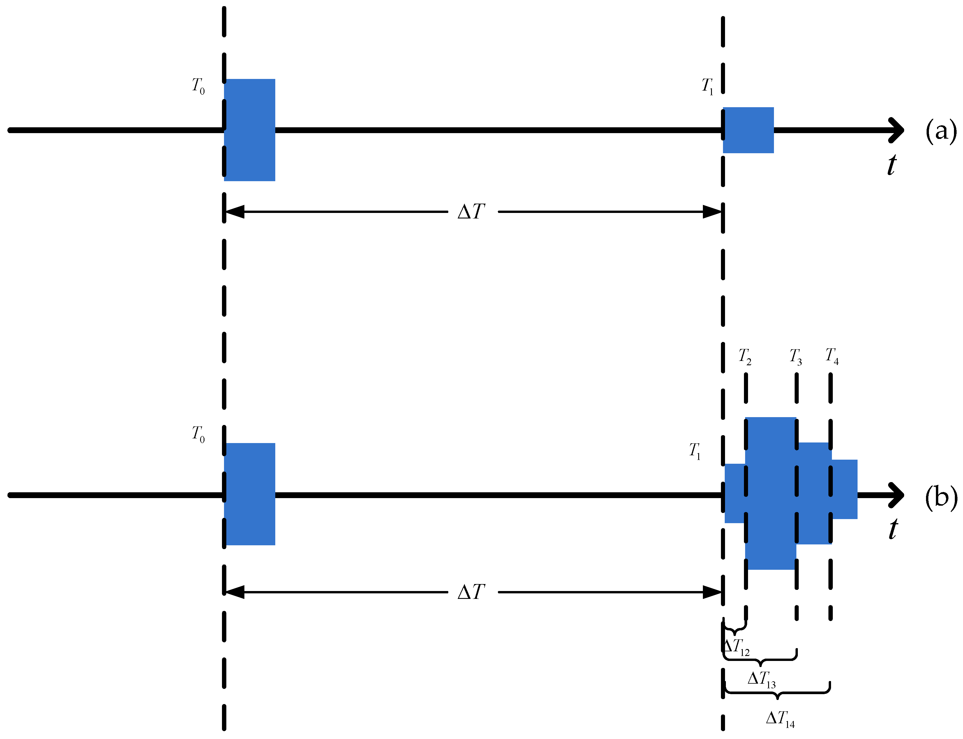
2. Problem Statement

The pulse ranging model under ideal condition is shown in Figure 1a. The ranging system emits the probe signal $s\left(t\right)$ with duration $T_s$ and records the transmitting time $T_0$. The echo signal from target is $y_{ideal}\left(t\right)$

$$y_{ideal}\left(t\right)=as(t-T_1)+v\left(t\right),$$

(1)

where a is the attenuation coefficient, $T_1$ is the direct transmitting delay, and $v\left(t\right)$ is the additive noise and is independent of $s\left(t\right)$.

For obtaining the reaching time $T_1$ of echo signal, we process $y_{ideal}\left(t\right)$ by cross-correlation. The function of cross-correlation is defined as

$$R_{x_1{x}_2}\left(\tau \right)={\int }_{-\infty }^{+\infty }{x}_1\left(t\right)x_2(t+\tau )\mathrm{d}t,$$

(2)

where $R_{x_1{x}_2}\left(\tau \right)$ is the output of cross-correlation of $x_1$ and $x_2$.

By cross-correlation, we can obtain $R_{y_{ideal}s}\left(\tau \right)$

$$\begin{array}{cc}\hfill R_{y_{ideal}s}\left(\tau \right)& ={\int }_{-\infty }^{+\infty }{y}_{ideal}\left(t\right)s(t+\tau )\mathrm{d}t\hfill \\ \hfill & =a{R}_{ss}(\tau -T_1)+R_{vs}\left(\tau \right),\hfill \\ \hfill & =a{R}_{ss}(\tau -T_1),\hfill \end{array}$$

(3)

where $R_{ss}\left(\tau \right)$ denotes the cross-correlation of emitted signal $s\left(t\right)$. Note that the noise $v\left(t\right)$ is independent of $s\left(t\right)$, $R_{vs}\left(\tau \right)=0$. This operation results in a peak in the cross-correlation spectrum. We can obtain the transmitting delay $T_1$ by searching for the position of the peak,

$$\begin{array}{cc}\hfill T_1& =\hat{\tau }\hfill \\ \hfill & =arg\underset{\tau }{max}{\left|R_{y_{ideal}s}\left(\tau \right)\right|}^2.\hfill \end{array}$$

(4)

The time delay difference $\Delta T$ between transmitting signal and target echo signal can be accurately calculated by $\Delta T=T_1-T_0$. Then, the distance R can be simply calculated by $R=(c\Delta T)/2$ with the sound speed c.

However, due to multi-path effect of UWA channel, the signal propagates along different paths, e.g., the path from surface to seabed, or the path scattered by underwater particles. Therefore, different versions of received signals corresponding to different delays and phases are superimposed at the receiver. The received signal has a fluctuated spread, as shown in Figure 1b. Assumed that the UWA channel is time-invariant in the observation time, the expression of UWA channel impulse response is

$$h\left(t\right)=\sum _{n=1}^N{a}_n\delta \left(t-T_1-\Delta T_{1n}\right),$$

(5)

where N is the total number of paths; $a_n$ is the amplitude of n-th path; $\Delta T_{1n}$ represents the delay differences between the n-th path and the direct path.

In this multi-path channel condition, the received signal $y\left(t\right)$ is

$$\begin{array}{cc}\hfill y\left(t\right)& =s\left(t\right)\ast h\left(t\right)\hfill \\ \hfill & =\sum _{n=1}^N{a}_{n}s\left(t-T_1-\Delta T_{1n}\right)+v\left(t\right),\hfill \end{array}$$

(6)

where the symbol ∗ denotes convolution.

Substituting (6) into (2) with $y\left(t\right)$ set to $x_1\left(t\right)$ and $s\left(t\right)$ set to $x_2\left(t\right)$, we can obtain $R_{ys}\left(\tau \right)$

$$\begin{array}{cc}\hfill R_{ys}\left(\tau \right)& ={\int }_{-\infty }^{+\infty }y\left(t\right)s(t+\tau )\mathrm{d}t\hfill \\ \hfill & =\sum _{n=1}^N{R}_{ss}(\tau -T_1-\Delta T_{1n}).\hfill \end{array}$$

(7)

Equation (7) indicates that $R_{ys}\left(\tau \right)$ is consist of N peaks. Some paths with similar amplitude in UWA channel make corresponding peak values close in cross-correlation spectrum. It is hardly to distinguish the direct transmitting delay between those peaks. The performance of traditional cross-correlation ranging method will be deteriorated in multi-path channel.

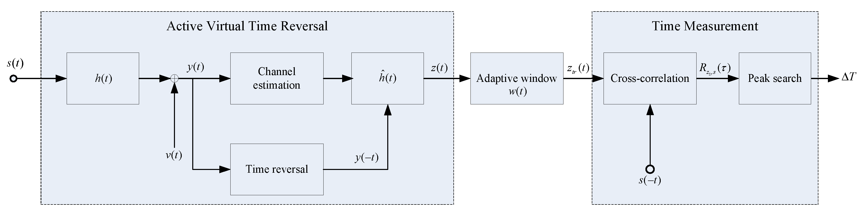
3. Active Virtual Time Reversal Based Pulse Ranging

Attracted by the focusing ability of TR, we utilize TR to improve the accuracy of time measurement and hence pulse ranging. Among current TR techniques, the active virtual time reversal model is more suitable for the pulse ranging mission. In this paper, we propose a AVTR-based pulse ranging method, the diagram of which is shown in Figure 2. The ranging model is mainly composed of three blocks, i.e., active virtual time reversal, adaptive windowing and time measurement. In the following we explain these three blocks in detail.

3.1. Active Virtual Time Reversal

The active virtual time reversal model can be divided into two phases. In phase 1, the transmitted signal $s\left(t\right)$ emitted by sonar system is passed through the UWA multi-path channel. The echo signal $y\left(t\right)$ reflected by the target is then propagated back and received by the receiver. In phase 2, the UWA channel response $\hat{h}\left(t\right)$ can be estimated from received signal $y\left(t\right)$ based on the emitted signal $s\left(t\right)$. Then the received signal $y\left(t\right)$ is time-reversed, and passes through the estimated channel $\hat{h}\left(t\right)$. We can obtain the virtual received signal denoted by $z\left(t\right)$

$$z\left(t\right)=y(-t)\ast \hat{h}\left(t\right).$$

(8)

Ideally, the estimated channel $\hat{h}\left(t\right)$ has the same amplitudes $a_n$ and delay differences $\Delta T_{1n}$ as the real channel $h\left(t\right)$. The expression of $\hat{h}\left(t\right)$ is

$$\hat{h}\left(t\right)=\sum _{n=1}^N{a}_n\delta \left(t-\Delta T_{1n}\right).$$

(9)

Substituting (9) into (8), we can obtain

$$\begin{array}{cc}\hfill z\left(t\right)& =y(-t)\ast \hat{h}\left(t\right)\hfill \\ \hfill & =\left(\sum _{n=1}^N{a}_{n}s\left(-t-T_1-\Delta T_{1n}\right)+v(-t)\right)\ast \sum _{n=1}^N{a}_n\delta \left(t-\Delta T_{1n}\right)\hfill \\ \hfill & =\sum _{n=1}^N{a}_n^{2}s(-t-T_1)+\sum _{m=1}^N\sum _{\genfrac{}{}{0pt}{}{n=1}{m\ne n}}^N{a}_m{a}_{n}s\left(-t-T_1-{\tau }_{mn}\right)+\sum _{n=1}^N{a}_{n}v\left(-t-T_1-{\tau }_n\right),\hfill \end{array}$$

(10)

where ${\tau }_{mn}={\tau }_m-{\tau }_n$ is the delay difference between the m-th path and the n-th path. We shall refer ${\tau }_{mn}$ simply as the channel delay difference in the following.

From (10) we can observe that on the right side of $z\left(t\right)$ the first term is the superposition of each multi-path signals after time delay alignment. It means the expanded signal $y\left(t\right)$ is focusing after processed by AVTR.

The performance gain of AVTR can be quantified by signal to noise gain (SNRG)

$$\mathrm{SNRG}=\frac{{\mathrm{SNR}}_{\mathrm{out}}}{{\mathrm{SNR}}_{\mathrm{in}}}.$$

(11)

In (11), ${\mathrm{SNR}}_{\mathrm{in}}$ denotes the signal to noise ratio of (6) and can be described as

$$\begin{array}{cc}\hfill {\mathrm{SNR}}_{\mathrm{in}}& =\frac{P\left[s\left(t-T_1-\Delta T_{1n}\right)\right]}{P\left[v\right(t\left)\right]}\hfill \\ \hfill & \approx \frac{a_1^2{P}_s}{P_v},\hfill \end{array}$$

(12)

where $P\left[x\right]$ denotes the power of x; $P_s$ and $P_v$ are the power of $s\left(t\right)$ and $v\left(t\right)$, respectively. ${\mathrm{SNR}}_{\mathrm{out}}$ is the signal to noise ratio of (10) and can be expressed as

$$\begin{array}{cc}\hfill {\mathrm{SNR}}_{\mathrm{out}}& =\frac{P\left[{\sum }_{n=1}^N{a}_n^{2}s(-t-T_1)\right]}{P\left[v\left(-t-T_1-{\tau }_n\right)\right]}\hfill \\ \hfill & \approx \frac{{\left({\sum }_{n=1}^N{a}_n^2\right)}^2{P}_s}{a_1^2{P}_v}.\hfill \end{array}$$

(13)

Substituting (12) and (13) into (11), we can obtain

$$\begin{array}{cc}\hfill \mathrm{SNRG}& ={\left(1+\frac{{\sum }_{n=2}^N{a}_n^2}{a_1^2}\right)}^2\hfill \\ \hfill & ⩾1.\hfill \end{array}$$

(14)

Equation (14) shows that, processed by AVTR, the ${\mathrm{SNR}}_{\mathrm{out}}$ is not less than ${\mathrm{SNR}}_{\mathrm{in}}$. This means AVTR can provide a positive gain for ranging system. The magnitude of $\mathrm{SNRG}$ depends on the type of channel impulse response. When there is no multi-path, i.e., $h\left(t\right)=a_1\delta (t-T_1)$, $\mathrm{SNRG}$ is equal to 1. When the channel impulse response is complex by rich scattering, the performance gain can be huge.

3.2. Energy-Based Adaptive Windowed Algorithm

In order to extract the focus item of the virtual time reversal received signal, we propose the energy-based adaptive windowed algorithm which can preserve the signal focus peak while maximally truncating the side peak component.

We use $z\left(n\right)$, $n=\{1,2,\cdots ,N_z\}$ to denote the discrete sequences of the time signal $z\left(t\right)$, where $N_z$ is the length of the received sequence processed by time reversal. Similarly, the discrete sequences of transmitted signal $s\left(t\right)$ is denoted by $s\left(n\right)$, $n=\{1,2,\cdots ,N_s\}$ with $N_s$ beginning the length of the emitted sequence. Apparently, the transmitted length is smaller than the received length due to time expansion and tail, i.e., $N_s<N_z$. Because time reversal has the ability of recovering the original signal [22], we expect to utilize a window function $w\left(t\right)$ whose window has the same length as the emitted sequence to localize and extract the focus part. The discrete sequences of $w\left(t\right)$ is $w\left(n\right)$

$$w\left(n\right)=\left\{\begin{array}{ccc}\hfill 1,& & N_E\le n\le N_E+N_s-1,\hfill \\ \hfill 0,& & otherwise.\hfill \end{array}\right.$$

(15)

Note that $N_E$ determines which part of the received signal will be extracted. We propose to select $N_E$ within the principle of maximizing the energy of sliding data. The method is referred to as energy-based adaptive windowed method. For a given $N_E$, the windowed signal $z_w\left(n^{\prime }\right)$ is given by

$$\begin{array}{c}\hfill z_w\left(n^{\prime }\right)=z\left(n\right)w\left(n\right),n^{\prime }=1,2,\cdots ,N_s;n=N_E,\dots ,N_E+N_s-1.\end{array}$$

(16)

We can compute the energy of the windowed signal as a function of $N_E$:

$$E\left(N_E\right)=\sum _{n^{\prime }=1}^{N_s}{\left|z_w\left(n^{\prime }\right)\right|}^2,$$

(17)

the energy-based adaptive windowed method aims to find a $N_E$ among multiple candidates which maximizes the energy:

$$arg\underset{N_E}{max}E\left(N_E\right),N_E=1:L:N_z,$$

(18)

with L the step-size which is a positive integer.

3.3. Time Measurement

Windowing the time reversed signal, we can obtain

$$\begin{array}{cc}\hfill z_w\left(t\right)& =w\left(t\right)z\left(t\right)\hfill \\ & =\underset{expectedsignal}{\underbrace{\sum _{n=1}^N{a}_n^{2}s(-t-T_1)}}+\underset{harmfulsignal}{\underbrace{w\left(t\right)\left(\sum _{m=1}^N\sum _{\genfrac{}{}{0pt}{}{n=1}{m\ne n}}^N{a}_m{a}_{n}s\left(-t-T_1-{\tau }_{mn}\right)+\sum _{n=1}^N{a}_{n}v\left(-t-T_1-{\tau }_n\right)\right)}}.\hfill \\ \hfill \end{array}$$

(19)

The right-hand side of (19) is consist of two parts. The first term is the expected signal that contains the information of time delay $T_1$ which we expect to obtain. The last term is the harmful signal which is truncated by adaptive window function.

Cross correlating (19) with $s(-t)$,

$$\begin{array}{cc}\hfill R_{z_{w}s}\left(\tau \right)& ={\int }_{-\infty }^{+\infty }{z}_w\left(t\right)s(-t-\tau )\mathrm{d}t\hfill \\ \hfill & =A{R}_{ss}(\tau -T_1)+R_{hs}\left(\tau \right),\hfill \end{array}$$

(20)

where $A={\sum }_{n=1}^N{a}_n^{2}s(-t-T_1)$, $R_{ss}$ is the autocorrelation of $s(-t)$, and $R_{hs}$ is the cross-correlation of harmful signal with $s(-t)$.

From (20) we can obtain the transmitting delay $T_1$ by searching for the position of the peak in the cross-correlation spectrum,

$$\begin{array}{cc}\hfill T_1& =\widehat{{\tau }^{\prime }}\hfill \\ \hfill & =arg\underset{{\tau }^{\prime }}{max}{\left|R_{z_{w}s}\left({\tau }^{\prime }\right)\right|}^2.\hfill \end{array}$$

(21)

4. Performance Analysis

4.1. Simulation Analysis

Simulations have been carried out to demonstrate the effectiveness of time reversal based pulse ranging method. The simulation conditions are as follows.

(1)

Linear frequency modulation (LFM) signal is employed as the emitted signal shown in Figure 3, the frequency range is 10 to 12 kHz, and the signal time width is 20 ms.

(2)

The underwater acoustic channel is generated by Bellhop hydroacoustic toolbox [32]. For the convenience of calculation, the equal sound velocity gradient is used as the environmental input parameter of Bellhop in the simulation. The simulation parameters and applied values are given in

Table 1. Sound field environment parameter.

Parameter Name	Numerical Value
Average sound speed	1505 m/s
Water depth	90 m
Source depth	50 m
Receiver depth	50 m
Range	1000 m

.

The main parameters of acoustic channel generated by Bellhop are reported in

Table 2. Acoustic channel parameter. Blackbody numbers represent direct path parameters.

Amplitude	Delay (ms)	Number of Sea Surface Reflections	Number of Seafloor Reflections
$1.916\times {10}^{-4}$	733.8	3	2
$5.281\times {10}^{-4}$	708.6	2	2
$8.288\times {10}^{-4}$	692.3	2	1
$9.550\times {10}^{-4}$	670	1	0
$9.950\times {10}^{-4}$	666.7	0	0
$9.510\times {10}^{-4}$	668.8	0	1
$8.950\times {10}^{-4}$	677.4	1	1
$1.099\times {10}^{-4}$	728.3	1	2

. The generated simulation channel is depicted in Figure 4.

The time domain waveform of the received signal after the detection signal passing through the simulation channel is shown in Figure 5. The red line represents the windowed received signal, and the blue line represents the unwindowed received signal. The signal shown in Figure 6 represents the output of the received signal cross-correlated with the emitted signal. The red line represents the windowed output signal and the blue line represents the unwindowed output signal. From Figure 5 and Figure 6, we can find that due to the multipath effect, the emitted signal passing through the simulation channel will be time-expanded. The cross-correlation output of the received signal will have multiple sharp peaks, and the real arrival time is difficult to extract. The simulation results show that in the multipath environment of shallow water, the cross-correlation output of the received signal will have pseudo-peaks, which will affect the accuracy of the time measurement that has a huge impact on ranging. The simulation result is consistent with the above theoretical analysis.

The processing method shown in Figure 2 is performed on the received signal, and the output results are shown in Figure 7 and Figure 8. The red line represents the windowed output signal and the blue line represents the unwindowed output signal. According to Figure 7, we can find that the received signal which is processed by AVTR are superimposed in the same position to achieve energy focusing. The signal after windowing can further suppress the energy of the side lobes in Figure 8. The simulation results show that compared with the traditional ranging method, the time-reversed-based ranging method proposed in this paper has better ranging performance.

We compare the performance of AVTR based pulse ranging method and cross-correlation ranging methods. For cross-correlation we used the first peak detection algorithm and the highest peak detection algorithm. The mean distance shown in Figure 9 and root mean square error (RMSE) shown in Figure 10 are computed by averaging over 1000 Monte Carlo simulations at different signal-to-noise ratio (SNR). It is confirmed that, due to the influence of multi-path, when ranging by cross-correlation method, the peak value corresponding to the cross-correlation output may not be the direct path. This phenomenon produces a bias for cross-correlation ranging method. While the proposed ranging method in this paper can eliminate the bias generated by multipath. The proposed method has a better performance compared to cross-correlation method.

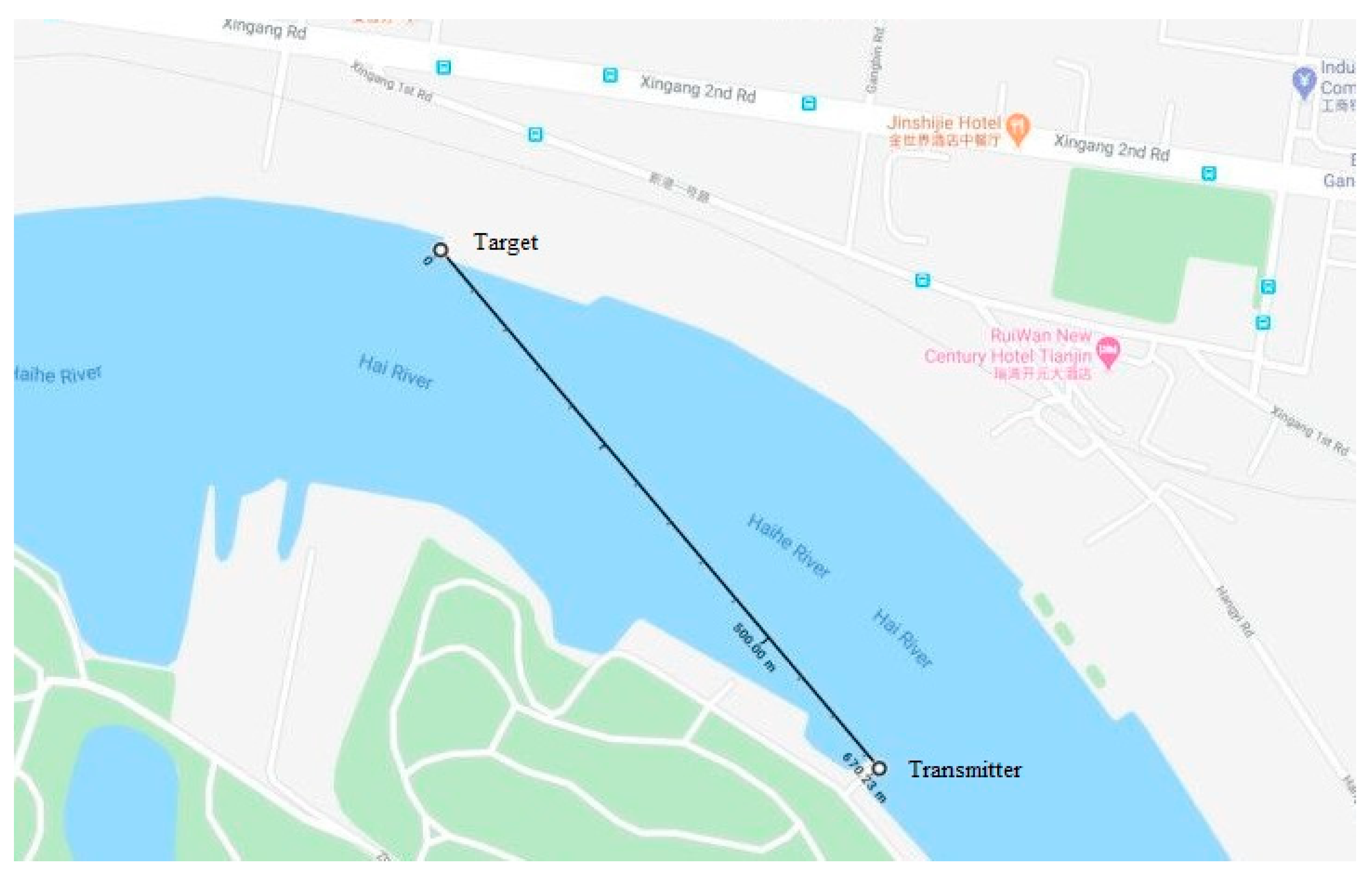
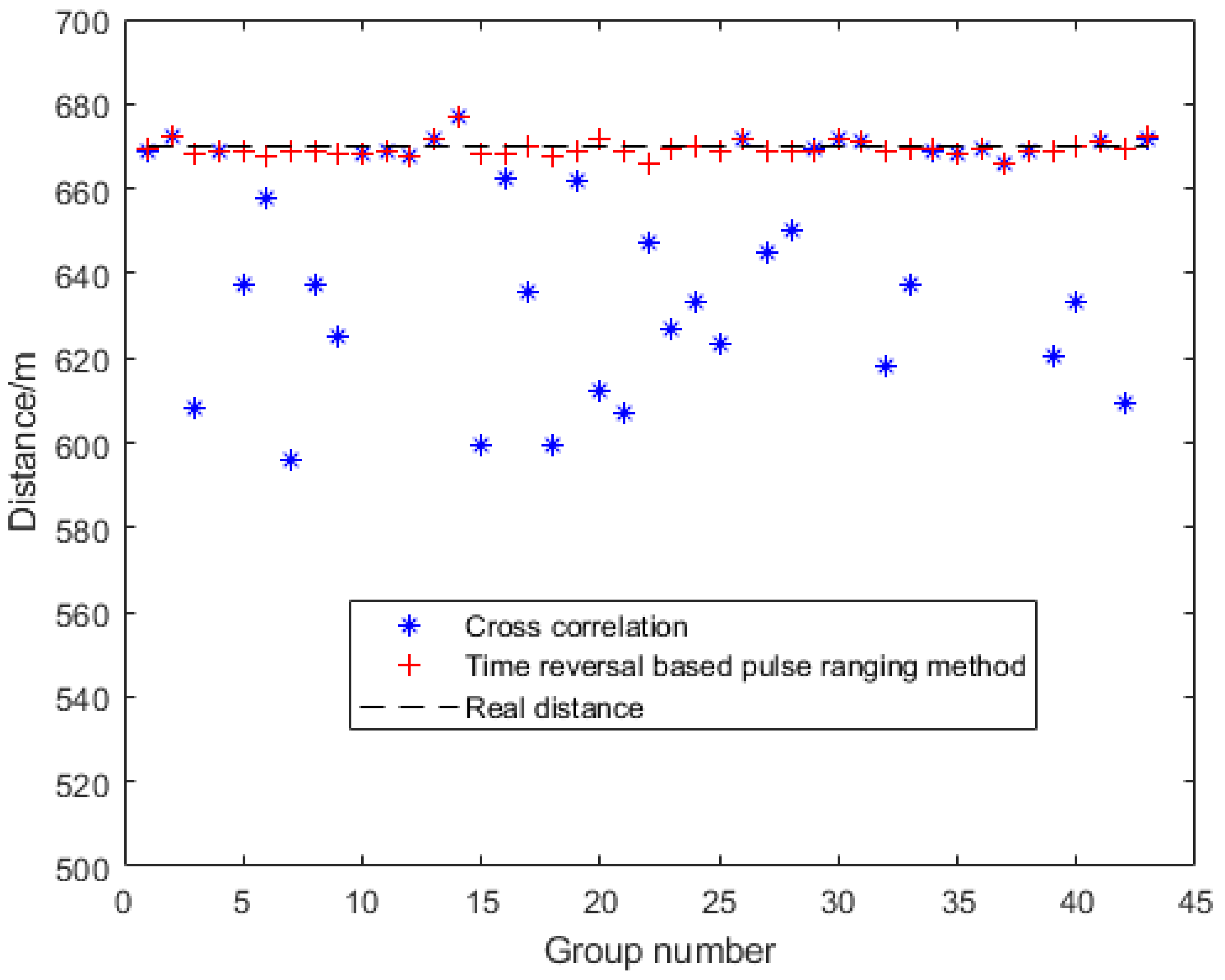
4.2. Experimental Analysis

On 17 October 2018, the pulse-ranging method experiment based on AVTR was carried out in Tanggu Haihe, Binhai New Area of Tianjin. The water depth of the experimental water is about 10 m, and the sound velocity gradient is shown in Figure 11. The experimental vessels are 670 m apart, and the water depth of the sensor and target is 4 m. The location of transmitter and target is illustrating in Figure 12. We put a icListen smart hydrophone near the transmitter. It can record both the transmitted signal and the echo signal. To get the echo signal, we use a transceiver as a virtual target instead of the real target. The transceiver received the emitted signal. We calculated the source level of the virtual target through sonar equation. The amplification factor was determined by the source level of the virtual target. Then the virtual target sent back the amplified signal. The frequency of transmitted LFM signal is 10–13 kHz. The transmitted signal is 0.1 s.

We acquire and display 43 sets of data, as shown in Figure 13. Here, we show the estimated channel impulse response of the first set of data in Figure 14. The experimental data are analyzed by cross-correlation ranging method and the proposed method in this paper, respectively. The results are shown in Figure 15. The RMSE of the two ranging methods are calculated by the obtained 43 sets of data separately, and the results are shown in

Table 3. RMSE of two ranging methods.

Method	RMSE (m)
Cross correlation ranging	34.3
Time reversal based pulse ranging	2.0

.

Figure 15 shows that the measurement result of the proposed ranging method is stable around 670 m, which is robust compared to the cross-correlation method. These two kinds of pulse ranging results have a bias with GPS. There are two reasons for this phenomenon: One is the measurement error of the GPS itself, and the other is that we choose average sound speed as the input parameter when measuring, while the sound speed in the outfield environment that is shown in Figure 11 is not constant. The RMSE of the cross-correlation ranging method is 34.3 m, and the RMSE of the pulse ranging method based on time reversal in this paper is 2.0 m. The experimental results indicate that the proposed ranging method in this paper has a better ranging performance than the cross-correlation ranging method.

5. Conclusions

The pulse ranging method is a commonly used method for underwater ranging. However, due to the complexity of the underwater acoustic environment, multi-path channel will have a negative impact on the ranging results and reduce the accuracy of ranging. In this paper, a active virtual time reversal pulse ranging method has been proposed to improve the ranging accuracy by using the focusing characteristics of time reversal. Compared with the traditional cross-correlation ranging method, the proposed algorithm can make the receiving signal focus on the receiving end, eliminate the interference of multiple pseudo-peaks, and improve the measurement accuracy. Simulation and experimental results validated the effectiveness of the proposed method.

References

1. Zou, Z.G.; Xu, X.M.; Tao, Y.; Zhu, Z.T. Joint Design of Ranging and Media Access Control in Underwater Acoustic Networks. In Advanced Materials Research; Trans Tech Publications Ltd.: Stafa-Zurich, Switzerland, 2012; Volume 546, pp. 1261–1269. [Google Scholar]
2. Wang, J.; Park, J.G. A Novel Indoor Ranging Algorithm Based on a Received Signal Strength Indicator and Channel State Information Using an Extended Kalman Filter. Appl. Sci. 2020, 10, 3687. [Google Scholar] [CrossRef]
3. Liu, J.C.; Cheng, Y.T.; Hung, H.S. Joint bearing and range estimation of multiple objects from time-frequency analysis. Sensors 2018, 18, 291. [Google Scholar] [CrossRef] [PubMed] [Green Version]
4. Yangmei, Z.; Weijie, T. Underwater segmented sparse decomposition ranging method. In Proceedings of the 2015 IEEE International Conference on Signal Processing, Communications and Computing (ICSPCC), Ningbo, China, 19–22 September 2015; pp. 1–4. [Google Scholar]
5. Bayat, M.; Crasta, N.; Aguiar, A.P.; Pascoal, A.M. Range-based underwater vehicle localization in the presence of unknown ocean currents: Theory and experiments. IEEE Trans. Control Syst. Technol. 2015, 24, 122–139. [Google Scholar] [CrossRef]
6. Xia, Z.; Li, X.; Meng, X. High resolution time-delay estimation of underwater target geometric scattering. Appl. Acoust. 2016, 114, 111–117. [Google Scholar] [CrossRef]
7. Shatara, S.; Tan, X. An efficient, time-of-flight-based underwater acoustic ranging system for small robotic fish. IEEE J. Ocean. Eng. 2010, 35, 837–846. [Google Scholar] [CrossRef]
8. Kay, S.M. Fundamentals of Statistical Signal Processing; Prentice Hall PTR: Upper Saddle River, NJ, USA, 1993. [Google Scholar]
9. Wang, D.; Fattouche, M. OFDM transmission for time-based range estimation. IEEE Signal Process. Lett. 2010, 17, 571–574. [Google Scholar]
10. Win, M.Z.; Scholtz, R.A. Characterization of ultra-wide bandwidth wireless indoor channels: A communication-theoretic view. IEEE J. Sel. Areas Commun. 2002, 20, 1613–1627. [Google Scholar] [CrossRef] [Green Version]
11. Giorgetti, A.; Chiani, M. Time-of-arrival estimation based on information theoretic criteria. IEEE Trans. Signal Process. 2013, 61, 1869–1879. [Google Scholar] [CrossRef]
12. Song, S.; Zhang, Q. Multi-dimensional detector for UWB ranging systems in dense multipath environments. IEEE Trans. Wirel. Commun. 2008, 7, 175–183. [Google Scholar] [CrossRef]
13. Braasch, M. Multipath Effects, Global Positioning Systems: Theory and Applications; American Institute of Aeronautics and Astronautics: Reston, VA, USA, 1996; Chapter 14; Volume 1. [Google Scholar]
14. Freeman, S.E.; Emokpae, L.; Nicholas, M.; Edelmann, G.F. A highly directional transducer for multipath mitigation in high-frequency underwater acoustic communications. J. Acoust. Soc. Am. 2015, 138, EL151–EL154. [Google Scholar] [CrossRef] [Green Version]
15. Zeng, W.J.; Jiang, X.; Li, X.L.; Zhang, X.D. Deconvolution of sparse underwater acoustic multipath channel with a large time-delay spread. J. Acoust. Soc. Am. 2010, 127, 909–919. [Google Scholar] [CrossRef]
16. Li, C.X.; Guo, M.F.; Zhao, H.F. An Iterative Deconvolution-Time Reversal Method with Noise Reduction, a High Resolution and Sidelobe Suppression for Active Sonar in Shallow Water Environments. Sensors 2020, 20, 2844. [Google Scholar] [CrossRef]
17. On, B.; Im, S.; Seo, I. Performance of Time Reversal Based Underwater Target Detection in Shallow Water. Appl. Sci. 2017, 7, 1180. [Google Scholar] [CrossRef] [Green Version]
18. Fink, M. Time reversal of ultrasonic fields. I. Basic principles. IEEE Trans. Ultrason. Ferroelectr. Freq. Control 1992, 39, 555–566. [Google Scholar] [CrossRef]
19. Prada, C.; Manneville, S.; Spoliansky, D.; Fink, M. Decomposition of the time reversal operator: Detection and selective focusing on two scatterers. J. Acoust. Soc. Am. 1996, 99, 2067–2076. [Google Scholar] [CrossRef]
20. Kuperman, W.; Hodgkiss, W.S.; Song, H.C.; Akal, T.; Ferla, C.; Jackson, D.R. Phase conjugation in the ocean: Experimental demonstration of an acoustic time-reversal mirror. J. Acoust. Soc. Am. 1998, 103, 25–40. [Google Scholar] [CrossRef] [Green Version]
21. Sabra, K.G.; Roux, P.; Song, H.C.; Hodgkiss, W.; Kuperman, W.A.; Akal, T.; Stevenson, M.R. Experimental demonstration of time-reversed reverberation focusing in a rough waveguide. Application to target detection. J. Acoust. Soc. Am. 2005, 118, 1904. [Google Scholar] [CrossRef]
22. Moura, J.M.; Jin, Y. Detection by time reversal: Single antenna. IEEE Trans. Signal Process. 2006, 55, 187–201. [Google Scholar] [CrossRef]
23. Pan, X.; Li, C.; Xu, Y.; Xu, W.; Gong, X. Combination of time-reversal focusing and nulling for detection of small targets in strong reverberation environments. IET Radar Sonar Navig. 2014, 8, 9–16. [Google Scholar] [CrossRef]
24. Song, H.C. An overview of underwater time-reversal communication. IEEE J. Ocean. Eng. 2015, 41, 644–655. [Google Scholar] [CrossRef]
25. Lei, W.; Yao, L. Performance Analysis of Time Reversal Communication Systems. IEEE Commun. Lett. 2019, 23, 680–683. [Google Scholar] [CrossRef]
26. Ciuonzo, D.; Romano, G.; Solimene, R. Performance analysis of time-reversal MUSIC. IEEE Trans. Signal Process. 2015, 63, 2650–2662. [Google Scholar] [CrossRef]
27. Xu, Q.; Safar, Z.; Han, Y.; Wang, B.; Liu, K.R. Statistical learning over time-reversal space for indoor monitoring system. IEEE Internet Things J. 2018, 5, 970–983. [Google Scholar] [CrossRef]
28. Huang, P.; Xia, X.G.; Liu, X.; Liao, G. Refocusing and motion parameter estimation for ground moving targets based on improved axis rotation-time reversal transform. IEEE Trans. Comput. Imaging 2018, 4, 479–494. [Google Scholar] [CrossRef]
29. Foroozan, F.; Asif, A. Time reversal based active array source localization. IEEE Trans. Signal Process. 2011, 59, 2655–2668. [Google Scholar] [CrossRef] [Green Version]
30. Yang, F.-Z.; Wang, H.-Y.; Shen, X.-H.; Ning, W.-Z. The performance of time reversal passive detection over underwater multi-path channel. In Proceedings of the 2011 IEEE International Conference on Signal Processing, Communications and Computing (ICSPCC), Xi’an, China, 14–16 September 2011; pp. 1–4. [Google Scholar]
31. Jing, H.; Wang, H.; Liu, Z.; Shen, X. DOA estimation for underwater target by active detection on virtual time reversal using a uniform linear array. Sensors 2018, 18, 2458. [Google Scholar] [CrossRef] [Green Version]
32. Jensen, F.B.; Kuperman, W.A.; Porter, M.B.; Schmidt, H. Computational Ocean Acoustics; Springer Science & Business Media: Berlin, Germany, 2011. [Google Scholar]
Figure 1. Pulse ranging model under different conditions. (a) Pulse ranging model under ideal condition. (b) Pulse ranging model under multi-path condition.
Jmse 08 00883 g001
Figure 2. Diagram of TR-based pulse ranging.
Jmse 08 00883 g002
Figure 3. Emitted linear frequency modulation (LFM) signal.
Jmse 08 00883 g003
Figure 4. Simulated channel by bellhop.
Jmse 08 00883 g004
Figure 5. Target echo signal in time domain.
Jmse 08 00883 g005
Figure 6. Output of the received signal cross-correlated with the emitted signal before active virtual time reversal.
Jmse 08 00883 g006
Figure 7. Target echo signal in time domain after active virtual time reversal.
Jmse 08 00883 g007
Figure 8. Output of the received signal cross-correlated with the emitted signal after active virtual time reversal.
Jmse 08 00883 g008
Figure 9. Mean distance of each ranging methods under different signal-to-noise ratios (SNRs).
Jmse 08 00883 g009
Figure 10. Root mean square error (RMSE) of each ranging methods under different SNRs.
Jmse 08 00883 g010
Figure 11. Sound speed profile.
Jmse 08 00883 g011
Figure 12. Illustrative diagram for ranging experiment environment.
Jmse 08 00883 g012
Figure 13. The waveform of recorded signal by IcListen Smart Hydrophone.
Jmse 08 00883 g013
Figure 14. The estimated channel impulse response from set 1.
Jmse 08 00883 g014
Figure 15. Comparison of two methods ranging results.
Jmse 08 00883 g015