Numerical Study on Spatio-Temporal Distribution of Cold Front-Induced Waves along the Southeastern Coast of China

Abstract

Cold fronts, as one of the most frequent extreme weather events, can induce significant waves on the sea. This work analyzes the spatial and temporal variations in cold front events, especially the characteristics of wind directions during cold fronts in the East China Sea (ECS). The SWAN (Simulating Waves Nearshore) model is applied to simulating the waves induced by cold fronts. To calibrate the model, two typical cold front events were selected to simulate the corresponding waves in the ECS. The results indicate that the data misfit between the observed and modeled significant wave heights (SWH) is within a reasonable range. Idealized sensitivity experiments were then designed in order to analyze and discuss the responses of ocean waves to wind direction, swell distribution, maximum of significant wave heights (MSWH), and time lag during the cold fronts. The results show that the average MSWH in the ECS decreases monotonically with the deflection of wind direction from north-east to north-west, while specific nearshore sites do not conform to this pattern due to topography. The time series of SWH indicate that the action of the swells leads to a prolongation of the duration of catastrophic waves. This work investigates the temporal and spatial distribution characteristics of cold front-induced wind wave fields in offshore Zhejiang, which has important value for the study of the impact of cold fronts on the ocean as well as disaster prevention and mitigation efforts.

1. Introduction

In China, a cold front, which is defined when the regional averaged temperature drops more than 10 °C and the lowest temperature drops below 5 °C within one or two days, can cause strong winds [1]. The wind directions are mainly northerly and the wind speeds are generally 5–6 Beaufort. During the strong activity of cold air or the development of low pressure on land, the wind speed of a cold front gale can reach up to 7–8 Beaufort. Low temperatures aroused by cold fronts are the main cause of natural disasters, and the precipitation brought by cold fronts does great harm to agriculture. On the ocean, cold fronts can induce storm surges and large waves which have a significant negative impact on shipping, aquaculture, and coastal construction. For instance, based on 30 years of water-level hindcast data on the southeast coast of Mexico, Rey et al. [2] pointed out that cold fronts were one of the most important causes of floods in this area, and that the superposition of cold fronts and tides can cause more serious disasters. Bevington et al. [3] indicated that cold fronts reduce the land construction capacity of the delta. Huang and Li [4] found that while cold fronts had shorter influencing periods than hurricanes, the occurrence frequency of cold fronts was higher, an important factor leading to frequent exchanges between the bay and the coastal ocean. In recent years, several works have studied the variations in wind waves caused by cold fronts under the effect of climate change. For example, Appendini et al. [5] pointed out that severe wind and waves caused by cold fronts in the Gulf of Mexico would be reduced in a warming climate. In addition, most research on cold fronts has focused on extremely low temperatures, frosts, and intensive northerly winds [6,7,8,9]. These studies on cold fronts also focused on the typical cold front processes in the 1950s and 1960s [10], including their mechanisms, forecasting methods, and analysis of their characteristics [11].

For the ocean, Hsueh and Romea [12] found that the sea level in the Northeast China Sea rises during cold fronts, thus affecting human life and maritime transportation. Ortiz-royero et al. [13] analyzed the reports of Instituto de Hidrología and other institutions over the past 16 years, and summarized the time distribution of cold fronts. Their analysis results determined that cold fronts were closely related to waves in the Colombian Caribbean. Currents and waves during cold fronts have been the focus of research in recent years. Using three different methods, Payandeh et al. [14] studied the variation in currents and water levels in Barataria Bay during the cold front season. Based on velocity time-series data obtained by ADCP (acoustic Doppler current profiler), Li et al. [15] found that cold fronts had an important impact on Barataria Bay and proposed a prediction method for cold fronts. Similarly, Weeks et al. [16] used an unmanned boat and a manned boat to measure flow velocity profiles and estimated cold front-induced fluxes in the northern Gulf of Mexico. Huang and Li [17] combined ADCP observations and the Finite Volume Coastal Ocean Model (FVCOM) to study the exchange of water between Lake Pontchartrain Estuary and the coastal ocean during cold front events. In addition, Li et al. [18] used satellite images to analyze the distribution and variation of total suspended sediment concentration in the northern Gulf of Mexico during the entire process of cold fronts. Cao et al. [19] investigated the effects of two types of cold fronts on waves along coastal Louisiana based on in situ data from two offshore stations.

The East China Sea (ECS) is frequently affected by cold fronts. The impact of cold fronts in the ECS has also been studied. For instance, Mo et al. [20] simulated the wind waves generated by cold fronts in the ECS by using the Simulating Waves Nearshore (SWAN) model to reanalyze the growth of frequency spectra and the spectral parameters of wind waves, and proved the correctness of the simulation results. Li et al. [21] developed a new criterion of cold front storm surge intensity. Mo et al. [22] studied the storm surges induced by cold fronts in the Northern ECS using a numerical model, ROMS, and discussed the effects of several influencing factors on storm surges. Zhao and Jiang [23] constructed different ideal cold fronts by considering different major tracks, pressure fields, and high wind periods, and investigated their influence on the surges in the Bohai Sea using FVCOM.

In the ECS, strong waves are frequent and can significantly influence marine activities. Most studies have focused on typhoon waves; however, cold fronts can also generate strong waves, which can cause large disasters for human life, maritime transportation, etc. This has attracted the attention of some scholars. Zheng et al. [24] used the SWAN model to simulate the wave field in the Bohai Sea during a cold front process. Zhou and Xu [25] studied the characteristics of wave fields under the influence of a cold front in the sea off Jiangsu Province by using SWAN. In general, most of the previous studies have focused on simulating wave fields during a specific cold front event without further discussing the effect of the structure of cold fronts on wave fields in the ECS, which motivates this work. The numerical model is an effective method for studying wave distribution. New algorithms have been proposed in recent years, such as the numerical model developed by Borkowski [26]. In this paper, a numerical wave model, SWAN, was applied in order to simulate the wave field forced by cold fronts under different predominant wind directions. The purpose is to investigate the temporal and spatial distribution characteristics of cold-front-induced wind wave fields and swell fields along the southeastern coast of China under different wind directions, which can provide more information on ocean waves in the study area.

This paper is organized as follows: Section 2 describes the data and methodology in this study. In Section 3, two historical cold front events in Zhejiang are simulated to verify the reliability of the model, and the spatial and temporal distribution of the wave field is briefly analyzed. The same section gives a brief introduction to the major characteristics of cold fronts in China, the monthly distribution of cold front days, the frequency distribution of wind direction, and the distribution of wind speed. Finally, an experimental design and its results are given. In Section 4, the experimental results are further processed and the effects of the wind direction of a cold front on both the wave field and the swell field in offshore Zhejiang are discussed. Section 5 summarizes and concludes this work.

2. Materials and Methods

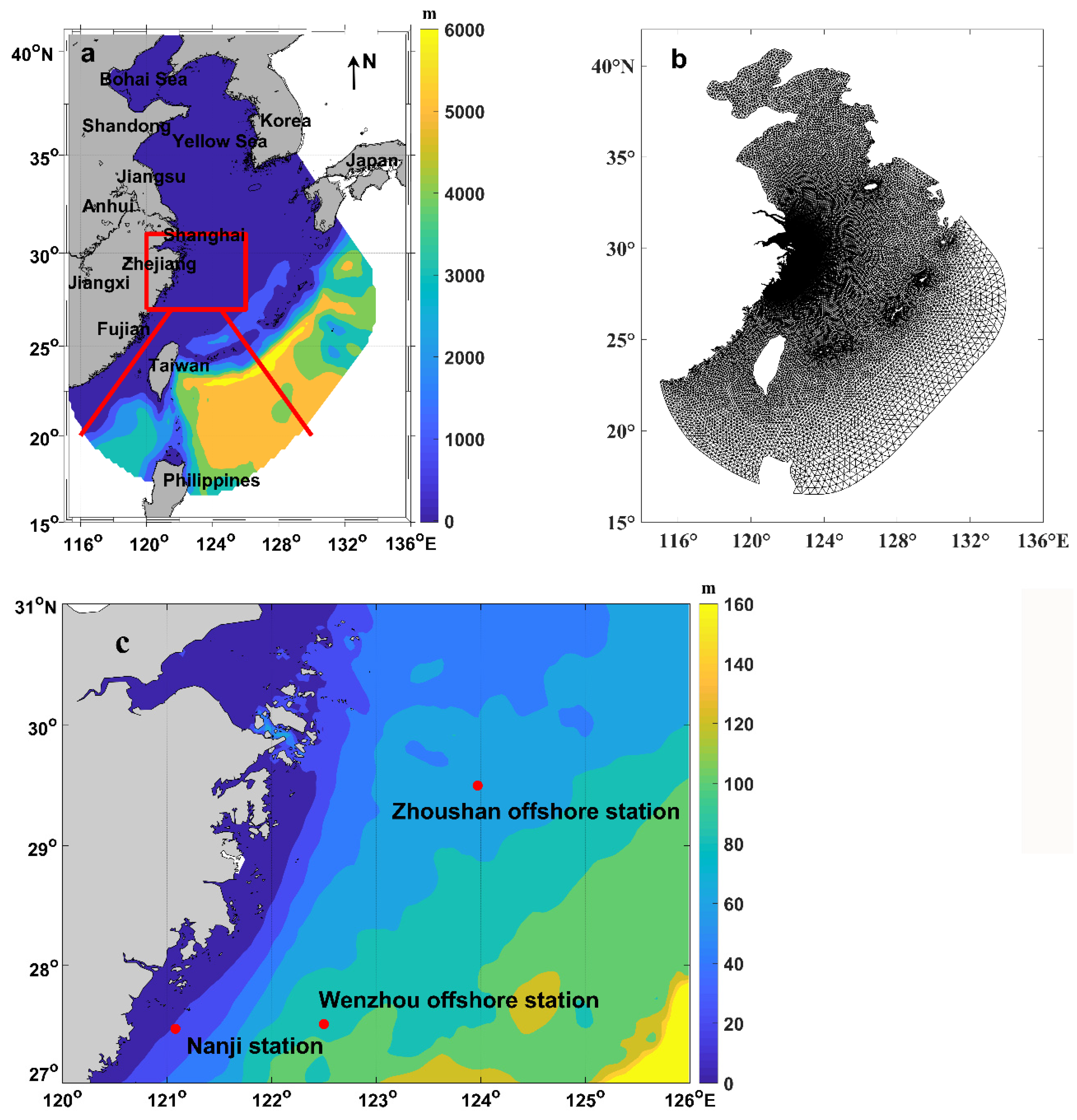
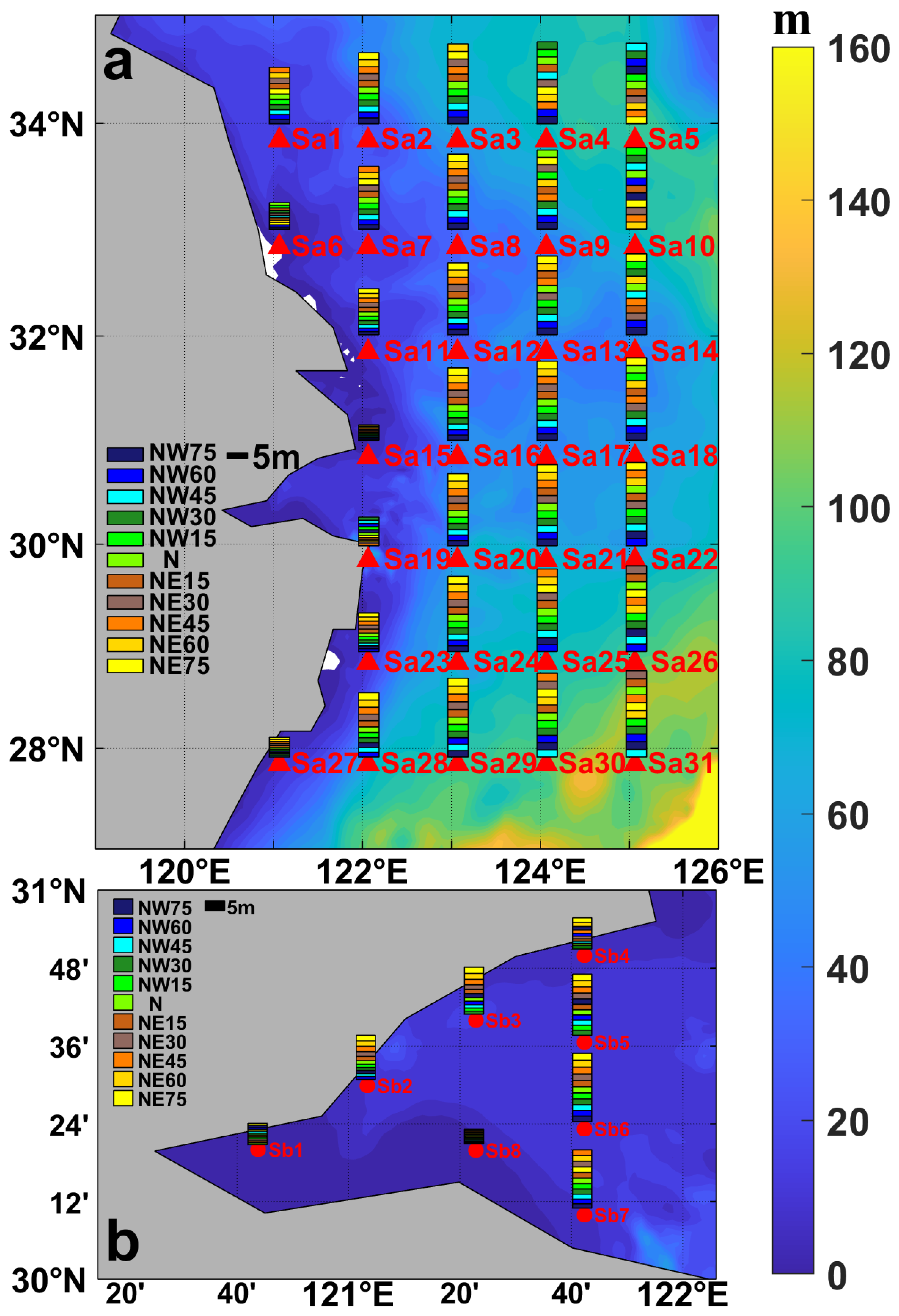
2.1. In Situ Observations

The significant wave height (SWH) observations were collected at three coastal oceanic stations: Nanji station (NJ), Wenzhou offshore station (WZ), and Zhoushan offshore station (ZS). The locations are shown in Figure 1c and the specific information pertaining to the observation sites is listed in

Table 1. Observation Site Information.

Station	Longitude	Latitude	Water Depth (m)
NJ	121.08° E	27.46° N	21.26
WZ	122.50° E	27.50° N	91.44
ZS	123.97° E	29.50° N	69.44

.

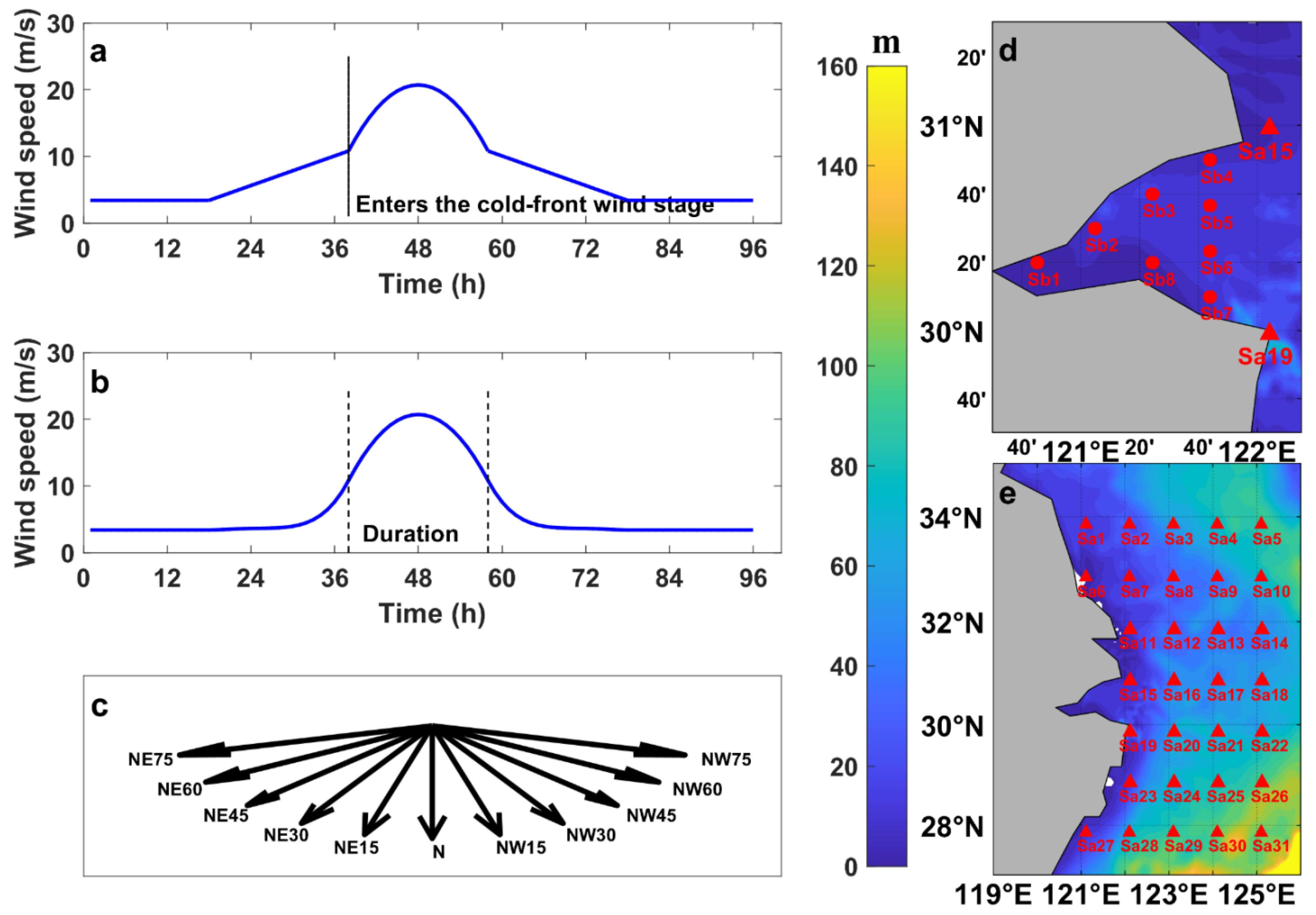
2.2. Wind Forcing Data

The CCMP (Cross-Calibrated Multi-Platform) wind field was used as the wind forcing dataset. Altas [27] confirmed that the CCMP wind field could substantially improve accuracy compared with other wind datasets measured by a single satellite platform. The time interval of the CCMP wind field is 6 h. The CCMP wind field works well with the SWAN model, and has been validated in previous works [28,29].

2.3. SWAN Model

2.3.1. Model Description

To study the spatial and temporal distribution of waves in Zhejiang offshore during cold fronts, a third-generation wave model developed by the Delft University of Technology, SWAN, was used in this study. Based on the action density balance equation and the linear stochastic surface gravity wave theory (including the action of the flow), the action density balance equation is shown below:

$$\frac{\partial }{\partial t}N+\frac{\partial }{\partial x}{C}_{x}N+\frac{\partial }{\partial y}{C}_{y}N+\frac{\partial }{\partial \sigma }{C}_{\sigma }N+\frac{\partial }{\partial \theta }{C}_{\theta }N=\frac{S}{\sigma }$$

(1)

The first term on the left side of the equation represents the rate of change of the action density with time. The second and third terms represent the propagation of the action density in geometric space; coefficients C_x and C_y are the rates of change. The fourth term indicates refraction and shallowing caused by the changes in flow and water depth. The fifth term represents the frequency shift caused by the flow and the shallowing of the water depth. S on the right side of the equation denotes the energy source term. S consists of five parts, where S_in represents wave growth by wind, S_nl3 and S_nl4 denote nonlinear wave–wave interactions, and S_ds,w, S_ds,b and S_ds,br represent wave energy dissipation caused by the white capping, bottom friction, and depth-induced wave breaking.

S = S_in + S_nl3 + S_nl4 + S_ds,w + S_ds,b + S_ds,br

(2)

N in this equation is the action density, and σ is the relative frequency. The relationship between the two physical quantities is shown in the following equation:

N = E/σ

(3)

In the SWAN model, different options are provided for each physical process. The main physical processes considered in SWAN are wind input and white capping, bottom friction, and depth-induced wave breaking. In the third-generation model, the default choice of wind input and white capping processes is KOMEN. The default option of bottom friction is the empirical JONSWAP formulation with a default constant value of friction coefficient of 0.067. The depth-induced wave breaking adopts Battjes and Janssen’s formulation in the SWAN model, which was controlled by two adjustable parameters [30].

The physical processes under shallow water are widely considered in SWAN. The SWAN model has limitations in some physical processes; for instance, it does not calculate wave-induced currents or correctly calculate diffraction in harbours or in front of reflecting obstacles. Despite this, SWAN has been widely used for numerical simulation and prediction of waves in coastal areas, lakes, etc. [31,32]. SWAN can effectively simulate the spatial and temporal characteristics of waves. The theoretical and numerical background of SWAN can be found in Holthuijsen et al. [30], Ris et al. [33], Booij et al. [34], and Zijlema and Van der Westhuysen [35].

2.3.2. Model Domain and Bathymetry

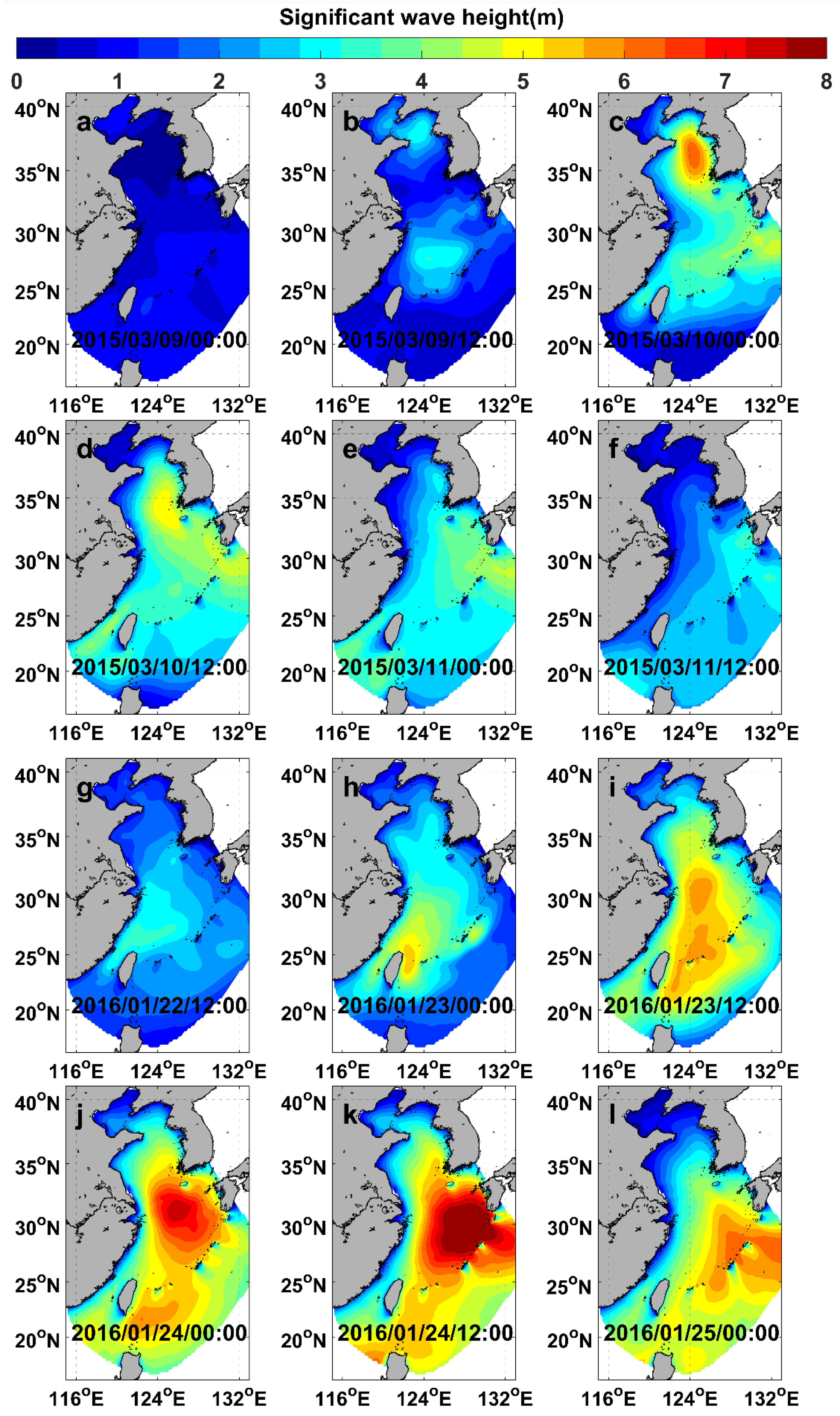
The study area here was the East China Sea, 11–43° N, 114–134° E, with a maximum water depth of about 6000 m (Figure 1a). The high-resolution bathymetry data for the coastal areas adjacent to Zhejiang province were provided by the Ocean and Fisheries Bureau of Zhejiang Province, and the data for the other areas were obtained from the ETOPO-1 (http://www.ngdc.noaa.gov/mgg/global/global.html (accessed on 15 August 2018)) dataset. As shown in Figure 1b, the unstructured triangular grid was used as the model’s computing grid. The model domain consists of 29,193 triangular elements and 15,423 nodes, and the spatial resolution gradually declines from 50 km for the open boundary to less than 1 km for the coastal zone [36].

3. Results

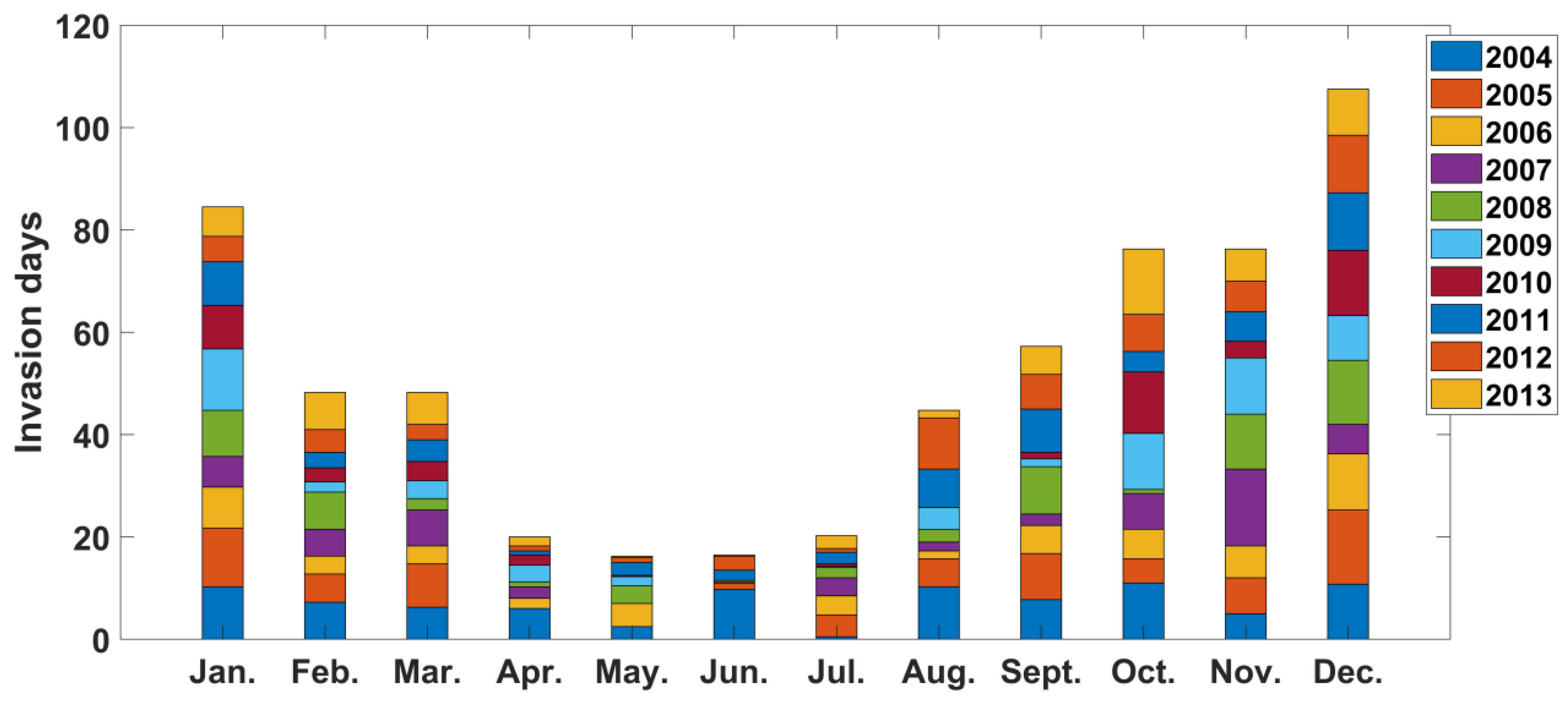
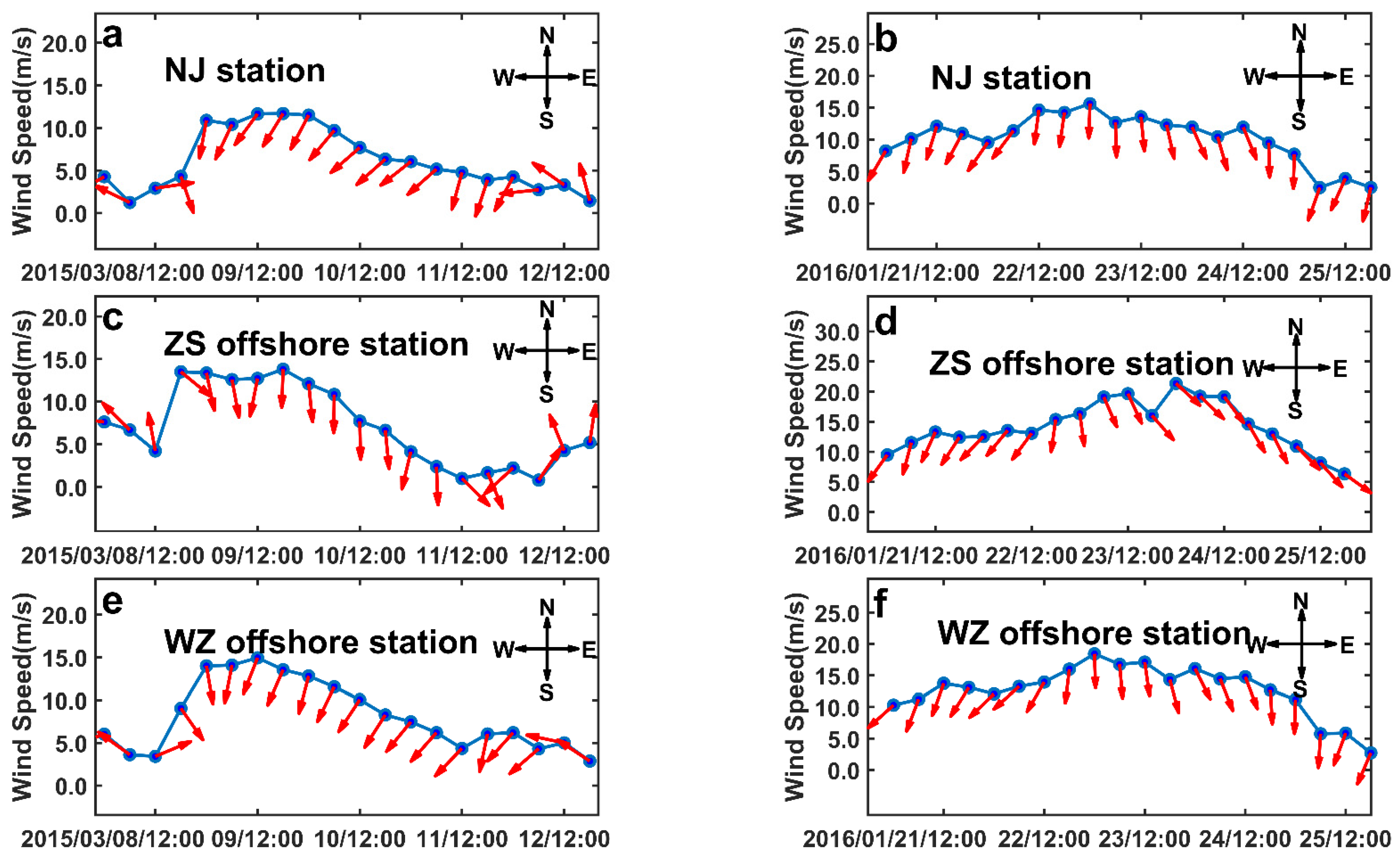
3.1. Characteristics of Wind Field during Cold Fronts

The invasion track is one of the important features of cold fronts. Previous studies have shown that cold air outbreaks mainly attack China through three paths [37]. The first, from the adjacent waters west of Novaya Zemlya, was called the northwest track, which accounted for 44% of the total number of paths. The second track was the western track from the sea south of Iceland; about 33% of the tracks were of this type. The third track, the north track, is from the ocean east of Novaya Zemlya. This track accounted for 18% of all the paths [37]. According to the historical records, more than ten cold fronts invaded China every winter [23].

In this section, we conduct a statistical analysis to better understand the cold front wind field in the ECS. Although cold fronts are defined according to cooling rates and minimum temperatures, our study focuses on wind speed enhancement and wind direction changes induced by cold fronts. In previous studies, the invasion of a strong cold front was gradually accompanied by strong winds exceeding Beaufort 6 (10.8–13.8 m/s) or 8 scale (17.2–20.7 m/s) [38].

Based on the CCMP wind field data, we took 17.2 m/s (minimum value of Beaufort 8 scale) as the threshold of the strong north wind and counted the invasion days of the north wind in different months from 2004 to 2013 [38]. Figure 2 shows that there were almost 616 days (approximately 16.86% of the total number of days) when the ECS was under strong north winds during the decade, about 62 days a year, and about 5 days a month on average. The ECS was mainly affected by the strong north wind in January, February, March, September, October, November, and December, accounting for about 90% of the total. From April to July, the north winds affecting the ECS were relatively small, accounting for only 11.9%.

According to the observation records of the Xiaoping Island meteorological station (38.48° N, 121.29° E) located in the Bohai Sea; the monthly distribution of strong north winds generally conforms to the statistic from CCMP data [39]. It should be pointed out that the north wind is not necessarily the cold front wind; however, the cold front wind belongs to the northward wind in China. Thus, the statistical characteristics of the northward wind can reveal the months in which the cold front wind concentrates. In the upcoming section, we will study the cold front wind direction and wind speed of the cold front, focusing on the period from August to March.

To clarify the main direction of the cold front wind in the ECS, 12-point windrose charts were drawn from August to April (with April as the control group) to reveal the frequency of the average north wind direction. Each concentric circle represents an occurrence frequency, increasing from the center to the perimeter. Different bands indicate the ranges of wind speeds. Except for August, northeast winds prevail in the remaining months, and northwest winds occasionally occur. Figure 3 shows that the frequency of the northeast wind gradually increased from September to December and decreased from January to April. By analyzing the meteorological data in the northern ECS from 1991 to 2000, Zhang [39] concluded that a cold front along the northwest track was accompanied by winds varying from N (north) to NNE (north-northeast), and a cold front along the west track and the north track was accompanied by NW (northwest) and NE (northeast) winds, respectively.

As is shown in Figure 3, from October to March, the proportion of northeast wind with high wind speed decreased, while that of northwest wind with high wind speed increased. In addition, the cold front wind speed mainly concentrates in the range of 10–15 m/s, which belongs to Beaufort Wind Scale 6 and 7. Because cold front winds are much less powerful than hurricanes and typhoons, the potential threat of cold front winds may often be overlooked.

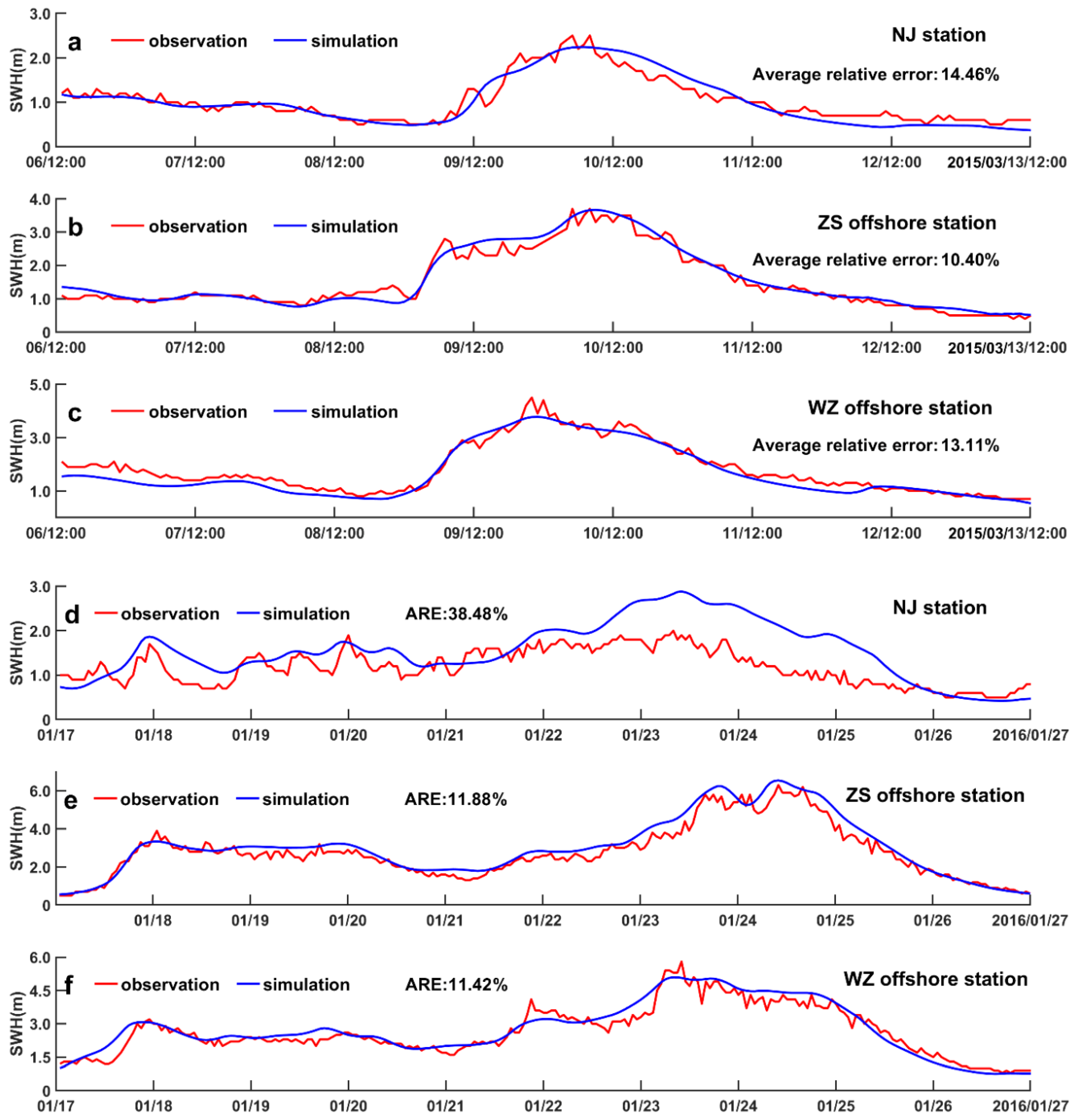
3.2. Model Validation

The waves induced by two typical cold front events (9 to 11 March 2015 and 22 to 25 January 2016) were simulated to verify the model. The east and south boundaries of the computational region were set as the open boundaries, and the discrete frequency range set to 0.04–1.00 Hz. To ensure stability and accuracy, the time step for the calculation was 20 min, and the wave parameters including the SWH and swell height were recorded hourly.

Figure 4 shows the difference between the simulated and observed SWHs at three stations during the two cold front events. Except for the NJ station, the model results are in accordance with the observations in magnitudes and phases. For the cold front event in 2015, the average relative errors for the NJ, ZS offshore, and WZ offshore stations are 14.46%, 10.40%, and 13.11%, respectively; for the cold front event in 2016, the corresponding average relative errors are 38.48%, 11.88%, and 11.42%, respectively. Possible sources of the errors are: (1) the spatiotemporal resolution of the CCMP wind field was insufficient; (2) the ETOPO-1 data was not accurate enough; (3) The grid used was not fine enough; (4) the limitations of the SWAN model itself and the errors introduced in the calculations. Overall, the SWAN model can be used to simulate the wave patterns induced by the cold fronts in the ECS.

The distribution of the simulated SWHs from 9 to 11 March 2015 is shown in Figure 5a–f. The cold front event lasted for about two days, resulting in a significant change in wave height in the study area. Specifically, the cold front first affected the Bohai Sea, which lasted for about a day, resulting in SWH rising more than 6 m. Then, the high wave area gradually moved eastward to the Yellow Sea and the ECS. The effect of the cold front eventually disappeared after two days. Figure 6a,c,e show the CCMP wind speed and direction during the cold front at the NJ station, ZS offshore station, and WZ offshore station, respectively. From 9 to 11 March 2015, the wind speeds at the three stations were at high levels, and the wind directions were mainly northwest. At the end of the cold front process, the wind speed and direction changed significantly, which coincided with the change of SWH in Figure 5.

On 22 January 2016, another strong cold front invaded the ECS. Figure 5g–l shows the SWH distribution during the event. The cold front induced large waves in the ECS and the SWH reached up to 8 m on 24 January 2016. Subsequently, the high wave height area gradually moved southeast, and the impact of the cold front gradually weakened and finally disappeared on 27 January 2016. In Figure 6b,d,f, it can be seen that the wind speeds of all three stations were at high levels, and the wind direction gradually shifted from north by west to north by east from 21 to 11 January 2016, which was different from the first cold front process. To sum up, in the two cold front events, although the trajectory of the high wave height region was southeast, they were not the same.

3.3. Sensitivity Numerical Experiments

3.3.1. Settings of Numerical Experiments

Previous studies have shown that atmospheric models can be used to simulate cold fronts [39,40]. For example, Guo et al. [41] studied the effect of atmospheric fronts on waves over the Louisiana continental shelf by comprehensively considering the influence of multiple atmospheric parameters including wind and pressure. In this section, an artificial wind field was constructed to represent the cold front winds. As the cold front is a long-term weather system usually lasting about three days, the wind speed and direction remain spatially constant in the artificial wind field [22]. As shown in Figure 7a, the cold front wind field is constructed as follows: (1) Beaufort Class 3 (3.4 m/s) is taken as the normal wind speed; (2) when the wind speed increases to Beaufort Class 6 (10.8 m/s) the study area enters the stage of cold front wind; (3) the wind speed of the cold front increases to the maximum value of the Beaufort Class 8 (20.7 m/s) and then decreases to 10.8 m/s. The cold front wind duration is set as 20 h. To make the wind speed variation more smooth and natural, the original linear function was replaced by a quadratic function, which keeps the slope consistent when the stage changes. The improved cold front wind field model adopted in this study is shown in Figure 7b.

Waves induced by cold front winds can be affected by many factors including the track, intensity, and duration, etc., of cold fronts. In this paper, we focus on the influence of cold front wind directions. Key research areas are shown in Figure 7d,e, namely, the adjacent sea areas of Zhejiang (119–126 E, 27–35 N). The Sa and Sb station groups were established to analyze the temporal and spatial distribution of waves in the key research areas.

For simplification of the model, Zhao and Jiang [23] set constant directions for different cold front tracks. However, there are considerable differences in wind directions for different cold fronts. According to the conclusions of Section 3.1, the designed cold front wind directions in the ECS are mainly between 75° N.W and 75° N.E, which was divided into eleven directions with intervals of 15°, as shown in Figure 7c. Hence, eleven numerical experiments were designed to study the influence of wind directions on waves induced by the cold fronts. The numbers of these eleven numerical experiments were named Exp1-1, Exp1-2 … Exp1-11 from east to west, according to the wind direction.

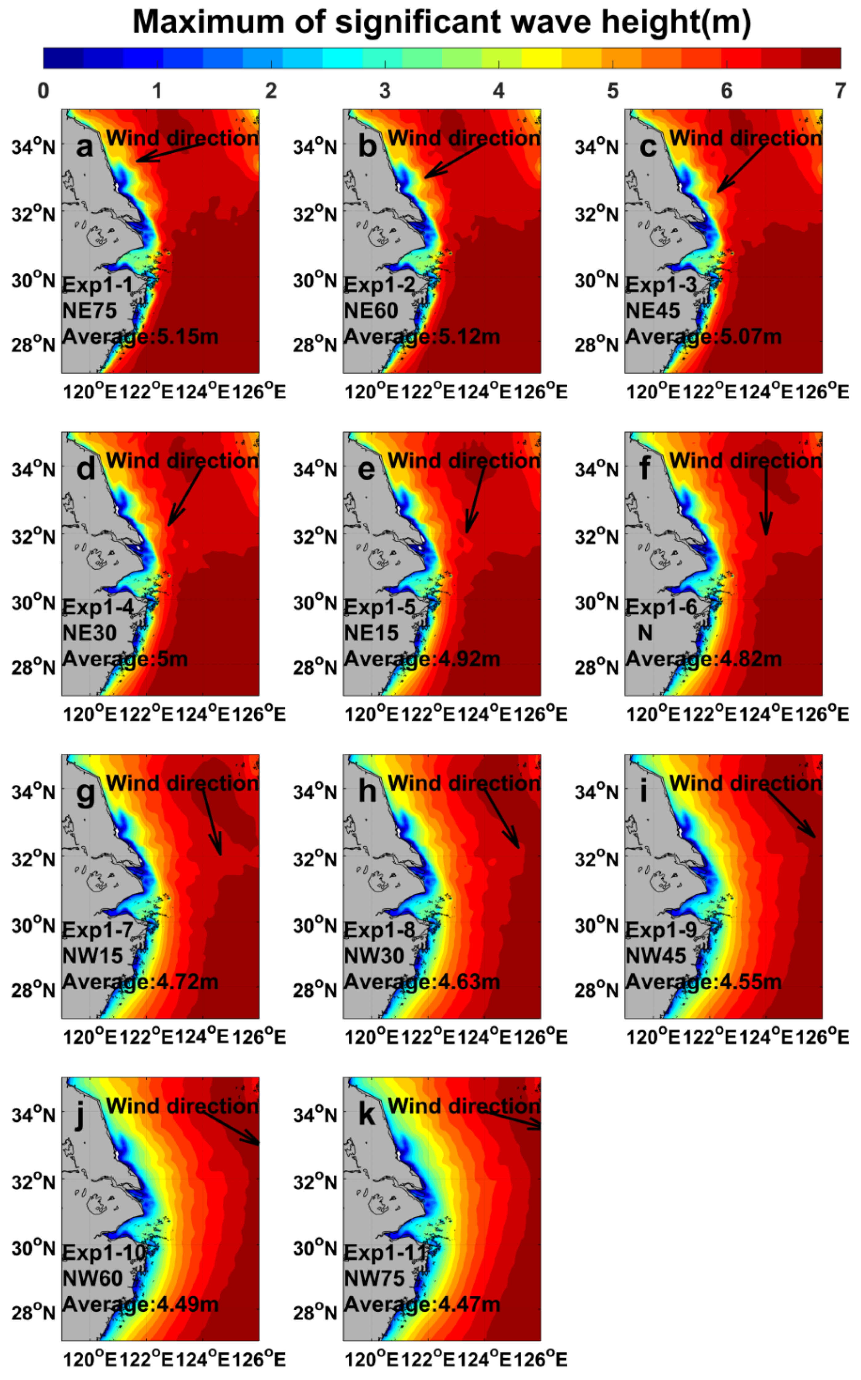
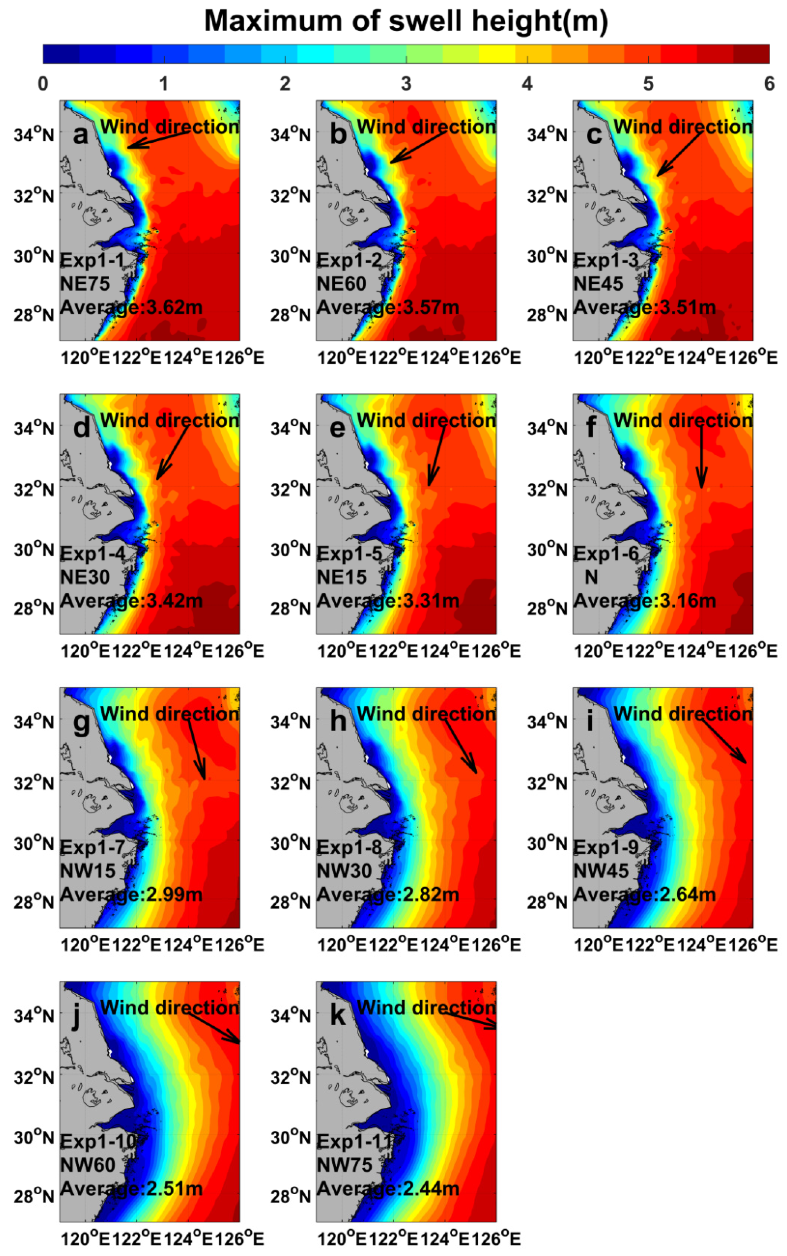
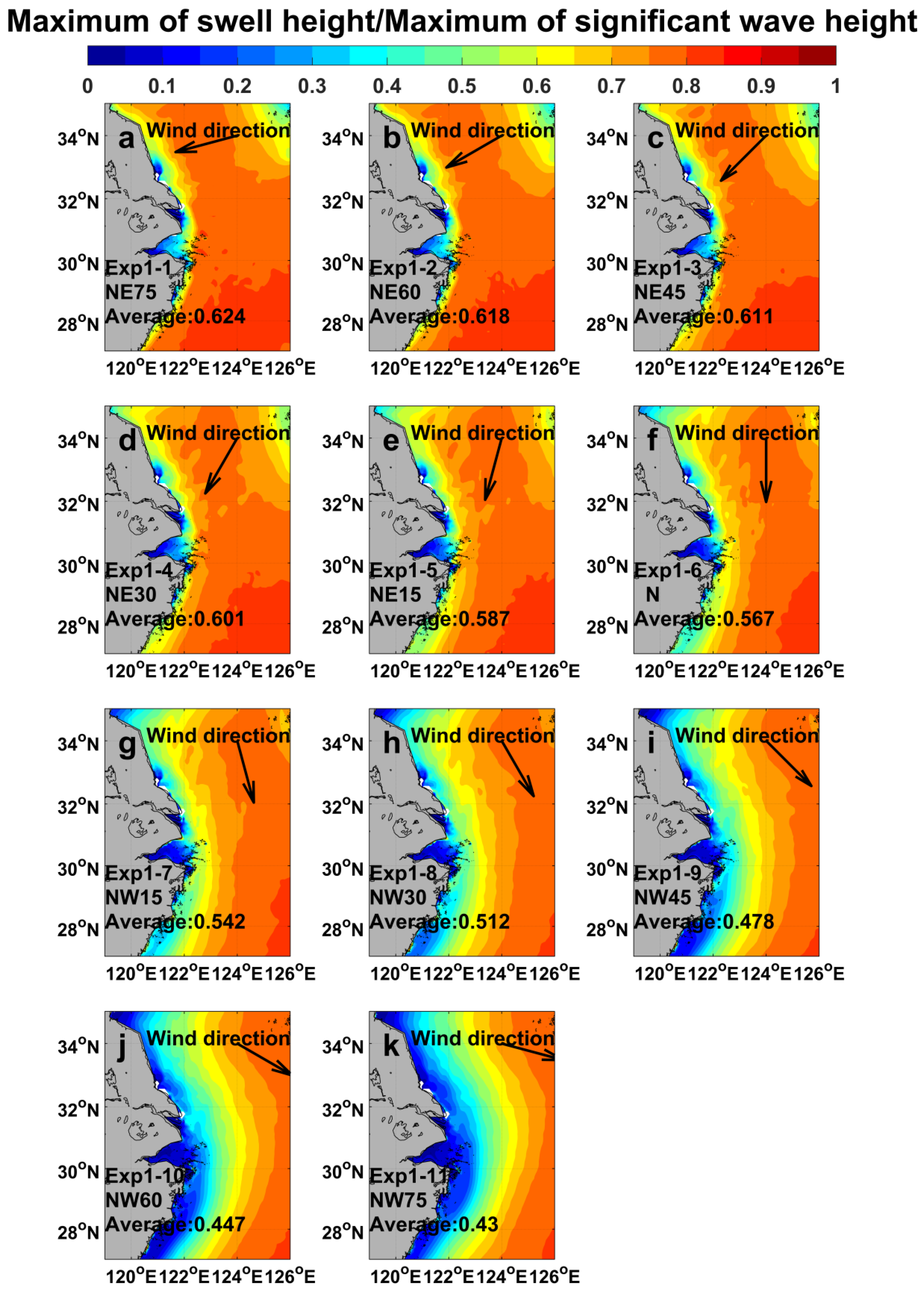
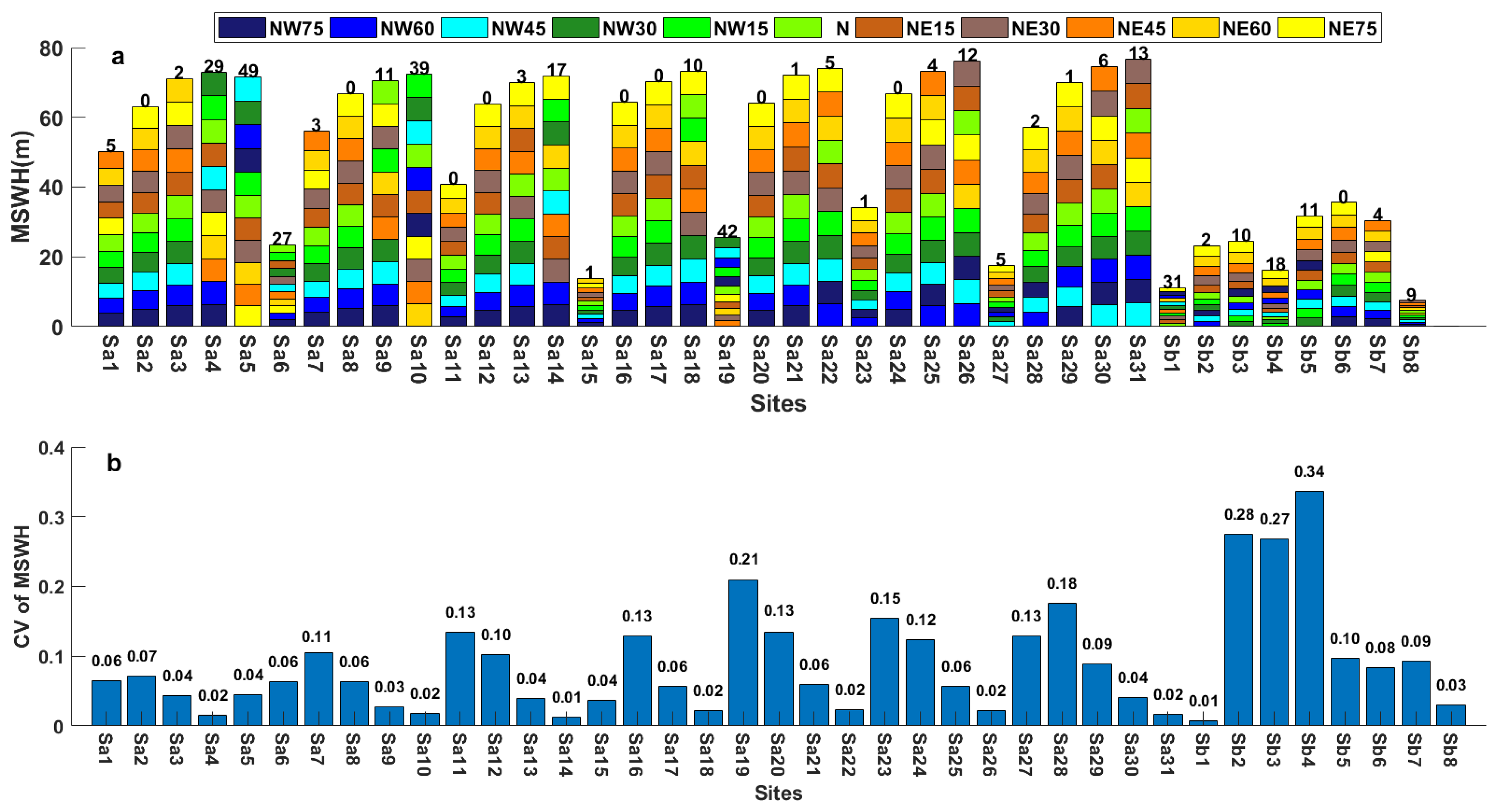
3.3.2. Spatial Distribution of MSWH Affected by Wind Direction

Figure 8 shows the spatial distribution of the maximum significant wave height (MSWH) during a cold front process in the study region in eleven experiments. It can be seen that MSWH increased from nearshore to deep sea. In addition, the gradient of MSWH near shore is greater than that in the open sea. The gradient of MSWH in the north of the study area was smaller than that in the south. For the northern stations, such as Sa1–5, MSWH first increases and then decreases with the increase of site longitude. However, for the southern stations such as Sa27–31, MSWH increases monotonically. Differences between the two regions probably can be explained by the presence of islands in the northeast. Water depth in the northern region first increases and then decreases with the increase of site longitude due to the presence of islands in the northeast, while the water depth in the southern region increases monotonically with the increase of site longitude.

3.3.3. Spatial Distribution of MSH Affected by Wind Direction

Figure 9 shows the spatial distribution of the maximum swell height (MSH) in eleven numerical experiments during the process of the cold front. It can be seen that the spatial distribution of MSH during a single cold front is the same as that of the mixed waves. To further understand whether the mixed waves dominate the swells in different locations offshore Zhejiang during the cold front, the MSH/MSWH was calculated for each station offshore Zhejiang (Figure 10). It can be seen that during a single cold front process, the nearshore waves are dominated by wind waves, while the offshore waves are dominated by swells.

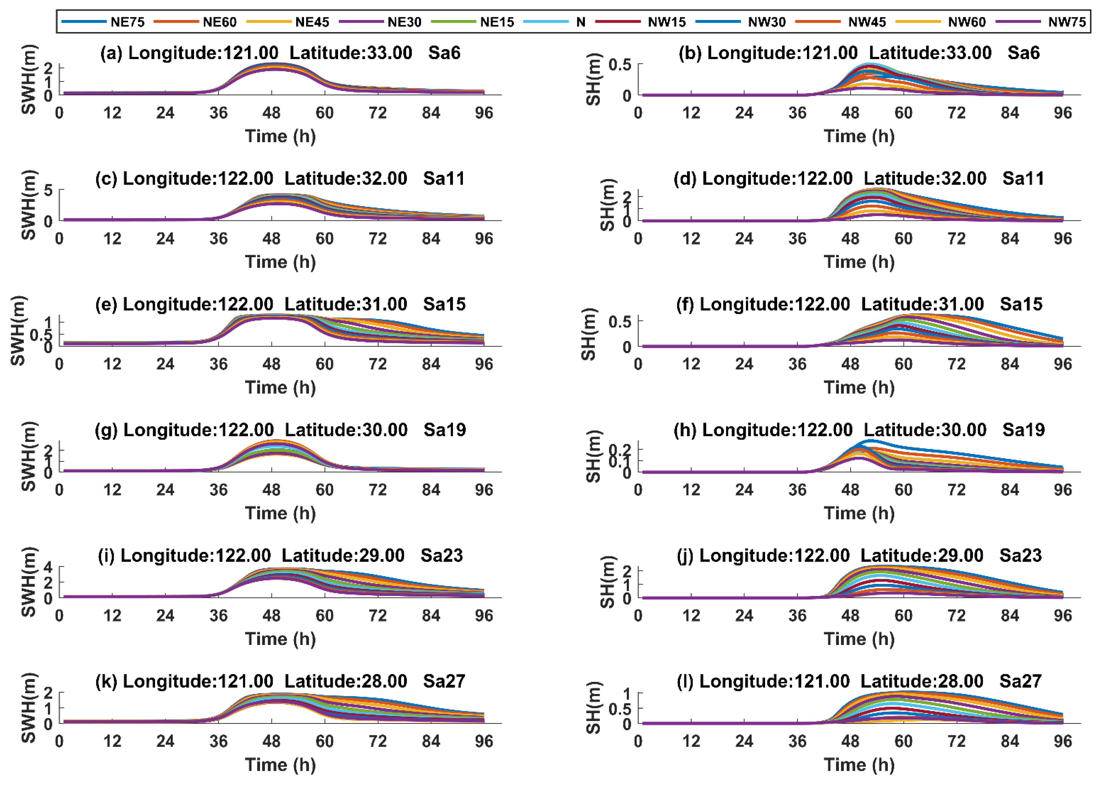
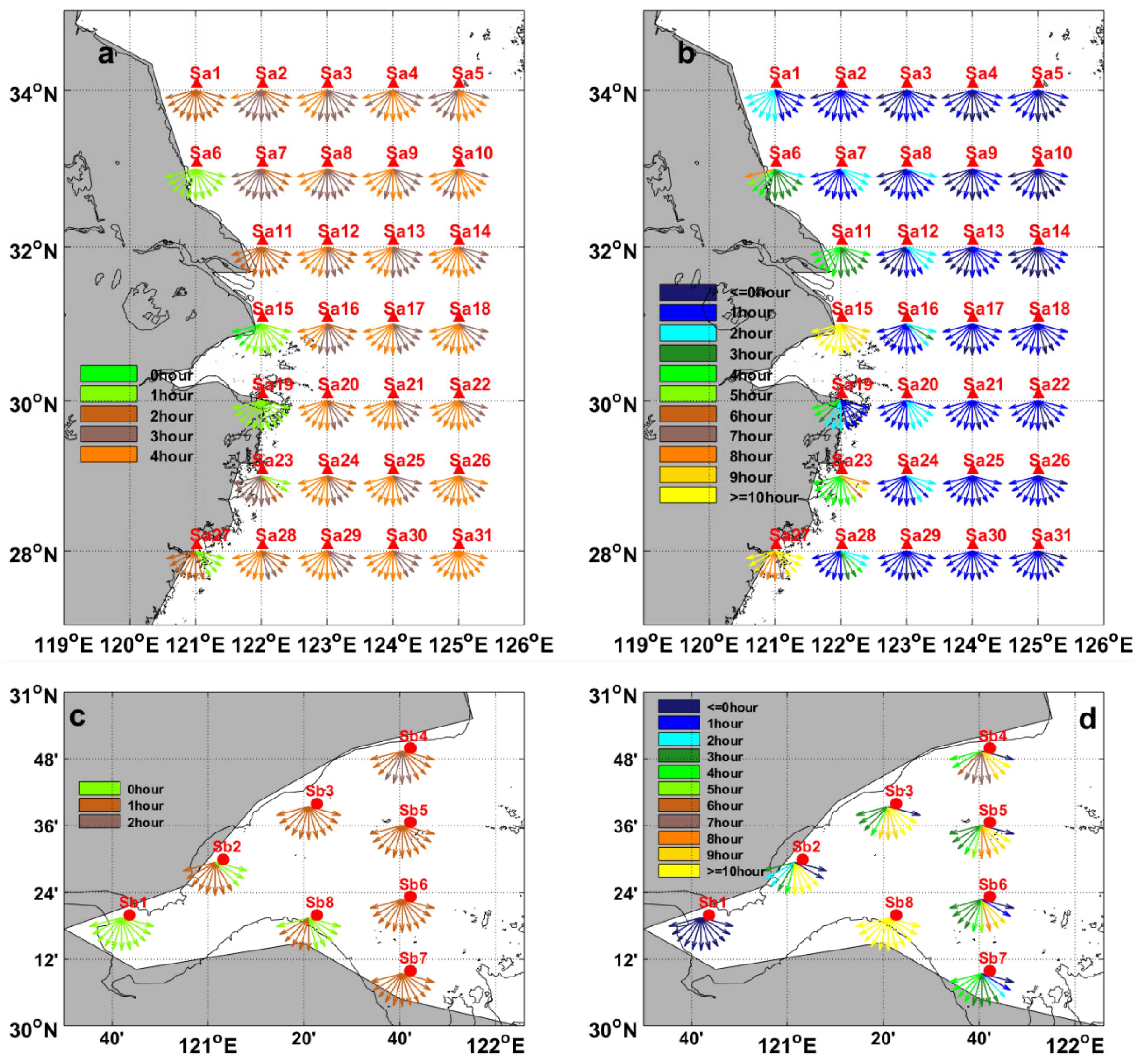
3.3.4. Temporal Variation of MSWH and MSH Affected by Wind Direction

Figure 11 shows the time difference between the occurrence of MSWH or MSH and the occurrence of maximum wind speed at each station in eleven numerical experiments. The direction of the arrow represents the wind direction of the cold front in each group of experiments, and the color of the arrow indicates the time difference. It can be seen that in all numerical experiments, the difference between the appearance time of MSWH and the appearance time of maximum wind speed (MWS) is within 4 h. For the same station, the time difference corresponding to the different directions of the cold front is different. For most stations, the northeast direction of the cold front corresponds to a greater time difference than the northwest direction.

For the nearshore stations, the time difference between the occurrence of MSWH and the occurrence of MWS was smaller than the offshore stations. For swells, the time difference between MSWH and MWS at stations farther offshore was within 3 h, and the time difference changed little under the influence of cold fronts in different wind directions. However, the time difference varied greatly at several nearshore stations, Sa6, 11, 15, 19, 23, and 27. The occurrence of MSH at these stations was later than at the other stations, and the occurrence time at the same station under the influence of cold fronts in different wind directions was also significantly different. The occurrence time of the cold front had no obvious correlation with the wind direction of the cold front. Similar results were obtained for Sb stations located in Hangzhou Bay (Figure 11c,d).

By further analyzing the exception sites found in the previous sections, the temporal variation of offshore swells in Zhejiang during the cold front process was studied. As can be seen in Figure 12, during the weakening of the cold front the SWH of these abnormal stations declined slowly compared with other stations, especially Sa15, 23, and 27. Taking Sa15 as an example, as shown in Figure 12e,f, when the wind direction is 75° north by east the temporal variation curve of SWH shows a flat cross-section. Due to the propagation characteristics of the swell, the peak value of SWH at the station appears later. When the wind direction was N.E. and the wind speed weakened, the swell contributed a larger proportion in the mixed waves, thus reducing the weakening speed of SWH. This phenomenon indicates that SWH may be at a high level for a long time in some areas, such as the exception area near Zhejiang, when a northeasterly cold front occurs. Due to the propagation of swells, the MSWH occurs slightly later than the maximum wind speed and becomes more pronounced in nearshore areas, increasing the duration of catastrophic waves.

4. Discussion

Statistical data obtained from numerical experiments are shown in

Table 2. Statistical Results of Numerical Experiments.

No.	Direction	Average MSWH (m)	Average MSH (m)	Average MSH/MSWH
Exp1-1	NE75	5.15	3.62	0.624
Exp1-2	NE60	5.12	3.57	0.618
Exp1-3	NE45	5.07	3.51	0.611
Exp1-4	NE30	5.00	3.42	0.601
Exp1-5	NE15	4.92	3.31	0.587
Exp1-6	N	4.82	3.16	0.567
Exp1-7	NW15	4.72	2.99	0.542
Exp1-8	NW30	4.63	2.82	0.512
Exp1-9	NW45	4.55	2.64	0.478
Exp1-10	NW60	4.49	2.51	0.447
Exp1-11	NW75	4.47	2.44	0.430

. The averaged MSWH of the ECS decreased when the wind direction shifted from 75° N.E to 75° N.W. As can be seen from Figure 8, the gradient of MSWH in the longitude direction decreased, probably because the calculated sea area is located on the east side of the continent. When the wind direction is deflected from west to east, the wind passes over the land, resulting in a shorter duration. Therefore, catastrophic waves are more likely to occur when an eastward cold front occurs offshore in the coastal area of Zhejiang.

According to the above analysis, when the wind direction changes from 75° N.E to 75° N.W, the mean MSWH of the calculated region decreases (Table 2). To determine whether the wind direction change pattern of MSWH at each station matches the overall pattern of ECS, the MSWH of each station is shown in Figure 13. MSWH occurring at each station under eleven wind direction conditions were arranged in the order from 75° north by west to 75° north by east, forming 39 permutations. The elements (MSWH) inside these permutations were not ordered from small to large; therefore, the reverse-ordered number of these permutations can be calculated to reflect the degree of confusion of this permutation. The inversion number of these permutations was calculated and recorded in Figure 14a. If the inversion number of a permutation is too large, it indicates that the station corresponding to this permutation deviates significantly from the overall pattern and can be recognized as an anomalous station. The stacked histogram in Figure 14a is a summary of Figure 13a,b; for any site, the larger MSWH is closer to the top of the histogram.

From Figure 14a, the inversion number at most stations is less than fifteen, in line with the general pattern of the east cold front being more dangerous than the west cold front. Several stations, Sa4, 5, 10, 6, 19, and Sb1, deviated significantly from the overall pattern. As can be seen in Figure 7e for Sa4, 5, 10, and 19, when the cold front occurred on the east side, the uplift was truncated by land because there were islands on the east side. The anomalies of Sb1 and Sa6 may be due to other geographical reasons, and need to be further analyzed. For these sites, a north cold front is more likely to cause catastrophic waves than a northeast one.

During the eleven cold fronts, the mean MSWH of stations farther from the coast did not change significantly with latitude, but increased slightly with longitude. The spatial variability of the mean MSWH in the nearshore area of each station was larger and lacking regularity.

The coefficient of variation (CV) can measure the dispersion of a set of data. The eleven MSWH records obtained by a site in eleven groups of experiments can be seen as a set of data. The CV of this set of data can reflect the sensitivity of the station to the wind direction of cold front. The CV of MSWH at each station during eleven cold fronts is calculated and shown in the form of a histogram in Figure 14b. It can be seen that the CV of Sb2, 3, and 4 stations, located on the north bank of Hangzhou Bay, is significantly higher than that of the other stations. This indicates that the sensitivity of the northern stations to cold front wind direction is higher than that of the southern stations. The CV values of Sa4, 10, 14, 18, 22, 26, and 31 stations are small and distributed in the area with large water depth. The CV of Sb1 and eight stations in Hangzhou Bay is also less than normal, which may be caused by the low water depth.

For swell, when the wind was directed from N.E75 to N.W75, the average value of the MSH in the whole domain decreased, which is consistent with that of MSWH. From Table 2, the average value of the ratio of the MSH and the MSWH decreased with the change in wind direction. When the wind was deflected, the value dropped from 62% to 43%, indicating that waves gradually changed from swell-dominated to wind-dominated. Therefore, when the eastern cold front occurs in Zhejiang, more attention should be paid to the occurrence of swell disasters.

5. Conclusions

Two typical cold front events in the coastal area of Zhejiang were simulated. The comparison between SWH simulation results and observations shows that the SWAN model forced by the CCMP wind field is feasible to simulate cold front-induced waves. Based on the CCMP wind field data, the days with north wind greater than 17.2 m/s in the past ten years, from 2004 to 2013, were counted. The results showed that the number of days affected by strong northerly winds in northeast China accounted for 16.86% of the total number of days. Among them, the ECS is mainly invaded by strong northerly winds from August to April. Strong northerly invasions accounted for 88.1% of the total number of days in the eight months. The monthly wind direction statistics show that except for August, the winds are mainly northeast, with a few winds in the northwest remaining between 75° W and 75° E. From September to December, the proportion of northeast wind increased by month, while from January to April, the proportion of the northeast wind decreased by month.

Based on the above analysis, we designed eleven groups of numerical experiments to study the influence of cold front wind direction on the spatial-temporal distribution characteristics of cold front-induced waves in Zhejiang offshore waters. As the cold front direction deflected from N.E 75° to N.W 75°, the mean MSWH, mean MSH, and mean MSH/MSWH all decreased. A few nearshore stations, such as Sa5 and Sa10, did not fit this pattern due to topography, water depth, etc. In addition, it was found that swells have a great influence on the increasing of duration of SWH exceeding the threshold. The practical significance of this study is the finding that when the offshore area of Zhejiang is affected by a northeast cold front, disastrous waves are more likely to occur than during a northwest cold front; thus, disaster prevention work should be done in advance. Coastal areas should pay attention to the occurrence of swell disasters.

In this work, the obvious deficiency is that there is a large deviation between the observed and simulated SWHs at NJ station in the simulation of the cold front in 2016. However, the simulation results of cold front-induced waves at NJ station in 2015 are acceptable. Therefore, in future work more cold front processes in the ECS need to be simulated in order to check the reliability of the model at NJ station; the observed SH can also be used to compare with the simulation results to make the results more reliable. A grid with improved accuracy could further improve the correctness of simulation results as well.

References

1. Wang, Z.; Ding, Y. Climate change of the cold wave frequency of China in the last 53 years and the possible reasons. J. Lake Sci. 2006, 30, 1068–1076. [Google Scholar] [CrossRef]
2. Rey, W.; Salles, P.; Mendoza, E.T.; Torres-Freyermuth, A.; Appendini, C.M. Assessment of coastal flooding and associated hydrodynamic processes on the south-eastern coast of Mexico, during Central American cold surge events. Nat. Hazards Earth Syst. Sci. 2018, 18, 1681–1701. [Google Scholar] [CrossRef] [Green Version]
3. Bevington, A.E.; Twilley, R.R.; Sasser, C.E.; Holm, G.O. Contribution of river floods, hurricanes, and cold fronts to elevation change in a deltaic floodplain, northern Gulf of Mexico, USA. Estuar. Coast. Shelf Sci. 2017, 191, 188–200. [Google Scholar] [CrossRef] [Green Version]
4. Huang, W.; Li, C. Contrasting Hydrodynamic Responses to Atmospheric Systems with Different Scales: Impact of Cold Fronts vs. That of a Hurricane. J. Mar. Sci. Eng. 2020, 8, 979. [Google Scholar] [CrossRef]
5. Appendini, C.M.; Hernández-Lasheras, J.; Meza-Padilla, R.; Kurczyn, J.A. Effect of climate change on wind waves generated by anticyclonic cold front intrusions in the Gulf of Mexico. Clim. Dyn. 2018, 51, 3747–3763. [Google Scholar] [CrossRef]
6. Chen, T.; Yen, M.; Huang, W. An East Asian Cold Surge: Case Study. Mon. Weather Rev. 2001, 130, 2271–2290. [Google Scholar] [CrossRef]
7. Ding, Y.H. Build-Up, Air Mass Transformation and Propagation of Siberian High and Its Relations to Cold Surge in East Asia. Meteorol. Atmos. Phys. 1990, 44, 281–292. [Google Scholar] [CrossRef]
8. Liu, W.; Huang, S.-Y.; Li, D.; Wang, C.-Y.; Zhou, X.; Chen, S.-S. Spatiotemporal computing of cold wave characteristic in recent 52 years: A case study in Guangdong Province, South China. Nat. Hazards 2015, 79, 1257–1274. [Google Scholar] [CrossRef] [Green Version]
9. Tomczyk, A.M.; Półrolniczak, M.; Kolendowicz, L. Cold Waves in Poznań (Poland) and Thermal Conditions in the City during Selected Cold Waves. Atmosphere 2018, 9, 208. [Google Scholar] [CrossRef] [Green Version]
10. Zhao, Q.; Ding, Y. Study of physical processes affecting the transformation of cold air over land after outbreak of cold waves in east Asia. J. Meteorol. Res. 1992, 6, 198–212. [Google Scholar]
11. Liu, X.; Zhu, X.; Pan, Y.; Zhao, A.; Li, Y. Spatiotemporal changes of cold surges in Inner Mongolia between 1960 and 2012. J. Geogr. Sci. 2015, 25, 259–273. [Google Scholar] [CrossRef]
12. Hsueh, Y.; Romea, R.D.; DeWitt, P.W. Wintertime Winds and Coastal Sea-Level Fluctuations in the Northeast China Sea. Part II: Numerical Model. J. Phys. Oceanogr. 1986, 16, 241–261. [Google Scholar] [CrossRef] [Green Version]
13. Ortiz-Royero, J.C.; Otero, L.J.; Restrepo, J.C.; Ruiz, J.; Cadena, M. Cold fronts in the Colombian Caribbean Sea and their relationship to extreme wave events. Nat. Hazards Earth Syst. Sci. 2013, 13, 2797–2804. [Google Scholar] [CrossRef] [Green Version]
14. Payandeh, A.; Justic, D.; Mariotti, G.; Huang, H.; Sorourian, S. Subtidal Water Level and Current Variability in a Bar—Built Estuary During Cold Front Season: Barataria Bay, Gulf of Mexico. J. Geophys. Res. Oceans 2019, 124, 7226–7246. [Google Scholar] [CrossRef]
15. Li, C.; Huang, W.; Milan, B. Atmospheric Cold Front–Induced Exchange Flows through a Microtidal Multi-Inlet Bay: Analysis Using Multiple Horizontal ADCPs and FVCOM Simulations. J. Atmos. Ocean. Technol. 2019, 36, 443–472. [Google Scholar] [CrossRef]
16. Weeks, E.; Robinson, M.E.; Li, C. Quantifying cold front induced water transport of a bay with in situ observations using manned and unmanned boats. Acta Oceanol. Sin. 2018, 37, 1–7. [Google Scholar] [CrossRef]
17. Huang, W.; Li, C. Cold Front Driven Flows Through Multiple Inlets of Lake Pontchartrain Estuary. J. Geophys. Res. Oceans 2017, 122, 8627–8645. [Google Scholar] [CrossRef] [Green Version]
18. Li, Y.; Li, C.; Li, X. Remote Sensing Studies of Suspended Sediment Concentration Variations in a Coastal Bay During the Passages of Atmospheric Cold Fronts. IEEE J. Sel. Top. Appl. Earth Obs. Remote Sens. 2017, 10, 2608–2622. [Google Scholar] [CrossRef]
19. Cao, Y.; Li, C.; Dong, C. Atmospheric Cold Front-Generated Waves in the Coastal Louisiana. J. Mar. Sci. Eng. 2020, 8, 900. [Google Scholar] [CrossRef]
20. Mo, D.; Hou, Y.; Liu, Y.; Li, J. Study on the growth of wind wave frequency spectra generated by cold waves in the northern East China Sea. J. Oceanol. Limnol. 2018, 36, 1509–1526. [Google Scholar] [CrossRef]
21. Li, X.; Dong, S. A preliminary study on the intensity of cold wave storm surges of Laizhou Bay. J. Ocean Univ. China 2016, 15, 987–995. [Google Scholar] [CrossRef]
22. Mo, D.; Hou, Y.; Li, J.; Liu, Y. Study on the storm surges induced by cold waves in the Northern East China Sea. J. Mar. Syst. 2016, 160, 26–39. [Google Scholar] [CrossRef]
23. Zhao, P.; Jiang, W. A numerical study of storm surges caused by cold-air outbreaks in the Bohai Sea. Nat. Hazards 2011, 59, 1–15. [Google Scholar] [CrossRef]
24. Zheng, G.; Zhao, H.; Xu, F.; Zhang, S.H. Numerical simulation of wind waves in Bohai Sea induced by “98.04” cold wave. Port Waterw. Eng. 2010, 2, 36–39. [Google Scholar]
25. Zhou, C.; Xu, F. Research on the numerical simulation of wind wave field affected by a cold wave in Jiangsu coast. Ocean Eng. 2017, 35, 123–130. [Google Scholar] [CrossRef]
26. Borkowski, P. Numerical Modeling of Wave Disturbances in the Process of Ship Movement Control. Algorithms 2018, 11, 130. [Google Scholar] [CrossRef] [Green Version]
27. Atlas, R.; Ardizzone, J.; Hoffman, R.N. Application of satellite surface wind data to ocean wind analysis. Proc. SPIE Int. Soc. Opt. Eng. 2008, 7087, 70870. [Google Scholar] [CrossRef]
28. Zhang, H.; Gu, J.; Wang, H. Simulating wind wave field near the Pearl River Estuary with SWAN nested in WAVEWATCH. J. Trop. Oceanogr. 2013, 32, 8–17. [Google Scholar] [CrossRef]
29. Ying, W.; Zheng, Q.; Zhu, C.; Zhu, Y.; Che, Z.; Chu, D.; Zhang, J. Numerical simulation of “CHAN-HOM” typhoon waves using SWAN model. Mar. Sci. 2017, 41, 108–117. [Google Scholar] [CrossRef]
30. Holthuijsen, L.H.; Booij, N.; Ris, R.C. A Spectral Wave Model for the Coastal Zone. In Ocean Wave Measurement and Analysis; ASCE: Reston, VA, USA, 1994; pp. 844–845. [Google Scholar]
31. Akpınar, A.; Bingölbali, B.; Van Vledder, G. Wind and wave characteristics in the Black Sea based on the SWAN wave model forced with the CFSR winds. Ocean Eng. 2016, 126, 276–298. [Google Scholar] [CrossRef]
32. Mao, M.; van der Westhuysen, A.J.; Xia, M.; Schwab, D.J.; Chawla, A. Modeling wind waves from deep to shallow waters in Lake Michigan using unstructured SWAN. J. Geophys. Res. Oceans 2016, 121, 3836–3865. [Google Scholar] [CrossRef]
33. Ris, R.C.; Holthuijsen, L.H.; Booij, N. A third-generation wave model for coastal regions: 2. Verification. J. Geophys. Res. Space Phys. 1999, 104, 7667–7681. [Google Scholar] [CrossRef]
34. Booij, N.; Ris, R.C.; Holthuijsen, L.H. A third-generation wave model for coastal regions: 1. Model description and validation. J. Geophys. Res. Oceans 1999, 104, 7649–7666. [Google Scholar] [CrossRef] [Green Version]
35. Zijlema, M.; van der Westhuysen, A.J. On convergence behaviour and numerical accuracy in stationary SWAN simulations of nearshore wind wave spectra. Coast. Eng. 2005, 52, 237–256. [Google Scholar] [CrossRef]
36. Chu, D.; Zhang, J.; Wu, Y.; Jiao, X.; Qian, S. Sensitivities of modelling storm surge to bottom friction, wind drag coefficient, and meteorological product in the East China Sea. Estuar. Coast. Shelf Sci. 2019, 231, 106460. [Google Scholar] [CrossRef]
37. Ding, Y.H.; Krishnamurti, T.N. Heat budget of the Siberian high and the winter monsoon. Mon. Weather Rev. 1987, 115, 2428–2449. [Google Scholar] [CrossRef] [Green Version]
38. Monmonier, M. Defining the Wind: The Beaufort Scale, and How a 19th Century Admiral Turned Science into Poetry. Prof. Geogr. 2005, 57, 474–475. [Google Scholar] [CrossRef]
39. Zhang, X.H. The Statistical Characteristics and Physical Mechanics of Strong Winds in Bohai Sea; College of Oceanic and Atmospheric Sciences, Ocean University of China: Qingdao, China, 2003. [Google Scholar] [CrossRef]
40. Park, T.-W.; Ho, C.-H.; Deng, Y. A synoptic and dynamical characterization of wave-train and blocking cold surge over East Asia. Clim. Dyn. 2013, 43, 753–770. [Google Scholar] [CrossRef]
41. Guo, B.; Subrahmanyam, M.V.; Li, C. Waves on Louisiana Continental Shelf Influenced by Atmospheric Fronts. Sci. Rep. 2020, 10, 1–9. [Google Scholar] [CrossRef]
Figure 1. (a) Model domain and bathymetry; (b) Computational grid of the model; (c) Location of Nanji station, Wenzhou offshore station, and Zhoushan offshore station. The range of (c) is marked with a red rectangle in (a).
Jmse 09 01452 g001
Figure 2. The number of days affected by strong northward winds (over 17.2 m/s) in the ECS in each month during 2004–2013.
Jmse 09 01452 g002
Figure 3. Wind rose map in the ECS in (a) January, (b) February, (c) March, (d) April, (e) August, (f) September, (g) October, (h) November, (i) December.
Jmse 09 01452 g003
Figure 4. Comparison between the observed and simulated SWHs at (a) NJ station from 6 March 2015, to 13 March 2015, (b) ZS offshore station from 6 March 2015, to 13 March 2015, (c) WZ offshore station from 6 March 2015, to 13 March 2015, (d) NJ station from 17 January 2016, to 27 January 2016, (e) ZS offshore station from 17 January 2016, to 27 January 2016, and (f) WZ offshore station from 17 January 2016, to 27 January 2016.
Jmse 09 01452 g004
Figure 5. (af) The distribution of simulated SWHs in the ECS from 9 March 2015, to 11 March 2015. (gl) Same as (af), from 22 January 2016, to 25 January 2016.
Jmse 09 01452 g005
Figure 6. CCMP wind speed and direction at (a) NJ station from 8 to 12 March 2015, (b) NJ station from 21 to 25 January 2016, (c) ZS offshore station from 8 to 12 March 2015, (d) ZS offshore station from 21 to 25 January 2016, (e) WZ offshore station from 8 to 12 March 2015, and (f) WZ offshore station from 21 to 25 January 2016.
Jmse 09 01452 g006
Figure 7. (a) Artificial wind field in previous studies; (b) Improved wind field used in the present study; (c) 11 cold-front wind directions: NW75 (75° north by west), NW60 (60° north by west), NW45 (45° north by west), NW30 (30° north by west), NW15 (15° north by west), N (north), NE15 (15° north by east), NE30 (30° north by east), NE45 (45° north by east), NE60 (60° north by east), NE75 (75° north by east); (d) Station group Sb, Hangzhou Bay; (e) Station group Sa, offshore Zhejiang.
Jmse 09 01452 g007
Figure 8. The distribution of the MSWH in the study region in (a) numerical experiment Exp 1-1, (b) numerical experiment Exp 1-2, (c) numerical experiment Exp 1-3, (d) numerical experiment Exp 1-4, (e) numerical experiment Exp 1-5, (f) numerical experiment Exp 1-6, (g) numerical experiment Exp 1-7, (h) numerical experiment Exp 1-8, (i) numerical experiment Exp 1-9, (j) numerical experiment Exp 1-10, (k) numerical experiment Exp 1-11. MSWH increases from nearshore to deep sea. Mean MSWH decreases as the wind direction changes from 75° N.E to 75° N.W.
Jmse 09 01452 g008
Figure 9. The distribution of MSH in the study region in (a) numerical experiment Exp 1-1, (b) numerical experiment Exp 1-2, (c) numerical experiment Exp 1-3, (d) numerical experiment Exp 1-4, (e) numerical experiment Exp 1-5, (f) numerical experiment Exp 1-6, (g) numerical experiment Exp 1-7, (h) numerical experiment Exp 1-8, (i) numerical experiment Exp 1-9, (j) numerical experiment Exp 1-10, (k) numerical experiment Exp 1-11. Spatial distribution of MSH is the same as that of the mixed waves. Mean MSH decreases as the wind direction changes from 75° N.E to 75° N.W.
Jmse 09 01452 g009
Figure 10. The ratio of the MSH and MSWH (MSH/MSWH) in the study region in (a) numerical experiment Exp 1-1, (b) numerical experiment Exp 1-2, (c) numerical experiment Exp 1-3, (d) numerical experiment Exp 1-4, (e) numerical experiment Exp 1-5, (f) numerical experiment Exp 1-6, (g) numerical experiment Exp 1-7, (h) numerical experiment Exp 1-8, (i) numerical experiment Exp 1-9, (j) numerical experiment Exp 1-10, (k) numerical experiment Exp 1-11. The nearshore waves are dominated by wind waves, while the offshore waves are dominated by swells. The mean ratio of the MSH and MSWH decreases as the wind direction changes from 75° N.E to 75° N.W.
Jmse 09 01452 g010
Figure 11. (a) The time difference between the occurrence of MSWH and the occurrence of maximum wind speed (MWS) at Sa stations in eleven numerical experiments; (b) same, for the time difference between the occurrence of MSH and the occurrence of MWS; (c) same, for the Sb stations; (d) Same, for the Sb stations.
Jmse 09 01452 g011
Figure 12. Time series of SWH and swell height at (a,b) exception station (The difference of appearance time of MSH and the maximum wind speed was unacceptable) Sa6, (c,d) exception station Sa11, (e,f) exception station Sa15, (g,h) exception station Sa19, (i,j) exception station Sa23, (k,l) exception station Sa27.
Jmse 09 01452 g012
Figure 13. (a) The MSWH of Sa stations in offshore Zhejiang under the influence of cold fronts with different wind directions; (b) same; for Sb stations in Hangzhou Bay. The MSWH of each station in each experiment is arranged in ascending order (the larger MSWH is closer to the top of the respective histogram).
Jmse 09 01452 g013
Figure 14. (a) MSWH under different wind directions of 39 stations (the larger respective MSWH is at the top of each histogram). MSWH occurring at each station under eleven wind conditions, arranged in the order from 75° N.W to 75° N.E. The inversion number of these permutations was marked at the top of the stacked histogram. (b) The coefficients of variation (CV = SD/mean) were obtained by calculating the MSWH that occurred during the eleven cold fronts at each station.
Jmse 09 01452 g014