
CFD Investigation on Hydrodynamic Resistance of a Novel Subsea Shuttle Tanker


Abstract
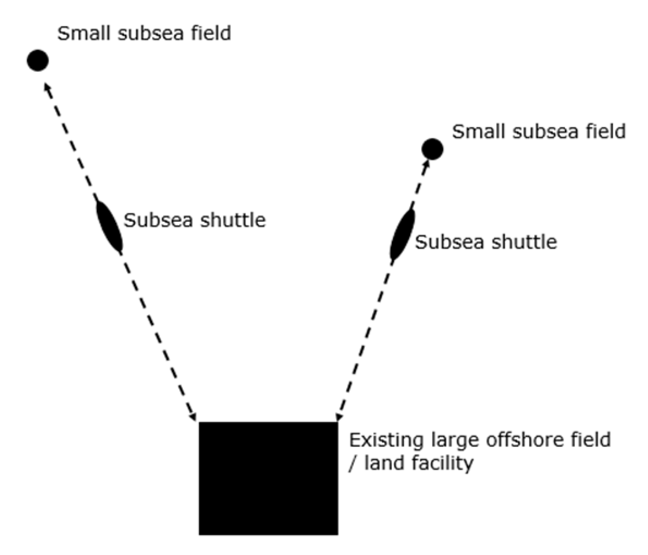
:1. Introduction
- It can carry hydrocarbons from a subsea well to a riser base with risers connected to a floating production unit (FPU) or land-based facility for processing.
- It can make use of pressure vessels mounted onboard to carry chemical fluids typically injected into subsea wells, such as methanol and glycol (MEG).
- It can transport electricity to subsea equipment. This can be achieved by storing the electrical power using onboard battery banks and transferring this to the subsea equipment while docked.
- It can also be configured to carry tools, structures, and modules required for subsea construction and intervention.
- The SST can avoid accidents induced by human factors.
- Submarine accidents are catastrophic since rescue and evacuation can be extremely difficult underwater. The cost of unexpected accidents will be significantly reduced for the SST as it is unmanned.
- The SST’s cargo capacity can be maximized as it does not require human support systems such as ventilation systems, freshwater tanks, control rooms, living quarters, or kitchens. This also means lower energy consumptions.
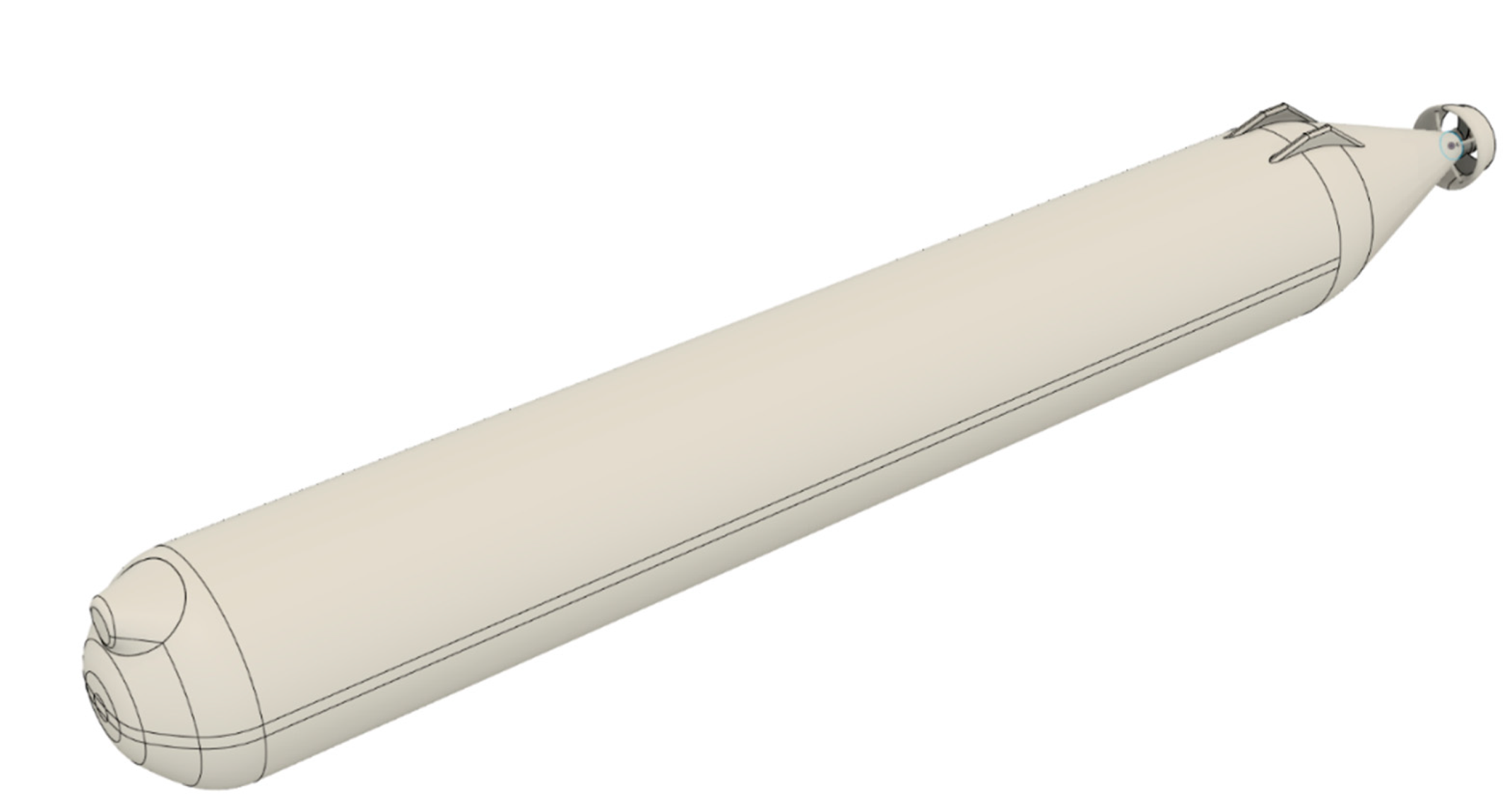
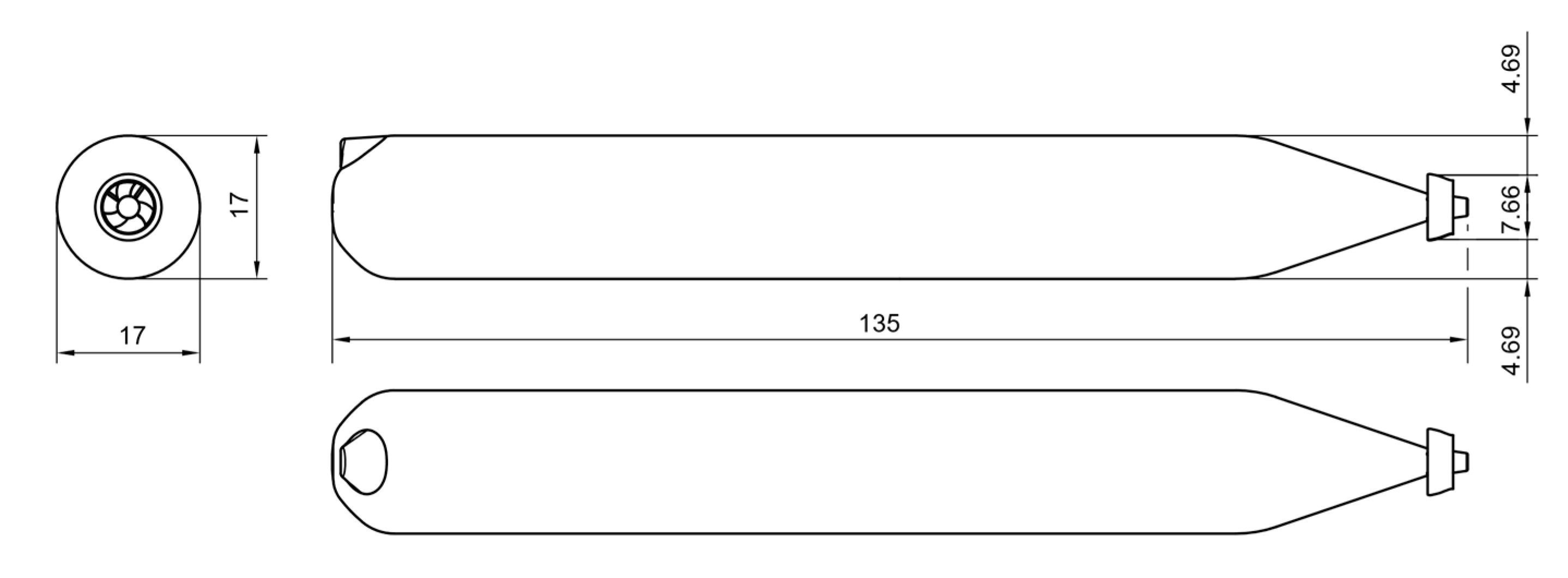
2. Main Design Parameters
3. Numerical Model
3.1. Numerical Method
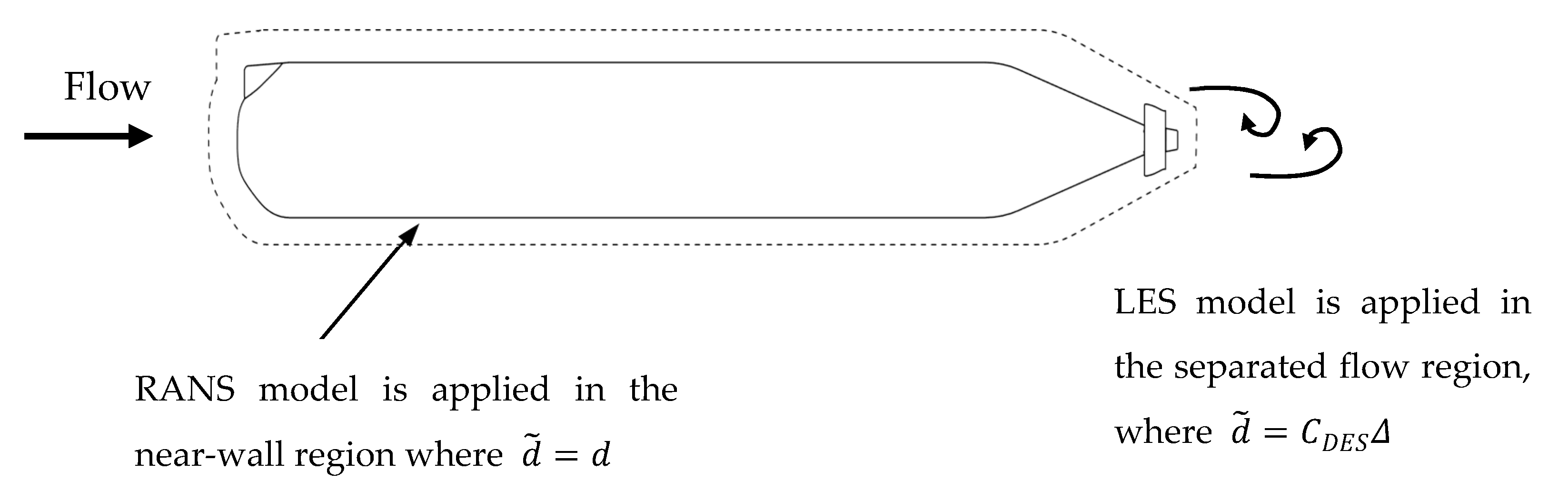
3.2. Turbulence Model
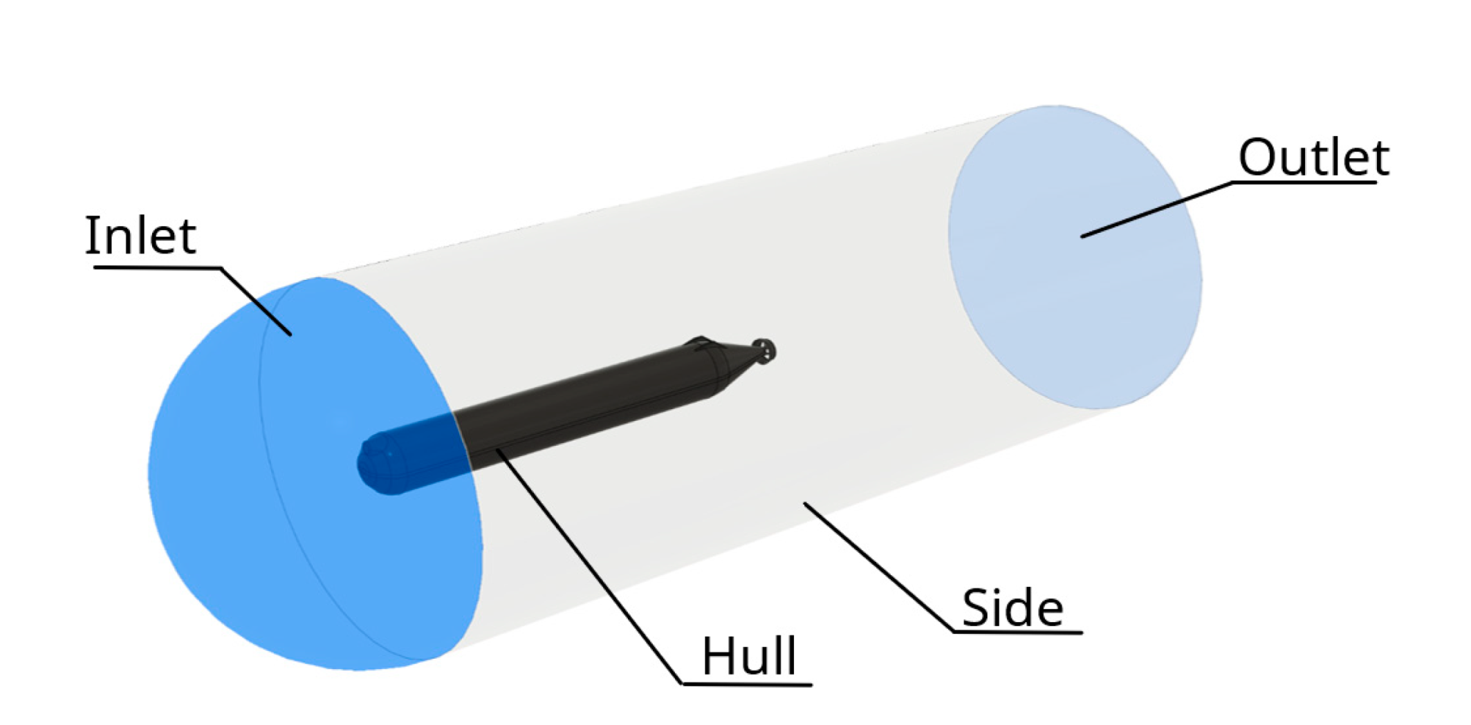
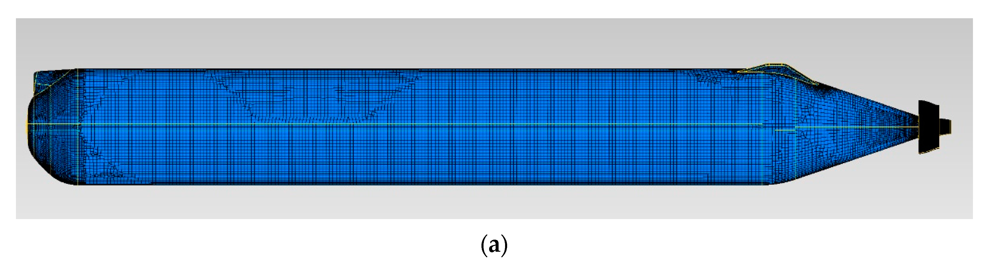
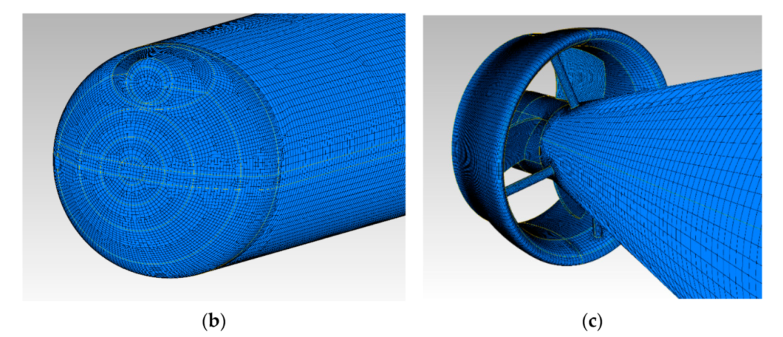
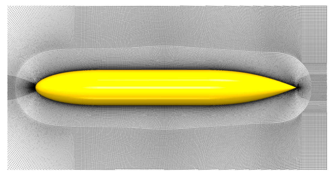
3.3. Computational Domain and Grid
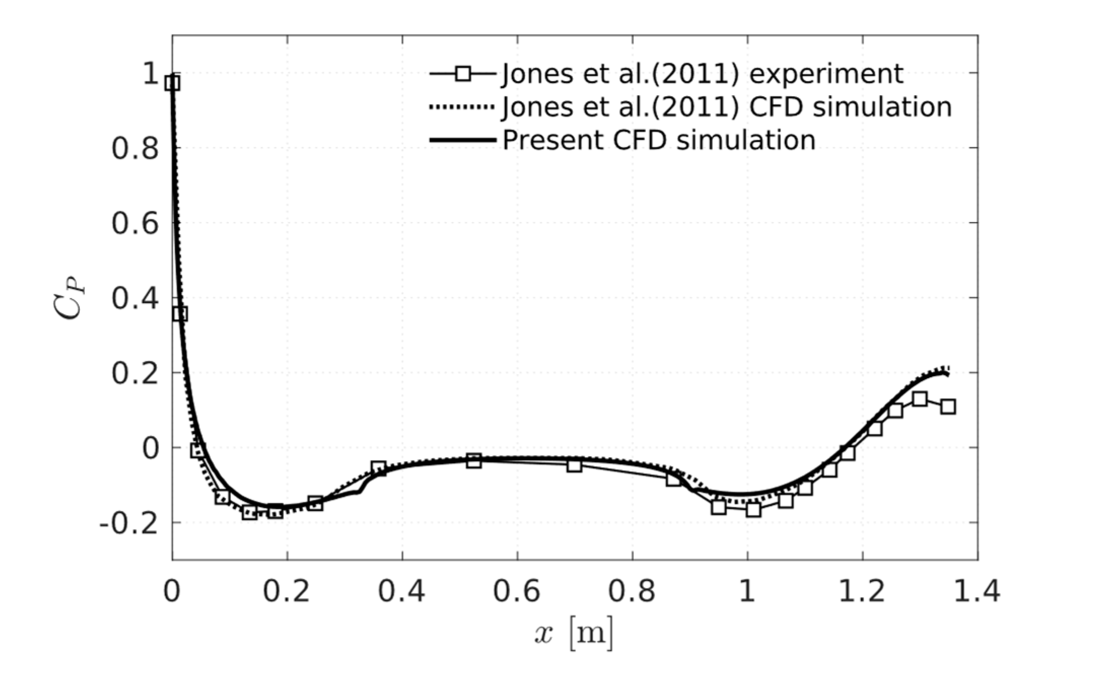
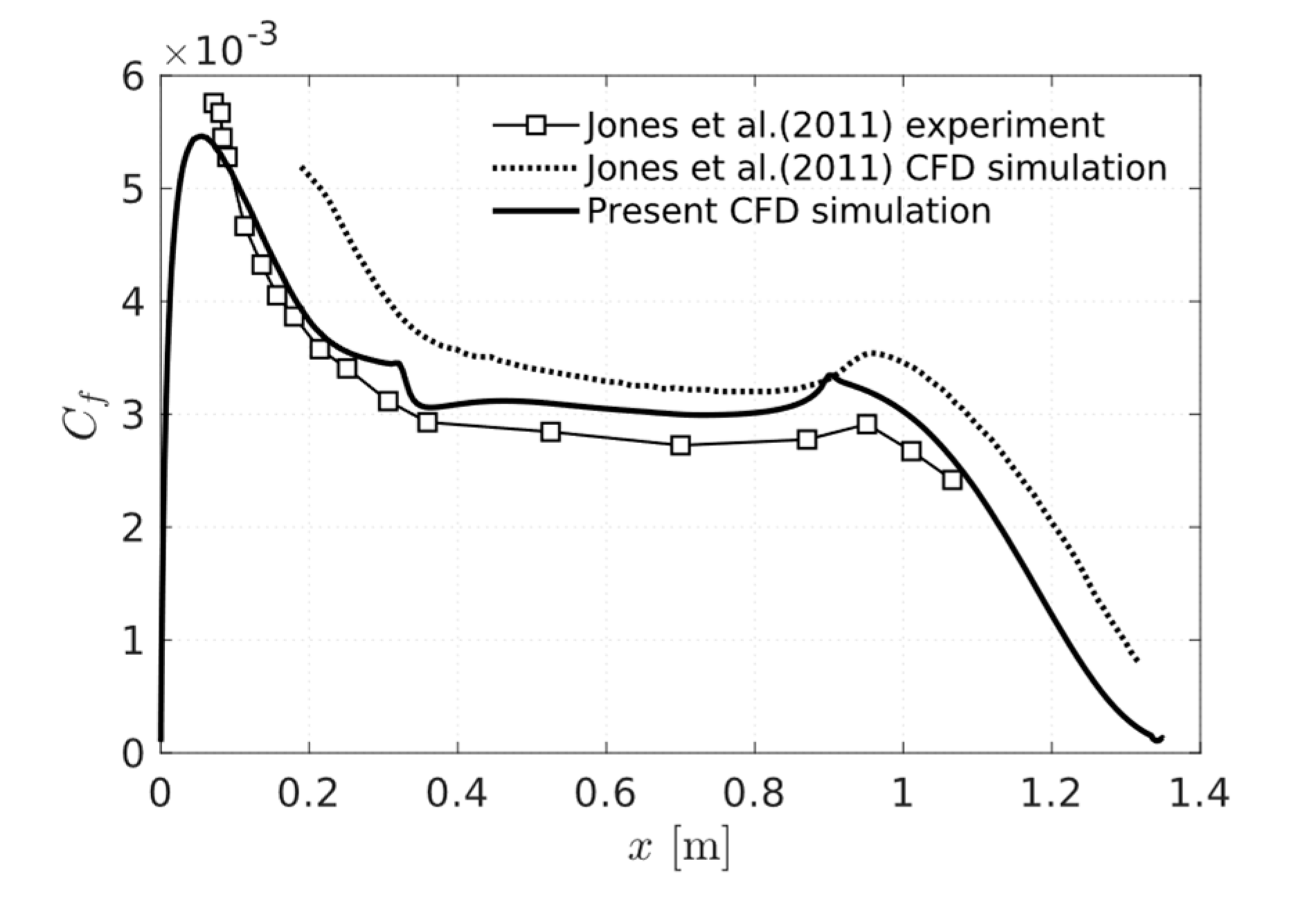
3.4. Verification and Validation
- Jones et al. (2011) experiment—Experimental results of Joubert’s hull geometry from Jones et al. [17]
- Jones et al. (2011) CFD simulation—CFD simulations results of Joubert’s hull geometry from Jones et al. [17]
- Present CFD simulation—CFD simulations results of Joubert’s hull geometry using the hybrid RANS/LES model which is utilized in this paper’s SST hull resistance study
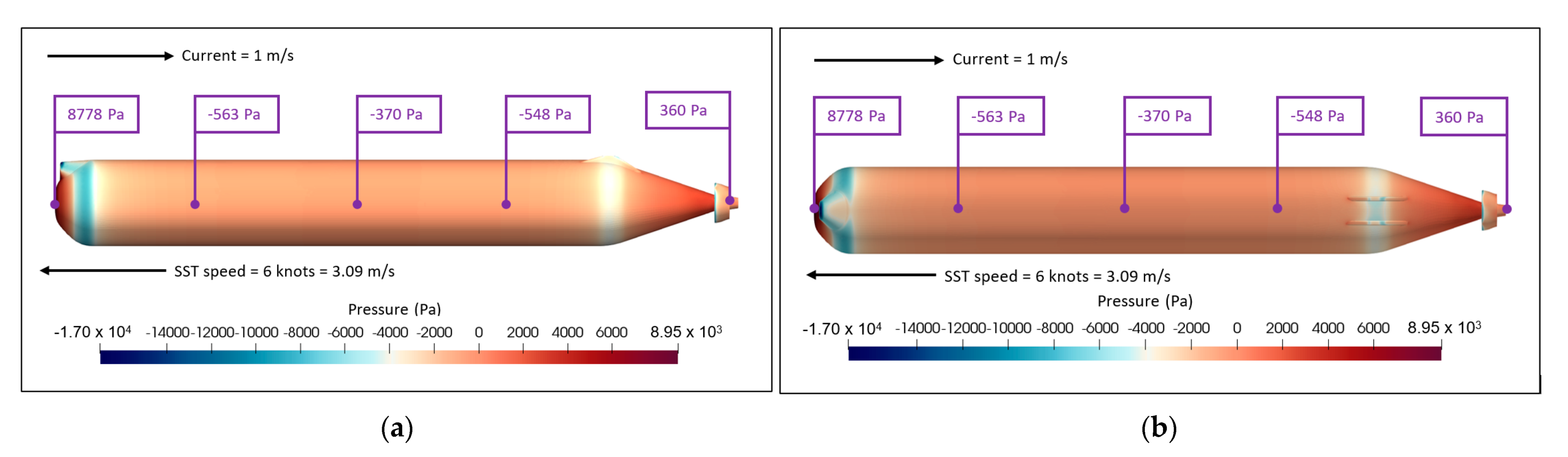
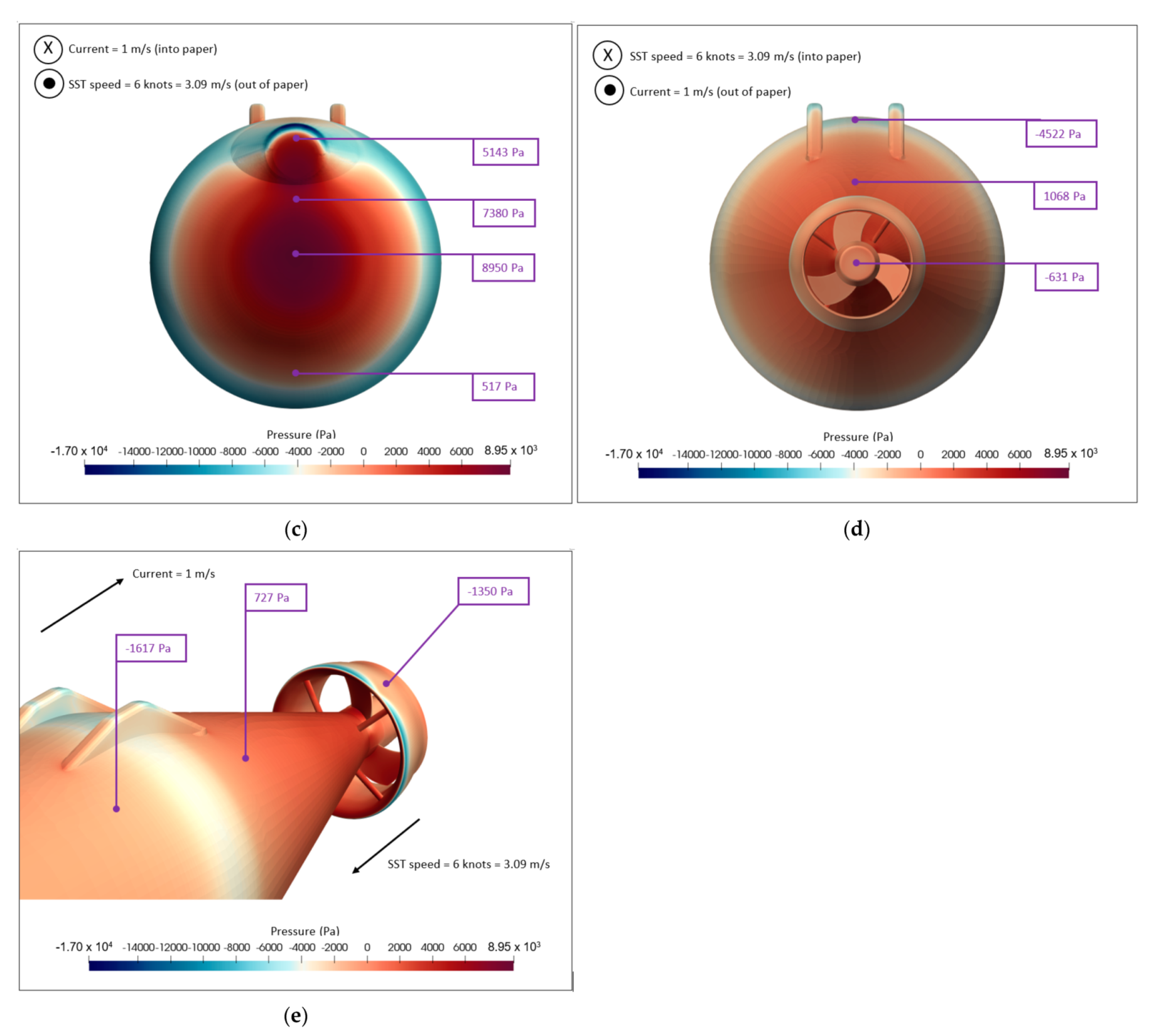
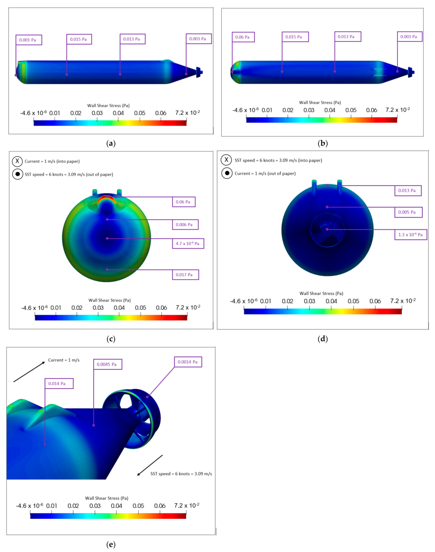
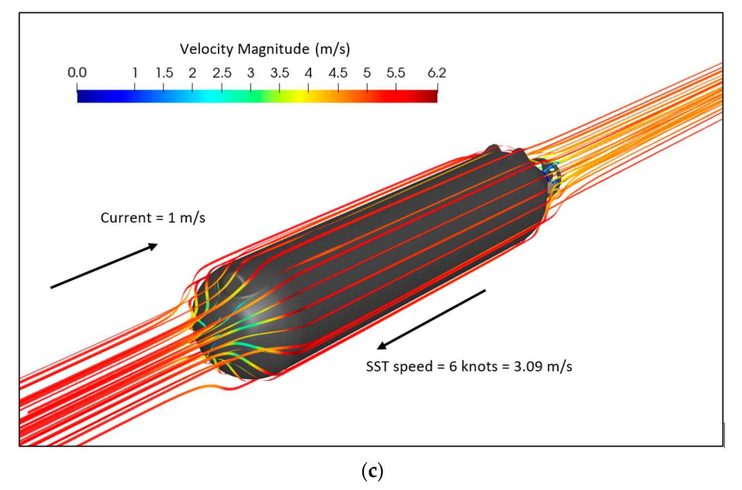
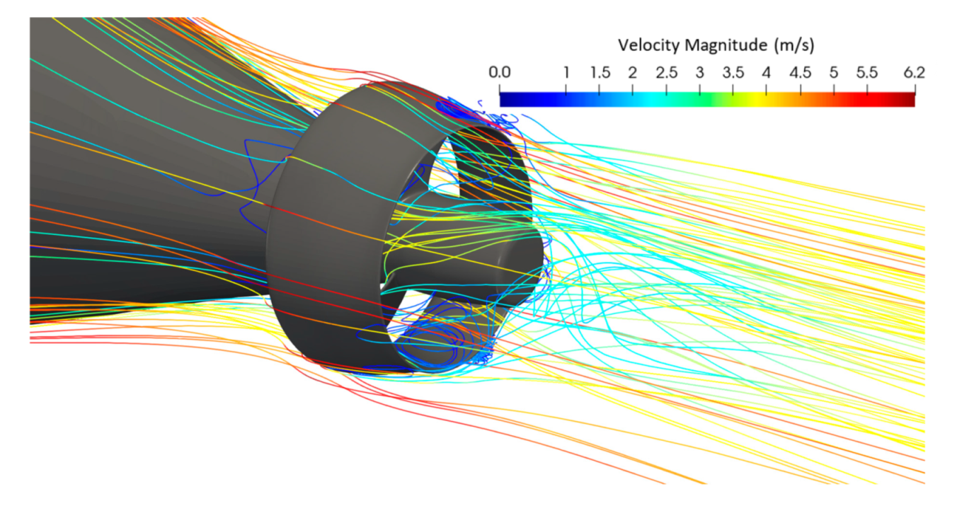
4. Results and Discussion
5. Conclusions
Author Contributions
Funding
Institutional Review Board Statement
Informed Consent Statement
Data Availability Statement
Acknowledgments
Conflicts of Interest
References
- Equinor. Subsea shuttle system. Res. Discl. 2019, 662093. [Google Scholar]
- Ellingsen, K.E.; Ravndal, O.; Reinås, L.; Hansen, J.H.; Marra, F.; Myrhe, E.; Dupuy, P.M.; Sveberg, K. Subsea shuttle system. Res. Discl. 2020, 677083. [Google Scholar]
- Xing, Y.; Ong, M.C.; Hemmingsen, T.; Ellingsen, K.E.; Reinås, L. Design Considerations of a Subsea Shuttle Tanker System for Liquid Carbon Dioxide Transportation. J. Offshore Mech. Arct. Eng. 2021, 143, 045001-1. [Google Scholar] [CrossRef]
- Ma, Y.; Xing, Y.; Ong, M.C.; Hemmingsen, T.H. Baseline design of a subsea shuttle tanker system for liquid carbon dioxide transportation. Ocean. Eng. 2021, 240, 109891. [Google Scholar] [CrossRef]
- Kretschmann, L.; Burmeister, H.-C.; Jahn, C. Analyzing the economic benefit of unmanned autonomous ships: An exploratory cost-comparison between an autonomous and a conventional bulk carrier. Res. Transp. Bus. Manag. 2017, 25, 76–86. [Google Scholar] [CrossRef]
- CCSA. What Is CCS? Available online: http://www.ccsassociation.org/what-is-ccs/ (accessed on 30 December 2019).
- IEA. Energy Technology Perspectives 2010: Scenarios and Strategies to 2050; OECD Publishing: Paris, France, 2010. [Google Scholar]
- Weller, H.G.; Tabor, G.; Jasak, H.; Fureby, C. A tensorial approach to computational continuum mechanics using object-oriented techniques. Comput. Phys. 1998, 12, 620–631. [Google Scholar] [CrossRef]
- Katsui, T.; Kajikawa, S.; Inoue, T. Numerical investigation of flow around a ROV with Crawleer based driving system. In Proceedings of the ASME 2012 31st International Conference on Ocean, Offshore and Arctic Engineering, Rio de Janeiro, Brazil, 1–6 July 2012. [Google Scholar]
- Shang, Z.; Emerson, D.; Gu, X. Numerical investigations of cavitation around a high speed submarine using openfoam with les. Int. J. Comput. Methods 2012, 9, 1250040. [Google Scholar] [CrossRef]
- Jones, D.A.; Chapuis, M.; Liefvendahl, M.; Norrison, D.; Widjaja, R. RANS Simulations Using OpenFOAM Software; DST-Group-TR-3204 Report; Maritime Platforms Division, DST Group Defence Science and Technology Group: Canberra, Australia, 2016. [Google Scholar]
- Fureby, C.; Anderson, B.; Clarke, D.; Erm, L.; Henbest, S.; Giacobello, M.; Jones, D.; Nguyen, M.; Johansson, M.; Jones, M.; et al. Experimental and numerical study of a generic conventional submarine at 10° yaw. Ocean Eng. 2016, 116, 1–20. [Google Scholar] [CrossRef]
- Xing, Y. A Conceptual Large Autonomous Subsea Freight-Glider for Liquid CO2 Transportation. In Proceedings of the Volume 6: Ocean Engineering, ASME International, Virtual, Online, 21–30 June 2021. [Google Scholar]
- Ellingsen, K.E.; Equinor, Stavanger, Norway. Personal Communication, 2019.
- OpenFoam. The Open Source CFD Toolbox, User Guide v1812. 2018. Available online: https://www.openfoam.com/documentation/user-guide (accessed on 25 March 2020).
- ASME. ASME V V 20: Standard for Verification and Validation in Computational Fluid Dynamics and Heat Transfer; ASME: New York, NY, USA, 2009. [Google Scholar]
- Jones, M.B.; Erm, L.P.; Valiyff, A.; Henbest, S.M. Skin Friction Measurements on a Model Submarine; DSTO Report; Aerospace Division, Defence Science and Technology Organisation: Canberra, Australia, 2011. [Google Scholar]
- Stefes, B.; Fernholz, H.-H. Skin friction and turbulence measurements in a boundary layer with zero-pressure-gradient under the influence of high intensity free-stream turbulence. Eur. J. Mech.-B/Fluids 2004, 23, 303–318. [Google Scholar] [CrossRef]
- Zarastvand, M.R.; Ghassabi, M.; Talebitooti, R. Acoustic Insulation Characteristics of Shell Structures: A Review. Arch. Comput. Methods Eng. 2021, 28, 505–523. [Google Scholar] [CrossRef]
- Asadijafari, M.; Zarastvand, M.; Talebitooti, R. The effect of considering Pasternak elastic foundation on acoustic insulation of the finite doubly curved composite structures. Compos. Struct. 2021, 256, 113064. [Google Scholar] [CrossRef]


| Main Design Parameter | Value |
|---|---|
| Maximum water depth | 350 m |
| Minimum water depth | 200 m |
| Operating speed, U | 6 knots (3.09 m/s) |
| Length, L | 135 m |
| Diameter, D | 17 m |
| Water temperature, T | 4 °C |
| Kinematic viscosity of water at 4 °C, ν | 1.626 × 10⁻⁶ m2/s |
| Maximum current velocity | 1 m/s |
| Reynolds number, ReL | 3.398 × 10⁸ |
| Parameter | Value |
|---|---|
| Time discretization | Crank–Nicolson, second order |
| Gradient discretization | Gauss linear, second order |
| Divergence discretization | Gauss linear, second order |
| Laplacian discretization | Linear with nonorthogonal correction, second order |
| Cell-to-face interpolation | Linear, second order |
| Surface normal gradient discretization | Linear with nonorthogonal correction, second order |
| Pressure linear solver | Preconditioned Conjugate Gradient |
| Pressure solver tolerance | 10−6 |
| Velocity, k, and ω linear solver | Smooth solver with Gauss–Seidel smoother |
| Velocity solver tolerance | 10−8 |
| Mesh Variant | Number of Cells |
|---|---|
| M1 Coarse | 4.2 million |
| M2 Medium | 9.8 million |
| M3 Dense | 19.6 million |
| M1 Coarse | M2 Medium | M3 Dense | |
|---|---|---|---|
| Total drag force FD [kN] | 244.47 | 226.08 | 221.97 |
| Relative error [%] | 10.13 | 1.85 | - |
| Pressure drag component FD, Pressure [kN] | 152.07 | 131.35 | 126.66 |
| Relative error [%] | 20.07 | 3.7 | - |
| Viscous drag component FD, Viscous [kN] | 92.40 | 94.74 | 95.31 |
| Relative error [%] | 3.06 | 0.61 | - |
Publisher’s Note: MDPI stays neutral with regard to jurisdictional claims in published maps and institutional affiliations. |
© 2021 by the authors. Licensee MDPI, Basel, Switzerland. This article is an open access article distributed under the terms and conditions of the Creative Commons Attribution (CC BY) license (https://creativecommons.org/licenses/by/4.0/).
Share and Cite
Xing, Y.; Janocha, M.J.; Yin, G.; Ong, M.C. CFD Investigation on Hydrodynamic Resistance of a Novel Subsea Shuttle Tanker. J. Mar. Sci. Eng. 2021, 9, 1411. https://doi.org/10.3390/jmse9121411
Xing Y, Janocha MJ, Yin G, Ong MC. CFD Investigation on Hydrodynamic Resistance of a Novel Subsea Shuttle Tanker. Journal of Marine Science and Engineering. 2021; 9(12):1411. https://doi.org/10.3390/jmse9121411
Chicago/Turabian StyleXing, Yihan, Marek Jan Janocha, Guang Yin, and Muk Chen Ong. 2021. "CFD Investigation on Hydrodynamic Resistance of a Novel Subsea Shuttle Tanker" Journal of Marine Science and Engineering 9, no. 12: 1411. https://doi.org/10.3390/jmse9121411
APA StyleXing, Y., Janocha, M. J., Yin, G., & Ong, M. C. (2021). CFD Investigation on Hydrodynamic Resistance of a Novel Subsea Shuttle Tanker. Journal of Marine Science and Engineering, 9(12), 1411. https://doi.org/10.3390/jmse9121411