Article

Technical–Economic Feasibility Analysis of Subsea Shuttle Tanker

Department of Mechanical and Structural Engineering and Materials Science, University of Stavanger, 4021 Stavanger, Norway
*
Author to whom correspondence should be addressed.
J. Mar. Sci. Eng. 2022, 10(1), 20; https://doi.org/10.3390/jmse10010020
Submission received: 22 November 2021 / Revised: 15 December 2021 / Accepted: 23 December 2021 / Published: 26 December 2021
(This article belongs to the Special Issue Instability and Failure of Subsea Structures)

Abstract

:
This paper presents the technical and economic feasibility analysis of the subsea shuttle tanker (SST). The SST is proposed as an alternative to subsea pipelines and surface tankers with the primary purpose of transporting CO2 autonomously underwater from onshore facilities to subsea wells for direct injection at marginal subsea fields. In contrast to highly weather-dependent surface tanker operations, the SST can operate in any condition underwater. The technical–economic analysis is performed in two steps. First, the SST’s technical feasibility is evaluated by investigating designs with lower and higher capacities. The purpose is to observe the appearance of technical limits (if present) when the SST is scaled down or up in size. Second, an economic analysis is performed using the well-reviewed cost models from the publicly available Zero Emissions Platform (ZEP) and Maritime Un-manned Navigation through Intelligence in Networks (MUNIN) D9.3 reports. The scenarios considered are CO2 transport volumes of 1 to 20 million tons per annum (mtpa) with transport distances of 180 km to 1500 km in which the cost per ton of CO2 is compared between offshore pipelines, crewed/autonomous tanker ships, and SST. The results show that SSTs with cargo capacities 10,569 m3, 23,239 m3, and 40,730 m3 are technically feasible. Furthermore, the SSTs are competitive for short and intermediate distances of 180–750 km and smaller CO2 volumes of 1–2.5 mtpa. Lastly, it is mentioned that the SST design used the DNVGL Rules for Classification for Naval Vessels, Part 4 Sub-surface ships, Chapter 1 Submarine, DNVGL-RU-NAVAL-Pt4Ch1, which is primarily catered towards military submarine design. It is expected that a dedicated structural design code that is optimized for the SST would reduce the structural weight and corresponding capital expenditure (CAPEX).

1. Introduction and Background

Most offshore oil and gas transportation from shore is accomplished using pipelines [1]. Since the first submerged pipeline was installed in the United Kingdom during World War II, subsea pipeline laying methods have improved enormously and are currently regarded as a well-established technology [2]. At present, there are several technical and economic restrictions for this mode of transportation. An important drawback is the high cost of deployment, which leads to it being prohibitively expensive for distant oil and gas fields, as costs increase exponentially as pipeline lengths rise. Aside from that, deep-water inspections for pipelines may also be demanding and costly. Further, pipeline maintenance and repair may require a whole or partial shutdown and may not be ideal from a cost perspective. It is normally not economical to use offshore pipelines at a remote marginal field. In this case, shuttle tanker ships1 are often utilized [3]. It is more attractive to employ a pipeline when the operations have minimal step-outs and high-profit margins, which is normally the case for large fields [4]. A tanker ship is also a flexible option because it may be quickly deployed to many fields under most circumstances. In some cases, it is advantageous to use tanker ships instead of offshore pipelines, as a replacement tanker may be sent quickly in the event of a problem. However, tanker ship operations are weather-dependent and can be difficult to conduct in adverse weather circumstances because of the large dynamic load-effects from the environment (i.e., wind and wave action). On that the account, Subsea Shuttle Tanker (SST) concept was introduced as a potential alternative to subsea pipelines and tankers in order to overcome the limitations mentioned above [5,6,7,8].

1.1. Previous Research in Underwater Cargo Vessels

The idea of using underwater vessels for commercial transportation is not new. In the 1970s, Jacobsen [9] and Taylor et al. [10] proposed using nuclear-powered submarines of various sizes, 20,000 to 420,000 dead weight ton (DWT), to transport Arctic crude oil. In the 1980s, Jacobsen et al. [11] proposed two giant Arctic Liquefied Natural Gas (LNG) submarine tankers, 660,000 DWT nuclear-powered and a 727,400 DWT conventionally-powered submarines. In two research disclosures by Equinor [5,6], a sizeable autonomous cargo submarine was proposed to transport CO2, hydrocarbon, and subsea tools. In the latter research disclosure, Ellingsen et al. [6] also proposed an innovative maritime freight option, a subsea ‘cargo train’ made up of interconnected subsea train-like tanks with independent propulsion units located at the vessel bow or aft. Further, Ellingsen et al. [6] also proposed an ultra-efficient large subsea transport glider. Based on that, Xing [12] proposed a 785 DWT subsea cargo glider with a calculated average power consumption of below 10 kW. In general, the works mentioned above did not go beyond conceptual design proposals. Xing et al. [7] and Ma et al. [8] closed this knowledge gap by considering the most critical design considerations and defining a baseline SST design that entails detailed global design specifications.

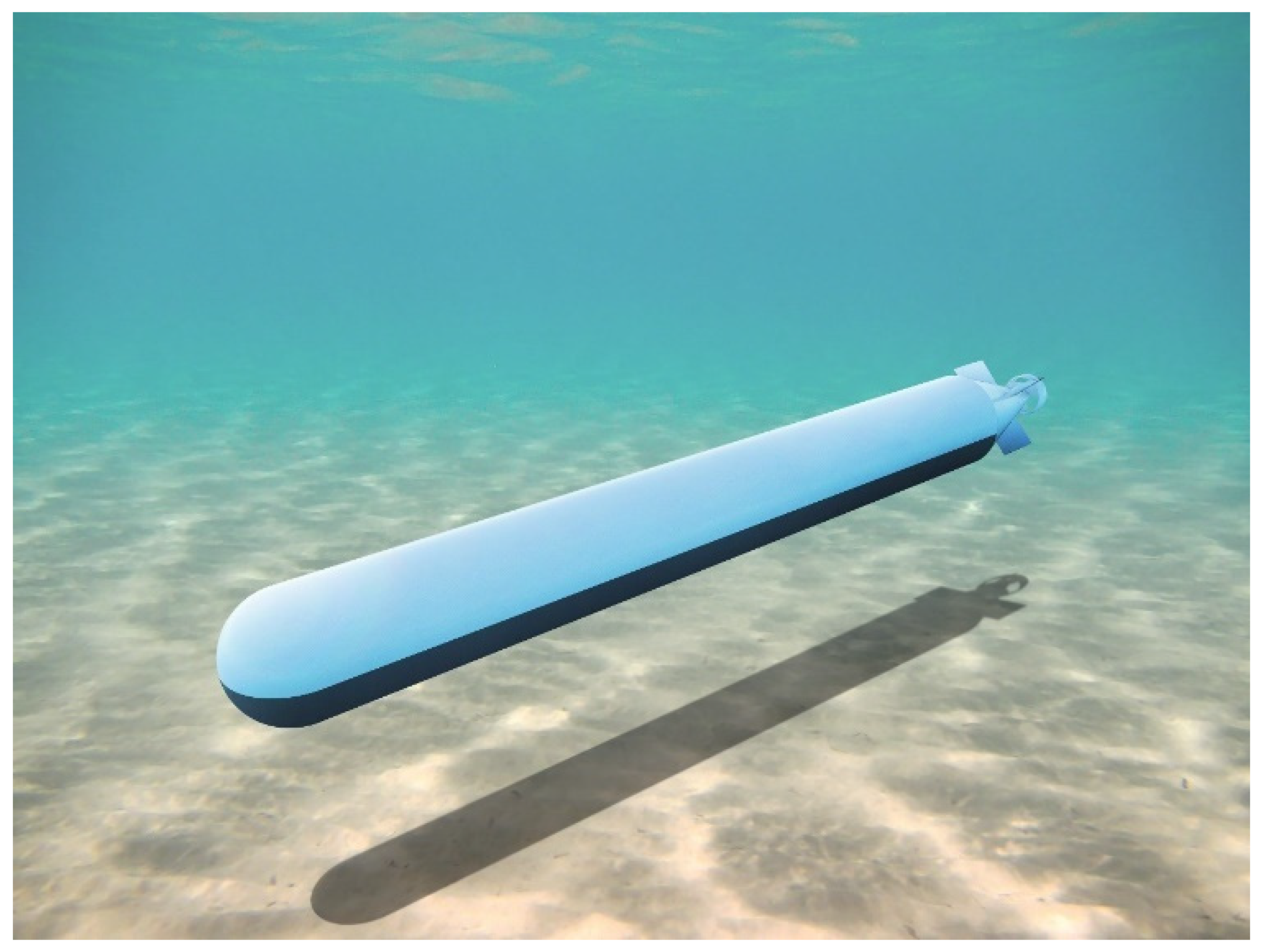
1.2. The Subsea Shuttle Tanker (SST)

The SST is an offshore submersible transportation vessel that can operate in any weather conditions. The SST is presented in Figure 1 and is designed with the primary purpose of transporting CO2 autonomously underwater from onshore facilities to subsea wells for direct injection. The SST baseline design [8] was designed for the Norwegian Continental Shelf, where three Carbon Capture and Storage (CCS) projects are presently operating: Sleipner, Utgard, and Snøhvit [13]. At present, CO2 generated during hydrocarbon production is caught and reinjected into the reservoir in these operations. Further, along with these three current projects, the Northern Lights project [14] will begin operations in 2024 and transport CO2 produced by non-petroleum-related industrial activities to the Troll field for injection into the Utsira formation. Figure 2 illustrates the locations of these CCS projects. Even though the SST was originally designed for these CCS projects, it can be configured to operate in other locations across the globe. Furthermore, it has been mentioned that the baseline SST design [8] allows for more detailed studies of the SST concept which have yet to be performed. Some examples include Ma et al. [15,16,17] and the study presented in this paper.
Figure 3 illustrates the three transportation methods considered in this paper, offshore pipelines, tanker ships, and SST. The capture source normally holds CO2 at 110 bar and 40 °C. The CO2 must be processed at different pressures and temperatures depending on the transportation method. CO2 tanker ships are generally of the semi-refrigerated or refrigerated type and transport liquid CO2 at 7 bar and −55 °C. This means that onshore liquefaction and buffer storage are required. Offshore pipelines transport CO2 in the supercritical state, with transportation pressures that are normally above 200 bar. This means that pumps are required to increase CO2 pressures from the capture source. The SST instead transports CO2 in the saturated liquid form at 35–55 bars and 0–20 °C (environmental temperature). Therefore, liquefaction and pressure boosting pumps are not required. The temperature of CO2 in the SST is be passively regulated with the surrounding environment, i.e., the CO2 is in the saturated state. This is a major advantage, as the energy required for CO2 processing is greatly reduced.
Driven by rising energy demand, CO2 concentration in the atmosphere is expected to double by 2100 compared to 1960 levels [18]; the SST can contribute to mitigation of this in various ways. The SST can assist in reducing CO2 emissions from shipping, which contributes about 3.3% of all CO2 emissions [19]. Furthermore, using marginal subsea resources to store CO2 can help to meet the future growing CCS demand [20] and increase the worldwide availability of CCS storage.
This paper performs a detailed technical and economic feasibility study on the SST. First, a technical feasibility analysis (Section 2) is performed by creating new SST designs based on the baseline SST design [8] with lower and higher cargo volumes. The rationale is to observe technical limits (if present) when the SST is scaled down or up in size. Next, an economic analysis (Section 3) is performed using the well-reviewed economic assessment methods found in the Zero Emissions Platform (ZEP) [21] and Maritime Unmanned Navigation through Intelligence in Networks (MUNIN) D9.3 [22] reports. The aim is to provide an increased understanding of the SST for its potential adoption as a critical technology for facing climate challenges. To the authors’ best knowledge, this paper presents the first publicly available detailed technical–economic analysis of a novel cargo submarine, the SST, used for CO2 transportation. The methodology presented here is relevant for other innovative large subsea cargo drone concepts such as the subsea freight-glider [12]. The economic analysis present in this paper sets the stage and provides the inputs to perform sustainability assessments that consider the wider maritime transportation value chain, such as studies on the sustainability of port regions [23,24,25], enabling the future development of zero-emission and zero-pollution maritime ports.

2. Technical Feasibility Analysis

The baseline SST design [8] is a 33,619-ton submarine with a length of 164 m and a beam of 17 m. It can carry up to 16,326 m3 of CO2 for a range of up to 400 km when travelling at a speed of 6 knots. New designs with lower and higher capacities can be created to evaluate the SST’s technical feasibility. For this analysis, half- and double-scaled versions of the baseline SST are created. These sizes are sensitivity case studies, and the purpose is to observe the appearance of technical limits (if present) when the SST is scaled down or up in size. The design methodology is presented in Figure 4 and is described briefly as follows. The design starts from the definition of the mission requirements and corresponding SST specifications (Section 2.1). The mission requirements include the operating depth, operating range, cargo capacity, and environmental data. The mission requirements will consequently define the SST specifications, which include properties of the CO2 cargo, expected load effects, required speed, and range. The general arrangement (Section 2.2) defines the location of each component in the SST. The baseline SST general arrangement is used for all SSTs created. The structural calculations are performed for the external and internal hulls based are then calculated using information from the SST specifications and general arrangement (Section 2.3). The structural design is based on the state-of-art engineering codes and standards, DNV-RU-NAVAL-Pt4CH1 [26] and American Society of Mechanical Engineers Boilers and Pressure Vessel Code ASME BPVC VIII-2 [27]. The hydrostatic check is performed thereafter (Section 2.4). The design will be iterated if the check is not passed, i.e., the dimensions are adjusted. The power consumption is estimated if a design is obtained (Section 2.5). Full details of the design procedure can be found in Ma et al. [8].
The target percentage payload is 50% displacement. This is achieved by employing a double hull design with active pressure compensating systems that limit the external pressure loads on the external pressure hull structures. In doing so, the external hull need not be designed for the full hydrostatic pressure at the water depth it is operating in. Further details of this system can be found in Xing et al. [7] and Ma et al. [8]. This 50% payload target is maintained for all sizes of the SST created in this paper. Further, for a fair comparison, the SSTs are designed with the same safety factor.

2.1. Mission Requirements and SST Specifications

This section defines and discusses the mission requirements and SST specifications, which serve as the foundation for the design. The baseline SST operating specifications are summarized in Table 1.
A safety depth of 40 m is used to prevent collisions with surface ships or floating facilities. This depth also reduces the dynamic load effects from waves and leads to the SST being weather-independent. The SST is designed to transport CO2 at a constant 70 m nominal diving depth, which is defined based on the minimum recoverable depth from loss of control. The test diving depth is 105 m, which is defined as 1.5 times the nominal diving depth. Further, the collapse depth is 190 m, which is 2.7 times the nominal diving depth. These depths are defined in accordance with Table 1 in DNV-RU-NAVAL-Pt4CH1 [26]. The operating depth range of the SST, therefore, is between 40 m (safety depth) and 70 m (nominal diving depth).
The baseline SST has a range of 400 km, which allows it to travel back and forth between Snøhvit and Troll or one way between Sleipner and Utgard. For a fair comparison, the technical feasibility analysis uses 400 km as the range for every SST design. Note that the payload will be reduced correspondingly by the increased battery weight required for the distances of 500 km, 750 km, and 1500 km used in the economic analysis (Section 3). However, this reduction is negligible as the battery weight is only 40 tons and is only a small portion of the total weight of 33,619 tons for the baseline SST.
The baseline SST has a cargo capacity of 15,000 tons, which allows transporting of an annual CO2 volume of 1.5 million tons with two trips per week. The half- and double-scale SST can transport approximately half and double cargo compared to the baseline SST, respectively.
The baseline SST can operate in environment ambient temperatures between 0 °C and 20 °C. As a reference, the seawater temperature is 2–12 °C in the Norwegian sea (0–10° E, 60–70° N) [28]. The current design speed is 1 m/s, which represents the highest seasonal average current speed of the North Atlantic current and Norwegian coastal current; the observed seasonal average current speed in the Norwegian sea is around 0.2 m/s [29,30,31].

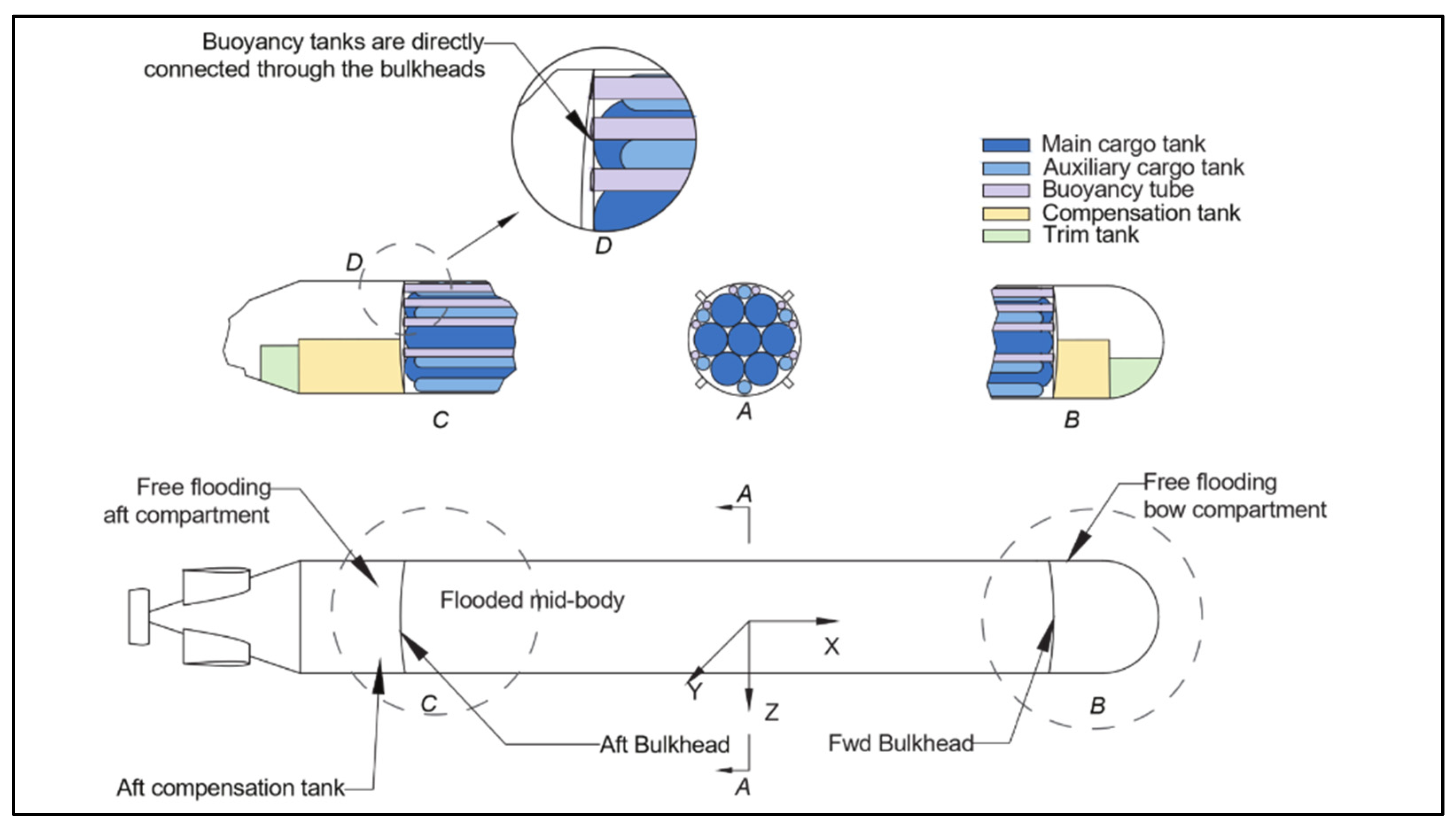
2.2. General Arrangement

The general arrangement is shown in Figure 5 and shows the external hull compartments and internal tanks. The SST uses a torpedo-shaped external hull for low drag resistance. The external hull consists of a hemispherical bow, a cylindrical mid-body, and a conical aft. The bow and aft portions are about 23% of the total steel external hull weight in the baseline SST. A double hull design is utilized at the cylindrical mid-body to avoid the need for a collapse pressure design. This means that the mid-body external hull does not experience any hydrostatic pressure differential loading. The smaller internal pressure hulls (cargo tanks and buoyancy tubes) are designed to handle both burst and collapse pressures. The SST has four bulkheads, which are used to separate the flooded mid-body from the free flooding compartment and to support the internal cargo tanks and buoyancy tubes.
The SST external hull consists of three compartments: (i) a free flooding aft compartment, which holds moisture-sensitive equipment (gearbox, motor, battery, aft trim tank, aft compensation tank, and rudder controls); (ii) a free flooding bow compartment which holds sonar, radio, sensors, control station, forward compensation and trim tanks, and pumps for offloading; and (iii) a flooded mid-body in the middle, which is the largest compartment and holds buoyancy tanks, cargo tanks, and piping. There are five types of internal pressure vessels in the SST, the main cargo tank, auxiliary cargo tank, buoyancy tube, compensation tank, and trim tank.
  • Cargo tanks: There are seven main cargo tanks and six auxiliary cargo tanks with hemispherical ends, distributed circular-symmetrically in the SST’s flooded mid-body.
  • Compensation tanks: There are two compensation tanks to provide the vessel with the trimming moment and weight necessary to reach neutral buoyancy under different hydrostatic load cases. These tanks are used to ensure the neutral buoyancy of the SST under different load cases.
  • Trim tanks: Two trim tanks are in the bow hemisphere and aft cone of the SST. These tanks bring the centre of gravity (CoG) vertically beneath the centre of buoyancy (CoB) so that the vessel is at a neutral trim condition. The trim tanks do not communicate with the open sea and only handle internal pressure resulting from hydrostatic pressure.
  • Buoyancy tubes: Eight empty buoyancy tanks are arranged at the upper part of the SST to make the vessel neutral buoyant. These buoyancy tanks are of the same length as the main cargo tanks and are directly connected to the forward and aft bulkheads.
  • The main cargo tanks, auxiliary cargo tanks, compensation tanks, and trim tanks are designed to take burst pressure, while the buoyancy tubes are designed against collapse pressure.

2.3. Structural Design

2.3.1. Materials

Table 2 presents the materials and corresponding properties used in the SST structures.

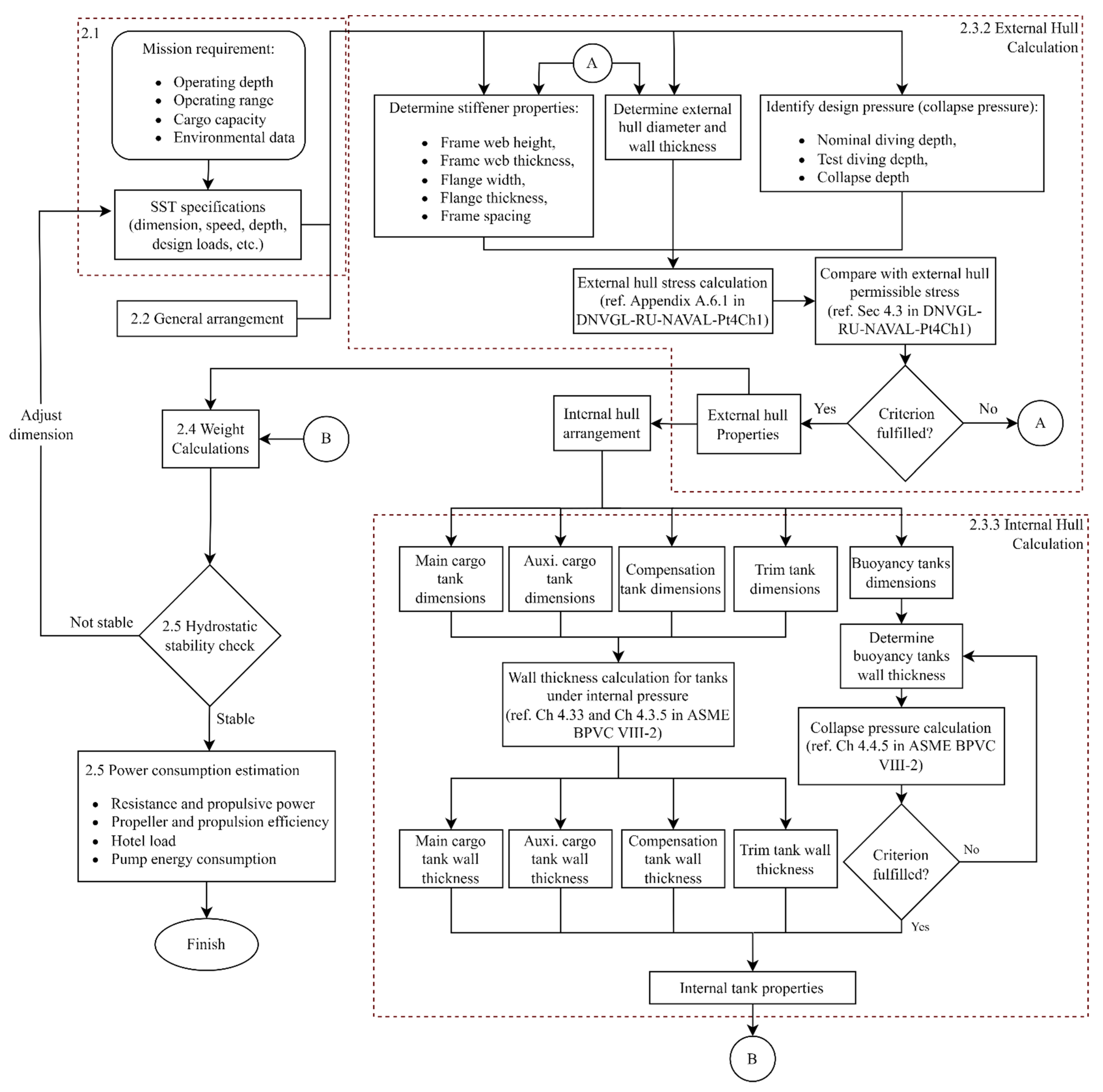
2.3.2. External Hull Design

The SST uses a torpedo-shaped hull with a slenderness ratio (diameter vs length) of 1:9.7. The design was selected because its geometrical simplicity and slenderness ratio are optimized between minimum drag resistance and cargo volume. The external hull compartments are as follows.
  • Free flooding compartments are pressure hulls subjected to hydrostatic pressures. These compartments are checked against permissible stress at the nominal diving depth, test diving depth, and collapse depth in accordance with Chapter 4 in DNVGL Rules for Classification for Naval Vessels, Part 4 Sub-surface ships, Chapter 1 Submarine (DNVGL-RU-NAVAL-Pt4Ch1) [26].
  • The flooded mid-body compartment is designed with the same reference as the free flooding compartments. However, this part of the external hull does not handle hydrostatic pressure. Hence, it uses 7 bar (70 m) for collapse pressure to prevent immediate structural failure in accidental load cases, such as mid-body seawater vent malfunction.
  • The bulkhead is designed using a finite element analysis and uses permissible stresses in DNVGL-RU-NAVAL-pt4Ch1 Section 4.3 [26]. The permissible stress in the nominal diving depth check is 203 MPa, in the test diving depth is 418 MPa, and in the collapse depth check is 415 MPa.
  • The stiffener properties used for the external hull are presented in Table 3. The external hull uses stiffeners in accordance with the calculation method in DNV-RU-NAVAL-Pt4Ch1 [26].
Table 3. Stiffener properties.
ParameterSymbolUnitsValue
Frame web heighthw(m)0.3
Frame web thicknesssw(m)0.03
Flange widthbf(m)0.1
Flange thicknesssf(m)0.033
Frame spacingLF(m)1
Frame cross sectional areaAF(m)0.0123
Inner radius to the flange of the frameRf(m)6.1380
The SST external hull designs are presented in Table 4. In general, the external hull’s mid-body is the biggest part and accounts for 54% of its baseline SST’s structural weight.
The detailed external hull design calculations for the half-scaled SST (10,569 m3) are presented in the first part of Appendix A.

2.3.3. Internal Hull Design

The internal tanks are designed in accordance with ASME BPVC Chapter 4, Section VIII, Division 2 [27]. The internal tanks are described in the following:
  • Cargo tanks are subjected to external hydrostatic pressure and internal tank pressure. They are used for CO2 storage and have a design burst pressure of 55 bar. This is identified as the worst-case scenario, which occurs when the SST is floating on the sea surface. Under this condition, the external hydrostatic pressure is 0 bar gauge, and the pressure difference is 55 bar. The cargo tanks avoid collapse pressure design by utilizing a pressure compensation system (PCS). Details of the PCS are provided in Xing et al. [7] and Ma et al. [8]. The different diameters allow for a more optimal arrangement of the tanks within the SST, thereby maximizing space utilization and consequently payload.
  • Compensation and trim tanks are soft tanks in the free flooding compartments, i.e., they do not need to handle external pressure. Consequently, they only need to handle internal pressure, which results from the hydrostatic pressure due to the flooding of the mid-section in the SST. During the calculation, compensation tanks and trim tanks are assumed to be cylindrical to obtain reasonable weight and volume sizing. They can, however, be made of various shapes to better utilize the space in the free flooding compartments.
  • Buoyancy tanks are designed to handle 7 bar hydrostatic pressure, corresponding to the 70 m nominal diving depth.
  • The SST internal tank designs are presented in Table 5.
The detailed internal tank design calculations for the half-scaled SST (10,569 m3) are presented in the second part of Appendix A.

2.4. Weight Calculations

The weights and weight compositions of the SSTs are calculated after a structural design (Ref. Section 2.3) is completed. The following definitions are used for all SSTs:
  • The targeted payload is 45% displacement
  • The machinery weight is 3% displacement
  • The permanent ballast is 3% displacement
  • The trim ballast is 0.7% displacement
The weights and weight compositions for the CO2-filled condition (Section 2.5) are presented in Table 6.

2.5. Hydrostatic Stability Check

The hydrostatic stability of the SST is checked against the criteria in DNVGL-RU-NAVAL-Pt4Ch1, Section 3.5.2.3 [26] for submarines exceeding 2000 DWT in the submerged condition and surfaced condition. The SST’s distance between the centres of buoyancy (B) and gravity (G) must exceed 0.35 m. Further, the relative position of metacentric height (GM) must be greater than 0.22 m. There are four hydrostatic load cases considered, as follows. (i) Submerged (CO2-filled): the SST is fully loaded and submerged, with all 13 tanks filled with liquid CO2. (ii) Submerged (SW-filled): the SST has just offloaded its CO2 at the well, and the vessel is submerged with all 13 tanks filled with seawater. (iii) Surfaced (CO2-filled): the vessel is floating on the surface with all 13 tanks filled with liquid CO2; this situation occurs when the SST is loading at the port. (iv) Surfaced (SW-filled): the vessel is floating on the surface with five main tanks and three auxiliary tanks at the bottom filled with seawater ballast; the remaining tanks are empty. This situation occurs when the SST returns to the port after its journey. More details about the hydrostatic checks can be found in Ma et al. [8]. The results from the hydrostatic checks are summarized in Table 7.

2.6. Power Consumption Estimation

The total power consumption with a transport speed of 6 knots and distance of 400 km for SSTs with volumes 10,569, 23,239, and 40,730 m3 are 358,764, 620,249, and 955,292 kW, respectively. These are calculated based on the resistance power of the subsea shuttle tanker towards the forces of the water current, propulsive power, hotel load, and pump energy consumptions. Each different design parameter is adjusted based on the needs of the design. The power consumption curves are presented in Figure 6 and are calculated based on the following.
  • The resistance power is based on the skin friction obtained from the International Towing Tank Conference-57 correlation line [32], and the drag pressure is obtained empirically from Hoerner’s scheme [33].
  • The propulsive power is calculated with three-bladed Wageningen B-series for the propeller [34], and the corresponding quasi-propulsive coefficients (QPC) are between 0.8 until 1.0 [35]. The torque coefficient, thrust coefficient, and propulsion efficiency are 0.01, 0.17, and 0.88, respectively.
  • The hotel load power consumption is estimated from existing tanker ships from Wärtsilä [36], with a 40% reduction to account for the fact that the SST is autonomous and operates without any crew [37].
  • The pump power is estimated from the duration of the pump flow to load and offload the cargo. The pumps provide 3 bar differential pressure and take 4 hours to transfer the cargo. This means that every SST design has different pump volumetric flow rates to ensure the same offloading duration. The pump efficiency is defined to be 75% [38,39].
Li-ion battery is chosen for the SST for its steady power output and high capacity. It has the capacity of the half-scale and baseline SST uses a 20,000 kWh and a 40-ton battery, while the double-scale SST uses 40,000 kWh and an 80-ton battery.

2.7. Derived Designs

The main parameters of the final derived designs are presented in Table 8.

3. Economic Feasibility

The economic analysis uses the well-reviewed cost models from the publicly available ZEP [21] and MUNIN D9.3 [22] reports. The ZEP report [21] presents the study of CO2 transport costs performed by ZEP, who serve as the technical advisor to the EU commission on the deployment of CCS and carbon capture and utilization (CCU). The ZEP report [21] is based on consensus-based data provided by member organizations, including key stakeholders such as Gassco, Teekay Shipping, and Open Grid Europe. These are the most prominent players in maritime transport. The cost analysis is detailed to the component level. For example, the cost of coating for the offshore pipeline is defined and considered. This paper, in general, primarily uses the cost models from the ZEP report. The MUNIN D9.3 report [22] presents a detailed analysis of the autonomous ship developed in the MUNIN project in the areas of safety and security impacts, economic impacts, and applicable areas of law. The cost analysis used for the economic impact assessment is also very detailed, and the data related to autonomous ships are used in this paper. Similar to the ZEP report, the MUNIN D9.3 report uses consensus-based data provided by key players in the maritime transport industry. A summary of the cost models used in the ZEP [21] and MUNIN D9.3 [22] reports is presented in Table 9.
The scenarios considered are CO2 transport volumes of 1, 2.5, 10, and 20 million tons per annum (mtpa) with transport distances of 180, 500, 750, and 1500 km. The CO2 is assumed to be delivered from the capture plant at 110 bar and ambient temperature. Further, the following CO2 transport assumptions are used. The cost of the subsea well-head template is not considered. Ship transport and SST discharge directly to the well without the use of intermediate buffer storage. More than one transport vessel is required in some scenarios due to the long distances and/or large CO2 volumes. For example, in the 2.5 mtpa transport volume and 500 km distance scenario, the two 23,239 m3 SST are required, while only one SST is required if the 40,730 m3 version is used. The interest rate applied for all assessments is the same as for the other part of the CCS chain, 8%, with a project lifetime is 40 years. The costs refer to cost levels in the third quarter of 2021. The currency exchange rates used are 0.87 EUR/USD.
The economic analysis details for the offshore pipelines, crewed/autonomous tanker ships and SST are presented in Section 3.1, Section 3.2 and Section 3.3, respectively. The economic calculations for the 180 km and 2.5 mtpa case are presented in Appendix B.

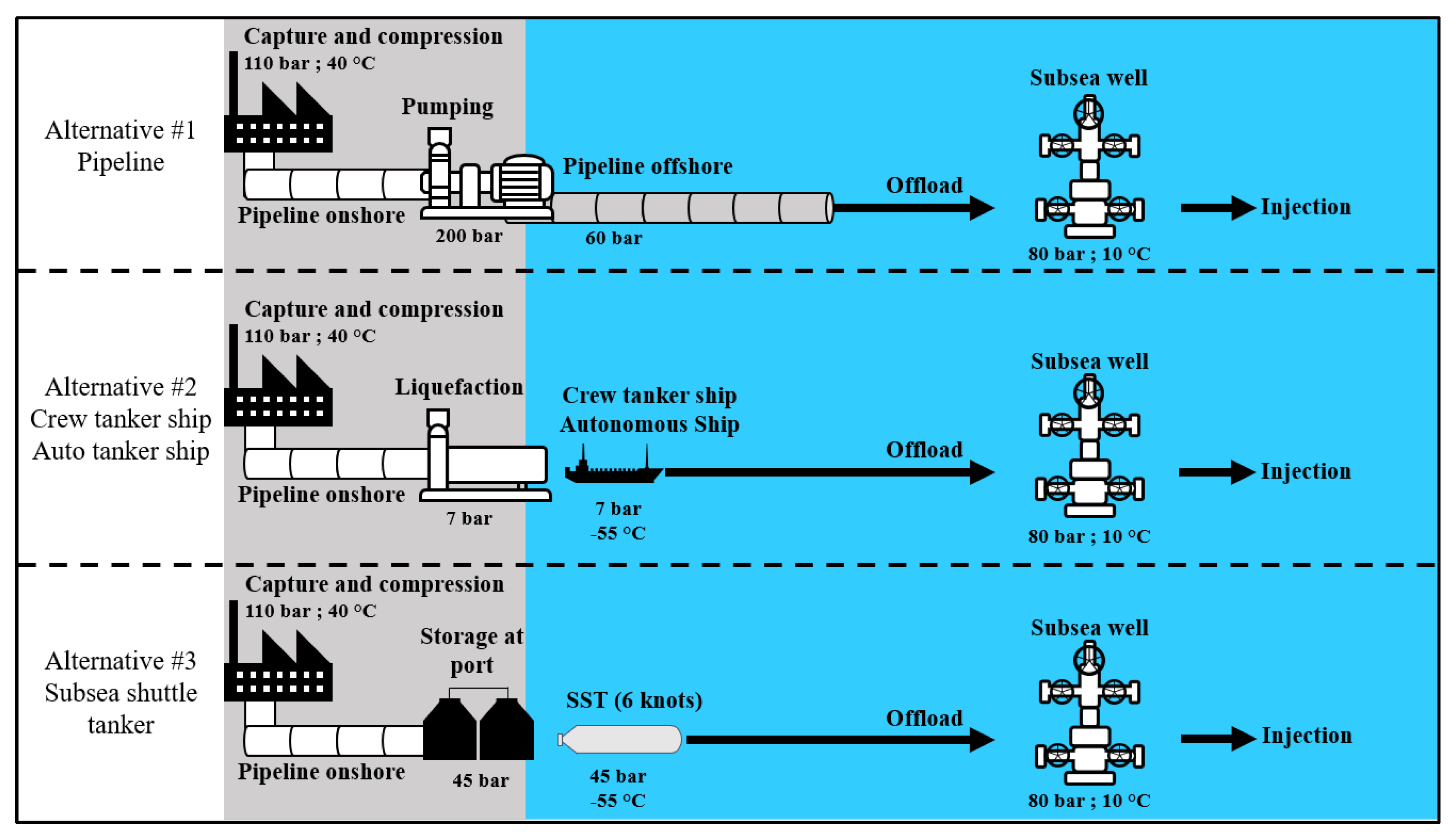
3.1. Offshore Pipelines

In general, offshore pipeline costs are mainly determined by CAPEX and are roughly proportional to distance. They therefore benefit significantly from economies of scale and full capacity utilization. The design of offshore pipelines is driven mainly by the desired transport capacity, pipeline dimensioning (diameter), inlet and outlet pressure, steel quality, and pipeline wall thickness. Other factors such as the pipeline route along the seabed, on-bottom stability, corrosion protection, dropped object protection, design against trawling, and installation method are also important.
The CAPEX is estimated based on the market steel price, coating (anti-corrosion/weight), pipeline installation cost, and trenching. The costs of the manifold for the well and drilling of the injection wells are not included in these costs. CO2 is transported in the supercritical phase (55–88 bar), which requires the use of pressure boosters, and the corresponding costs are included in the pipeline CAPEX. In addition, the pressure of the CO2 in the pipeline is dependent on conditions in the geological storage site. In this study, the costs for the compression of the CO2 up to 110 bars before transport are included in the cost of the capture plant.
The pipeline route considered starts at the Belgian coast and ends at the Norwegian continental shelf. The starting point is close to heavily industrialized areas in Europe, and the routing is in the proximity of several promising storage areas. Thus, the cases described through this route may be representative of possible future transport solutions. Further, it is mentioned that the lowest volume case of 1 CO2 mtpa is not considered. This case is not interesting for the offshore pipeline as it is well known that the offshore pipeline is not economical for low transportation volumes [40].
The properties and component pricing for the offshore pipelines are presented in Table 10 and Table 11.
Based on the above design definitions and corresponding costs, the pipeline annuities for 2.5, 10, and 20 mtpa transport volumes are 20.99–126.96 m€, 28.34–197.92 m€, and 35.54–293.60 m€, respectively. Details are presented in Table 12. The corresponding operating expenditures (OPEXs) are 2.35 m€/a, 4.76 m€/a, and 7.9 m€/a, respectively. All aspects of maintenance and operational costs are included in the OPEX.

3.2. Crewed/Autonomous Tanker Ship

CO2 tanker ships have designs such as semi-refrigerated liquefied petroleum gas (LPG) carriers, and transport gas at temperatures of −50 °C. A tanker ship requires liquefaction and refrigeration during the voyage, during which the CO2 will be transported at 7–9 bar and as low as −55 °C in order to avoid any risk of dry ice formation. An onshore liquefaction plant is required to condense and depressurize the CO2. During transport, the temperature of the CO2 will rise, causing boil off and increasing the internal vessel pressure. As a result, the cargo tank pressure at the end of the loaded voyage will normally be 8–9 bar.
The tanker ship properties are presented in Table 13.
The CAPEX is calculated based on price/ton structural steel weight. The minimum and maximum price per ton of steel derived from all ships in the ZEP report [21] are used, giving 11,631–28,888 €/ton, as presented in Figure 6 and Table 14. As presented in Figure 6, the maximum and minimum CAPEXs are extrapolated from the data presented in ZEP report [21]. The autonomous tanker ship is assumed to have a CAPEX of 110% of the crewed tanker ship. The ships are assumed to be manufactured in the Far East and are modern ships with dynamic positioning and submerged turret offloading buoy capabilities.
The OPEX inputs used are presented in Table 15. The tanker ships are assumed to be powered by LNG or conventional marine diesel oil. The price per ton is the same for these fuels. A Far Eastern crew is also used.
Based on the above definitions, the CAPEX for the crewed tanker ship is around 60–149 m€ for the size of 22,000 m3 and 112–278 m€ for the size of 41,000 m3. Correspondingly, the CAPEX for the autonomous tanker ship is around 66–164 m€ and 123–306 m€, respectively.

3.3. Subsea Shuttle Tanker

The SST’s CAPEX is calculated based on the structural weight and steel per ton price. For a fair comparison, it is assumed the SST will in the future achieve similar technical maturity and economies of scale as the tanker ship; therefore, the steel per ton price is assumed to be the same as the tanker ship. With this assumption, the SST CAPEX is calculated to be 102–254 m€, 115–286 m€, and 210–522 m€ for SST with cargo sizes of 10,569 m3, 23,239 m3, and 40,730 m3, respectively. The SST operations are assumed to also be like that of the tanker ship, and cost 2% of the CAPEX. The electricity price is assumed to be 0.11 €/kWh.

4. Results and Discussions

In this section, the results of the technical feasibility analysis and economic feasibility analysis results are discussed. To the authors’ knowledge, this paper presents the first publicly available detailed technical–economic analysis of a novel cargo submarine, the SST, used for CO2 transportation, along with comparisons to offshore pipelines and crewed/autonomous tanker ships.

4.1. Technical Feasibility

It is shown that SSTs with cargo capacities of 10,569 m3, 23,239 m3, and 40,730 m3 fulfilling the mission requirements and SST specifications can be designed using the design methodology presented in Ma et al. [8]. Therefore, the SST designs considered in this paper are technically feasible. The summary of the designs is presented in Table 8.

4.2. Economic Feasibility

4.2.1. Summary

The summary of the results presented as the transportation method with the lowest costs is presented in Table 16. The detailed results are presented in Figure 7 and Figure 8, for the mean cost per ton of CO2 and number of vessels required, respectively. In general, tanker ships have the lowest costs for longer distances, while for shorter distances with larger volumes, the offshore pipeline has the lowest costs. The SST is competitive for short and intermediate distances of 180–750 km for and for smaller CO2 volumes of 1–2.5 mtpa. The SST has the lowest cost for the smallest CO2 volumes and distances (1–2.5 mtpa and 180 km). It is also observed that the cost per ton of CO2 reduces with increasing CO2 volumes due to better economies of scale.

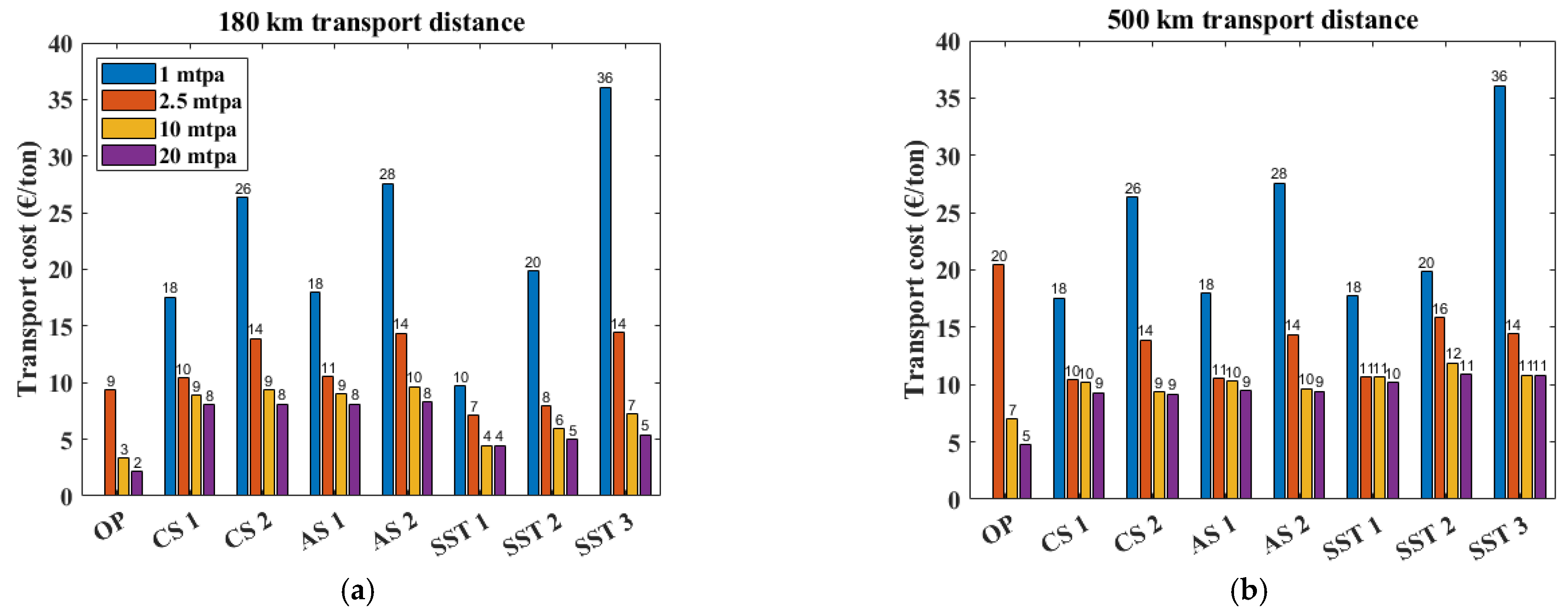
4.2.2. Short Distances (180 km)

The SST has the lowest cost for the smallest CO2 volumes of 1–2.5 mtpa. The main reason for the low cost is because this small volume can be served by 1–2 of the smallest SST, i.e., cargo volume of 10,569 m3, while the smallest crewed tanker ship is oversized. This results in a lower CAPEX and OPEX for the SST. The offshore pipeline is not considered in the 1 mtpa case.
The offshore pipeline has the lowest costs for the 10 and 20 mtpa cases. The offshore pipeline is well known to be the most cost-effective for large transportation volumes over short distances [40].

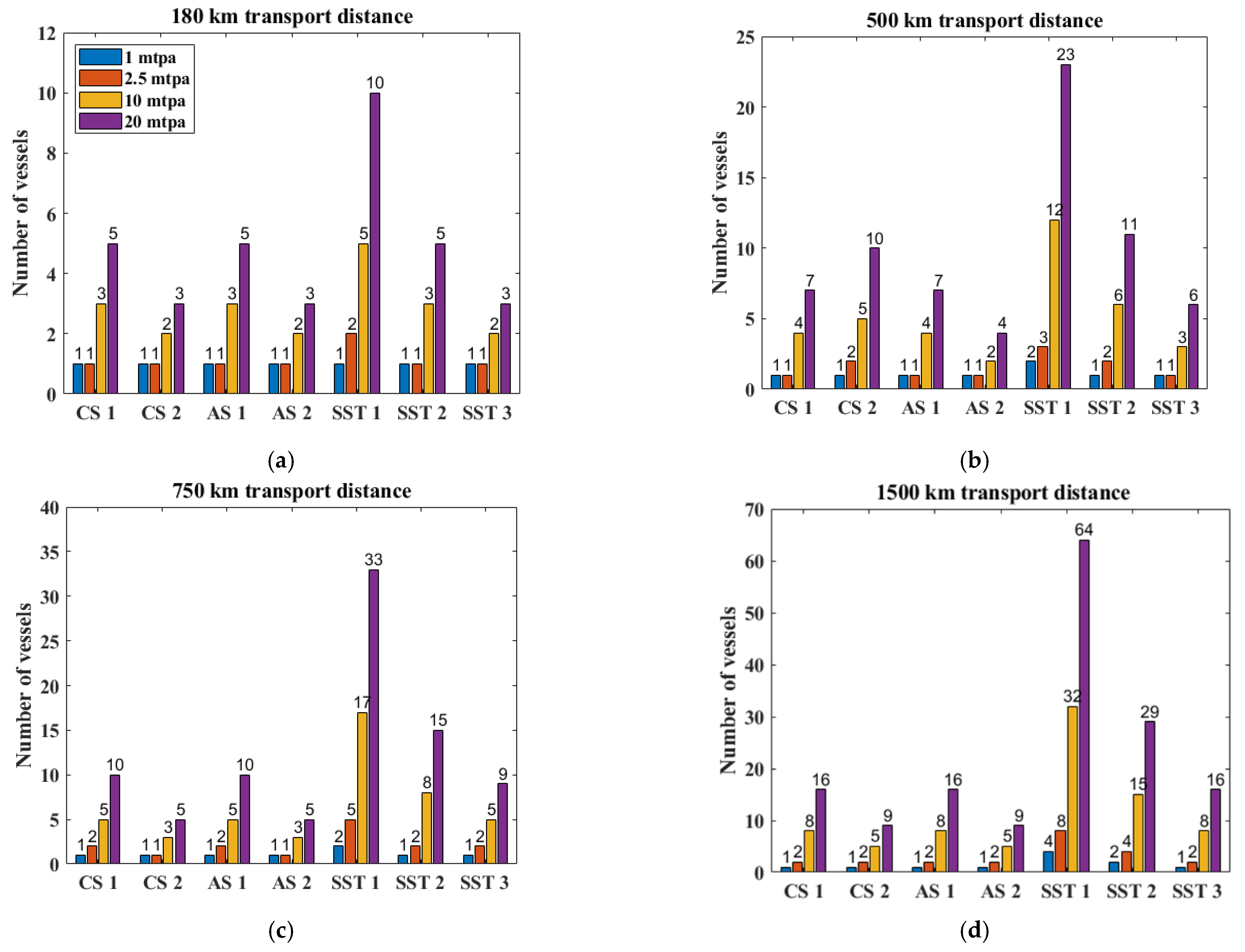
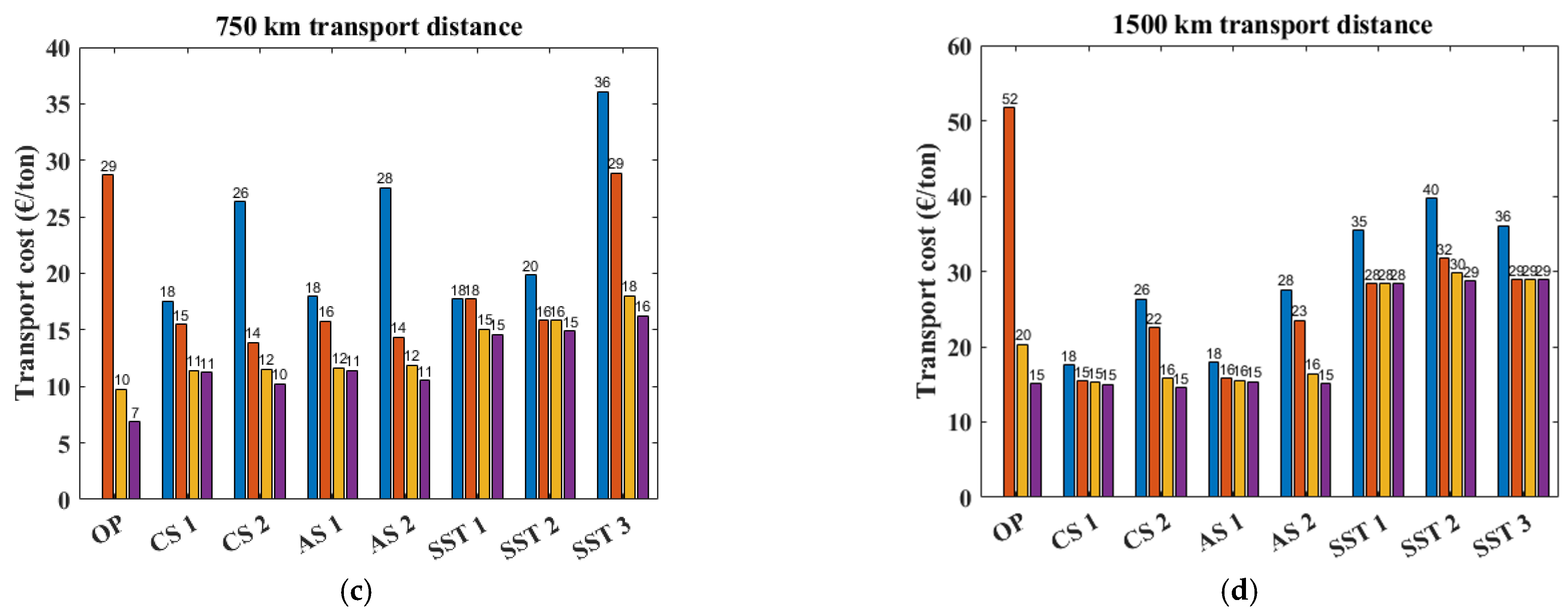
4.2.3. Intermediate and Long Distances (500–1500 km)

The SST has a low travelling speed and therefore requires more vessels to meet the larger CO2 volume requirements (>1 mtpa). This leads to a significantly higher CAPEX, and consequently a significantly higher cost per ton of CO2 compared to the crewed tanker ship. For example, for the 1500 km and 20 mtpa CO2 volume case, the SST requires 16–64 vessels while the crewed tanker ship only requires 9–16 vessels. The SST CAPEX is 5314–5461 m€ compared to 1563–1638 m€ for the crewed tanker CAPEX. The cost per ton of CO2 is 28–29 € compared to 15 €/ton of CO2, respectively. The SST is nevertheless competitive for the smallest CO2 volumes of 1–2.5 mtpa. It is expected that if the SST speed is adjusted to better fit the transportation distance and annual transportation capacity the cost can be optimized, and thus reduced. Although not considered in this paper, this is definitely of interest for future study.
For intermediate distances of 500–750 km and large CO2 volumes of 10–20 mtpa, the offshore pipeline has the lowest costs at 5–10 €/ton of CO2. It is well-known that offshore pipelines are the most cost-effective solution for large transport volumes over short and intermediate distances [40]. The crewed tanker ship, however, is not far behind at 9–11 €/ton of CO2.

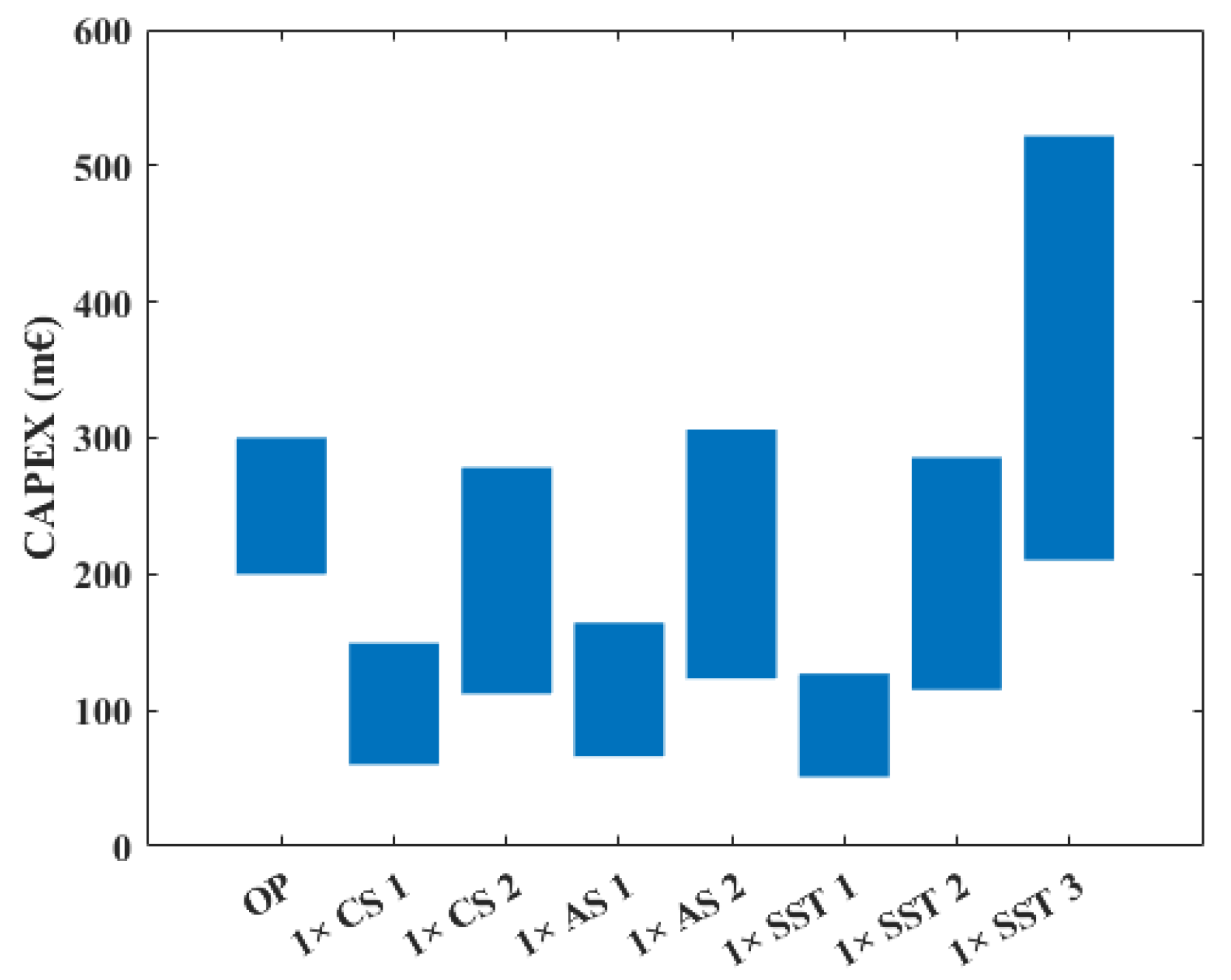
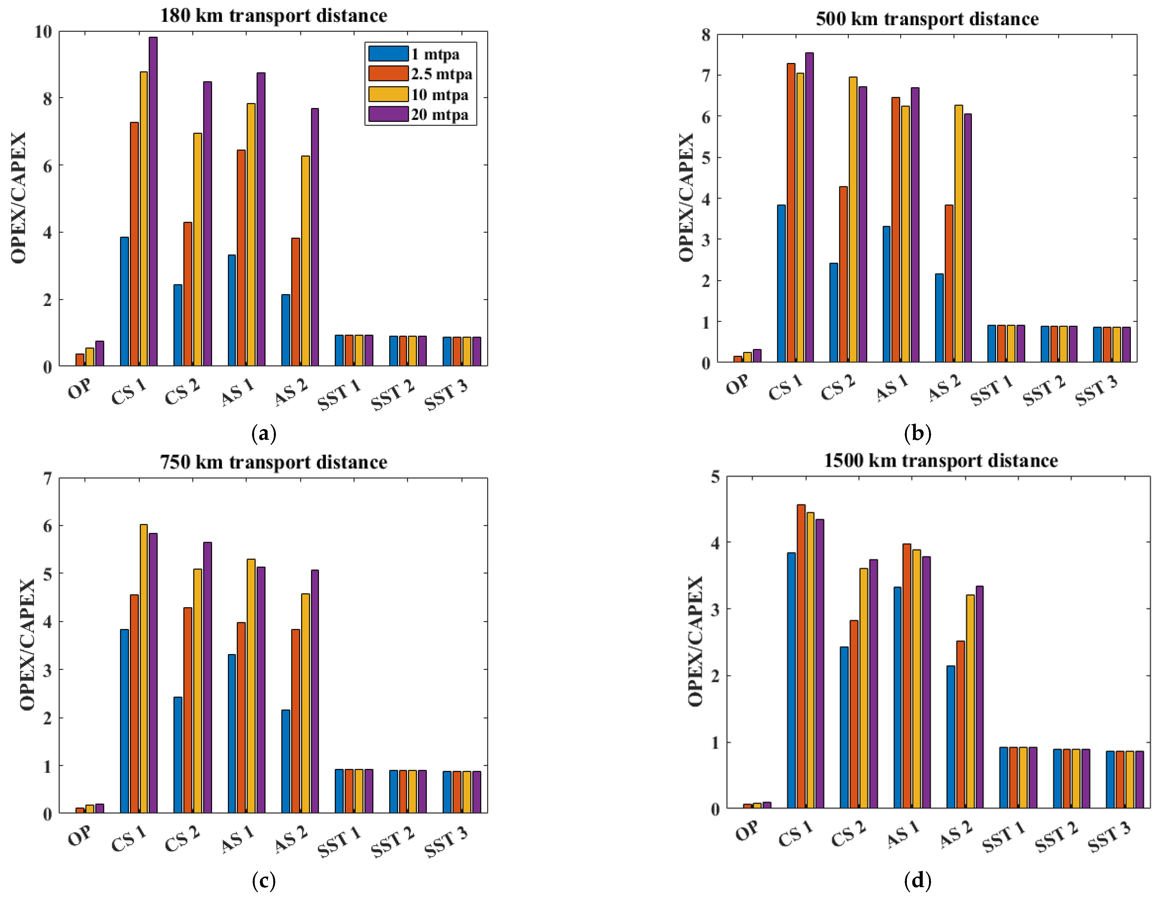
4.2.4. CAPEX and OPEX

To achieve better insight into the cost picture, the CAPEX and OPEX are studied in more detail in this section. The CAPEX for all transportation methods is presented in Figure 9. It is observed that the SST CAPEX increases more rapidly with size compared to the tanker ship. This reinforces the fact that the SST is not a cost-effective option when large transportation volumes are required. This higher cost is also reflected in the results presented in Figure 7 for the 10 and 20 mtpa CO2 volumes.
The main reason for the SST’s high CAPEX is its heavy structural weight. This is because the SST is designed based on DNVGL-RU-NAVAL-Pt4Ch1 [16], which is primarily catered towards military submarine design. It is expected that a dedicated structural design code that is optimized for the SST would significantly reduce the safety factors required. This could reduce the structural weight and corresponding CAPEX. For example, the probabilistic design method presented in Arbocz and Stam [41] applied to thin shell structures under axial loading can reduce the safety factor as much as twofold. This highlights the enormous potential for significant structural weight reductions in the future.
The OPEX-to-CAPEX ratios are presented in Figure 10. From the figure, it can be seen that the cost for tanker ships is OPEX-dominated; OPEX/CAPEX is 3.84–9.82. In contrast, the cost for offshore pipelines is CAPEX-dominated; OPEX/CAPEX is 0.06–0.75. For the SST, the OPEX is fairly similar to the CAPEX; OPEX/CAPEX is 0.87–0.92.

4.2.5. Crewed vs. Autonomous Tanker Ship

The crewed tanker ship is found to be slightly cheaper (up to 8%) compared to the autonomous tanker ship. This contrasts with the results presented in MUNIN D9.3 report [22], where the autonomous version of a specific bulker ship is up to 8.6% cheaper than its crewed counterpart. The first reason is due to the low CAPEX for the bulker ship used in MUNIN D9.3 report [22]. The MUNIN ship’s CAPEX is 34 m€. The tanker ships considered in this paper are CO2 carriers that carry expensive equipment and have a CAPEX of 60–278 m€. The second reason is the use of the assumption that OPEX is defined to be 2% CAPEX. The combination of these two reasons leads to a higher resulting OPEX (17.03–21.39 m€/a) in the tanker ships considered in this paper versus 4.33 m€/a for the MUNIN bulker ship. This higher OPEX dwarfs the crew operating costs of 0.64 m€/a. Due to the lower CAPEX and correspondingly lower OPEX, the crewed tanker ship becomes slightly cheaper than the autonomous tanker ship. Nevertheless, the costs per CO2 ton reported for the crewed and autonomous ships are similar and within the uncertainty bands that would be expected in a cost analysis [42].

5. Conclusions

In this paper, a technical–economic analysis of the SST is performed. The analysis is performed in two steps. First, the SST’s technical feasibility is evaluated by investigating designs with lower and higher capacities. The purpose is to observe the appearance of technical limits (if present) when the SST is scaled down or up in size. Second, an economic analysis is performed using the well-reviewed cost models from the publicly available ZEP [21] and MUNIN D9.3 [22] reports. The scenarios considered are CO2 transport volumes of 1 to 20 mtpa with transport distances of 180 to 1 500 km in which the cost per ton of CO2 is compared between offshore pipelines, crewed/autonomous tanker ships, and SST. The results show that SSTs with cargo capacities of 10,569 m3, 23,239 m3, and 40,730 m3 are technically feasible. Furthermore, SSTs are competitive for short and intermediate distances of 180–750 km and for smaller CO2 volumes of 1–2.5 mtpa. In addition, it is found that the SST has a higher CAPEX and lower OPEX compared with tanker ships. This is mainly due to the SST having a slow travelling speed, using electricity for propulsion, and carrying CO2 in the saturated state, i.e., there is no liquefaction cost. Finally, it must be mentioned that the SST designs analysed here use DNVGL-RU-NAVAL-Pt4Ch1 [16], which is primarily catered towards military submarine design. It is expected that a dedicated structural design code that is optimized for SST design could substantially reduce their structural weight and corresponding CAPEX.

Author Contributions

Conceptualization, Y.X. and Y.M.; methodology, Y.X. and Y.M.; software, T.A.D.S. and Y.M.; validation, T.A.D.S. and Y.M.; formal analysis, Y.X., T.A.D.S. and Y.M.; investigation, Y.X., T.A.D.S. and Y.M.; resources, Y.X.; data curation, T.A.D.S. and Y.M.; writing—original draft preparation, Y.X.; writing—review and editing, Y.X. and Y.M.; visualization, T.A.D.S. and Y.M.; supervision, Y.X. and Y.M.; project administration, Y.X.; funding acquisition, Y.X. All authors have read and agreed to the published version of the manuscript.

Funding

This research received no external funding.

Institutional Review Board Statement

Not applicable.

Informed Consent Statement

Not applicable.

Data Availability Statement

Not applicable.

Conflicts of Interest

The authors declare no conflict of interest.

Appendix A

External hull design calculations for SST 1: Subsea shuttle tanker (Cargo 10,569 m3)
The design calculation method in DNVGL-RU-NAVAL-Pt4Ch1 [26], Appendix A, Section 6 is applied to determine the SST’s external hull properties. The calculation inputs and processes are provided in Table A1. The symbols and equation numbers are aligned with the notation used in the DNVGL guideline. Table A2, Table A3, Table A4 and Table A5 present the stresses in the free flooding compartments and flooded mid-body external hulls. The external hulls in the free flooding compartments are subjected to hydrostatic pressures and are checked against permissible stresses at the nominal diving depth, test diving depth, and collapse depth in accordance with Chapter 4 in DNVGL-RU-NAVAL-Pt4Ch1 [26]. The permissible values are listed in Table A6.
Table A1. External hull calculation for SST 1: Subsea shuttle tanker (Cargo 10 569 m3).
Parameter SymbolUnitsFree Flooding CompartmentFlooded
COMPARTMENT
Equation Number in DNVGL RU P4Cl
Appendix A
Design Pressure Type Nominal Diving DepthTest Diving DepthCollapse DepthCollapse
Design pressurep(bar)710.5197User input
Hull thicknesss(m)0.0290.0290.0290.019User input
Hull radiusRm(m)6.56.56.56.5User input
Frame web heighthw(m)0.30.30.30.3User input
Frame web thicknesssw(m)0.030.030.030.03User input
Flange widthbf(m)0.10.10.10.1User input
Flange thicknesssf(m)0.0330.0330.0330.033User input
Frame spacingLF(m)1111.5User input
Frame cross sectional areaAF(m)0.01230.0120.01230.0123User input
Inner radius to the flange of frameRf(m)6.1386.138 6.1386.138User input
Youngs modulusE(GPa)206206206206User input
Poisson Ratiov 0.30.30.30.3User input
Poisson ratio in elastic-plastic rangevp 0.440.440.440.44(A48)
Frame distance without thicknessL(m)0.970.970.9 0.97(A9)
Effective lengthLeff(m)0.650.650.650.625(A10)
Effective areaAeff(m2)0.01260.01260.01260.012(A11)
The radial displacement in the middle between the frameswM(m)−0.003−0.007−0.0125−0.0076(A15)
The radial displacement at the frameswF(m)−0.0041−0.008−0.0148−0.0012(A16)
The reference stress is the circumferential stress in the unstiffened cylindrical pressure hullσo(MPa)156.9235.3425.9239.5(A13)
The equivalent stresses are composed of the single stresses in longitudinal and circumferential direction at the middle between framesσmv,m(MPa)104.77157.26287.3 240 (A14)
The equivalent stresses are composed of the single stresses in longitudinal and circumferential direction at the framesσmv,f(MPa)133.4184.43326.9104.75(A14)
Average membrane stress in longitudinal directionσmx(MPa)78.5117.67212.9119.7(A17)
Membrane stress in circumferential direction in the middle between the framesσmϕ,M(MPa)118.98178.6326.8276.3(A18)
Membrane stress in circumferential direction at the framesσmϕ,F(MPa)154212.55376.474.7(A19)
Bending stresses in longitudinal direction in the middle between the framesσxϕ,M(MPa)63.9105.224071.2(A20)
Bending stresses in longitudinal direction at the framesσbx,F(MPa)541.695.98300(A21)
Bending stresses in circumferential direction in the middle between the framesσbϕ,M(MPa)19.231.57221.4(A22)
Bending stresses in circumferential direction at the framesσbϕ,F(MPa)1.512.528.890(A23)
Tangential moduleEt(GPa)206206206206(A38)
Secant moduleEs(GPa)204204204204(A39)
Elastic buckling pressurepelcr(bar)56565664(A28)
Theoretical elastic-plastic buckling pressurepicr(bar)56565664(A29)
Reduction factorR 0.750.750.750.75(A43)
Elastic-plastic buckling pressurepcr(bar)42424248(A45)
Table A2. Stresses in the free flooding compartment (normal diving depth) for SST 1: Subsea shuttle tanker (Cargo 10,569 m3).
Type of StressesAt the FrameIn the Middle of the Field
Circum-FerentialEquivalentAxialCircum-FerentialEquivalentAxial
Membrane stress154.00 MPa-78.50 MPa118.98 MPa-78.50 MPa
Membrane equivalent stress-133.40 MPa--104.77 MPa-
Bending stresses1.50 MPa-5.00 MPa19.20 MPa-63.90 MPa
Normal stress outside155.50 MPa-83.50 MPa138.18 MPa-142.40 MPa
Equivalent normal stress outside-134.50 MPa--140.30 MPa-
Normal stress inside152.50 MPa-−5.00 MPa−19.20 MPa-14.60 MPa
Equivalent normal stress inside-134.50 MPa--140.30 MPa-
Table A3. Stresses in the free flooding compartment (test diving depth) for SST 1: Subsea shuttle tanker (Cargo 10,569 m3).
Type of StressesAt the FrameIn the Middle of the Field
Circum-FerentialEquivalentAxialCircum-FerentialEquivalentAxial
Membrane stress212.55 MPa-117.67 MPa178.60 MPa-117.67 MPa
Membrane equivalent stress-184.43 MPa--157.26 MPa-
Bending stresses12.50 MPa-41.60 MPa31.50 MPa-105.20 MPa
Normal stress outside225.05 MPa-159.27 MPa210.10 MPa-222.87 MPa
Equivalent normal stress outside-200.40 MPa--216.77 MPa-
Normal stress inside200.05 MPa-−41.60 MPa−31.50 MPa-12.47 MPa
Equivalent normal stress inside-200.40 MPa--216.77 MPa-
Table A4. Stresses in the free flooding compartment (collapse diving depth) for SST 1: Subsea shuttle tanker (Cargo 10 569 m3).
Type of StressesAt the FrameIn the Middle of the Field
Circum-FerentialEquivalentAxialCircum-FerentialEquivalentAxial
Membrane stress376.40 MPa-212.90 MPa326.80 MPa-212.90 MPa
Membrane equivalent stress-326.90 MPa--287.33 MPa-
Bending stresses28.80 MPa-95.98 MPa72.00 MPa-240.00 MPa
Normal stress outside405.20 MPa-308.88 MPa398.80 MPa-452.90 MPa
Equivalent normal stress outside-366.65 MPa--428.50 MPa-
Normal stress inside347.60 MPa-−95.98 MPa−72.00 MPa-−27.10 MPa
Equivalent normal stress inside-366.65 MPa--428.50 MPa-
Table A5. Stresses in the flooded compartment (collapse diving depth) for SST 1: Subsea shuttle tanker (Cargo 10,569 m3).
Type of StressesAt the FrameIn the Middle of the Field
Circum-FerentialEquivalentAxialCircum-FerentialEquivalentAxial
Membrane stress74.70 MPa-119.70 MPa276.30 MPa-119.70 MPa
Membrane equivalent stress-104.75 MPa--240.00 MPa-
Bending stresses90.00 MPa-300.00 MPa21.40 MPa-71.20 MPa
Normal stress outside164.70 MPa-419.70 MPa297.70 MPa-190.90 MPa
Equivalent normal stress outside-366.40 MPa--261.20 MPa-
Normal stress inside−15.30 MPa-−300.00 MPa−21.40 MPa-48.50 MPa
Equivalent normal stress inside-366.40 MPa--261.20 MPa-
Table A6. Equivalent stresses and permissible stresses for external hull for SST 1: Subsea shuttle tanker (Cargo 10,569 m3).
CaseDepthMaximum Equivalent StressPermissible Stress
(Ref. Sec. 4.3 in DNVGL RU P4C1)
Criterion Fulfilled?
Nominal diving depth70 m155.50 MPa203 MPaYes
Test diving depth105 m225.05 MPa418 MPaYes
Collapse depth190 m452.90 MPa460 MPaYes
Flooded Compartment-419.70 MPa460 MPaYes
Internal tank design calculations for half-scaled SST (10,569 m3)
The internal tanks in the SST are designed in accordance with Chapter 4 in ASME BPVC Section VIII, Division 2 [27]. In the SST, main cargo tanks, auxiliary cargo tanks, compensation tanks, and trim tanks are designed to take burst pressure. The buoyancy tubes are designed against collapse pressure.
For burst pressure design of all tanks except the buoyancy tubes, Chapters 4.3.3 and 4.3.5 in ASME VIII-2 [27] are used to determine the hull thicknesses for the cylindrical shells and hemisphere heads, respectively. The minimum required thickness of a cylindrical hull under internal pressure is expressed as:
t s h e l l = D t 2 ( e x p [ p i S a × E w ] 1 )
where tshell is the hull thickness, Dt is the tank diameter, and Sa is the allowable stress of material. Ew is the weld joint efficiency and is set to be 1.0 for circumferential joints and longitudinal joints on a shell (Ref. Table 7.2 in ASME VIII-2 [27]). pi is the design pressure and is defined to be 55 bar for the cargo tanks, trim and composition tanks.
Similarly, the minimum required thickness of a hemisphere heads under internal pressure is expressed as:
t s h e l l = D t 2 ( e x p [ 0.5 × p i S a × E w ] 1 )
For the collapse pressure design of the buoyancy tubes, Chapter 4.4.5 in ASME VIII-2 [27] is used. The step-by-step calculation process is presented in Table A7.
Table A7. Buoyancy tube calculation for SST 1: Subsea shuttle tanker (Cargo 10,569 m3).
ParameterSymbol in ASME BPVC Sec. VIII Div. 2ValueEquation Number in ASME BPVC Sec. VIII Div 2.
Thicknesst0.01 mUser input
Outer diameterDo0.9 mUser input
Unsupported lengthL3 mUser input
Young’s modulusEy200 GPaUser input
Minimum yield strengthSy414 MPaUser input
Design factorFS2(4.4.1)
Predicted elastic buckling stressFhe71 MPa(4.4.19)
FactorMx45(4.4.20)
FactorCh0.02(4.4.22)
Predicted buckling stressFic71 MPa(4.4.27)
Allowable external pressurePa8 bar(4.4.28)

Appendix B

The calculations for the economic analysis for the 180 km and 2.5 mtpa case are presented in this appendix. The following notations are used OP: Offshore pipeline; CS 1: Crewed ship (Cargo 22,000 m3); CS 2: Crewed ship (Cargo 41,000 m3); AS 1: Autonomous ship (Cargo 22,000 m3); AS 2: Autonomous ship (Cargo 41,000 m3); SST 1: Subsea shuttle tanker (Cargo 10,569 m3); SST 2: Subsea shuttle tanker (Cargo 23,239 m3); SST 3: Subsea shuttle tanker (Cargo 40,730 m3).
CAPEX—Offshore pipelines
The CAPEX values for the offshore pipelines are taken from Annex 3 in the ZEP report [21]. The contingency is 20%.
CAPEX—Tanker ships and SSTs
Equation (A3) is used to calculate the CAPEX calculations of the tanker ships and SSTs. The corresponding CAPEXs are presented in Table A8.
CAPEX = Steel   price   × Vessel   structure   volume
The annuity is calculated using Equation (A4). The lifetime is 40 years and the discount rate is 8%.
Annuity = CAPEX · discount   rate 1 ( 1 + discount   rate ) . lifetime
Example CAPEX calculations
Table A8. CAPEX calculation for average values (180 km and 2.5 mpta).
OPCS 1AS 1SST 1Units
Price per ton of vessel steelN.A.18,896.0€/tonne
Structural volume517051704394tonne
Autonomous ship factorN.A.110%N.A.
CAPEX250.397.7107.583.0m€
Annuity20.998.199.016.96m€
OPEX—Offshore pipelines
The OPEX values are taken from the ZEP report [21] and are 2.35 m€/a, 4.76 m€/a, and 7.9 m€/a for 2.5 mtpa, 10 mtpa, and 20 mpta CO2 volumes, respectively.
OPEX—Tanker ships and SSTs
The OPEX of crewed tanker ship, autonomous tanker ship, and SST is calculated sing Equations (A5), (A6) and (A7), respectively.
OPEX CS = Maintenance + Crew + Fuel + Liquefaction
OPEX AS = Maintenance + Fuel + Liquefaction
OPEX SST = Maintenance + Electricity
Example OPEX calculations
The OPEX calculations for the average values for the offshore pipelines and the smallest size of the crewed ship, autonomous ship and SST are presented in Table A9.
Table A9. OPEX calculation for average values.
OPCS 1AS 1SST 1Units
Vessel maintenanceN.A.2%2%2%of CAPEX
CAPEX97.7107.583.0m€
Vessel maintenance cost1.952.151.66m€/year
Crew cost0.64N.A.N.A.m€/year
Fuel consumptions 9.139.13tonne/day
Fuel price573.33573.33€/tonne
Fuel cost1.911.91m€/year
Liquefaction cost for 2.5 mtpa13.2813.28m€/year
Electricity consumptionsN.A.N.A.6001kWh/day
Electricity price0.11€/kWh
Electricity cost0.24m€/year
OPEX2.3517.7817.331.90m€/year
Number of ships/SSTs required
The number of ships or SSTs required are calculated following Equation (A8).
N = roundup ( V CO 2 V v   ρ CO 2 365 2 L t U v + 2 T L )
where N is the number of ships, V C O 2 is the total CO2 volume per annum, V v is the total cargo volume for one vessel, ρ C O 2 is the density of carbon dioxide, L t is the transport distance, U v is the vessel speed, and T L is the loading/offloading time.
For example, the calculations to obtain the number of SST 1: Subsea shuttle tanker (Cargo 10,569 m3) required for 180 km and 2.5 mtpa are presented in Table A10.
Table A10. Number of ships required—SST 1: Subsea shuttle tanker (Cargo 10,569 m3).
ParametersValueUnits
Total CO2 volume2.50Mtpa
Cargo volume—SST 110 569m3
CO2 density0.94ton / m3
Transport distance180Km
Speed—SST 16Knots
Loading/offloading time—SST 14Hours
Number of ships required2
Cost of CO2 per tonne
The cost of CO2 per tonne is calculated using Equation (A9).
CO 2   cost = Annuity + OPEX Total   CO 2   per   annual
The cost of CO2 per tonne calculations for the 180 km and 2.5 mtpa case are presented in Table A11.
Table A11. Cost of CO2 per tonne—180 km and 2.5 mtpa.
OPCS 1AS 1SST 1
Annuity20.99 m€8.19 m€9.01 m€13.93 m€
OPEX2.35 m€17.78 m€17.33 m€3.80 m€
Total CO2 per annual2.5
CO2 per tonne9.33€10.39€10.54€7.09€

Notes

1
To prevent confusion with Subsea Shuttle Tanker (SST), shuttle tanker ships will be refered as tanker ships in the remainder of the text.
2
The maximum range is 400 km for the baseline SST. This range is extended by fitting additional batteries for longer ranges. See also Section 2.6.

References

  1. Fullenbaum, R.; Fallon, J.; Flanagan, B. Oil & Natural Gas Transportation & Storage Infrastructure: Status, Trends, & Economic Benefits; Technical report; IHS Global Inc.: Washington, DC, USA, 2013. [Google Scholar]
  2. Palmer, A.; King, R. Subsea Pipeline Engineering, 2nd ed.; PennWell Corp.: Tulsa, OK, USA, 2008. [Google Scholar]
  3. Vestereng, C. Shuttle Tankers in Brazil. Available online: https://www.dnv.com/expert-story/maritime-impact/shuttle-tankers-Brazil.html (accessed on 1 August 2021).
  4. Wilson, J. Shuttle tankers vs pipelines in the GOM frontier. World Oil 2008, 4, 149–151. [Google Scholar]
  5. Equinor Energy AS. RD662093 Subsea Shuttle System, 2019.
  6. Ellingsen, K.E.; Ravndal, O.; Reinas, R.; Hansen, J.H.; Marra, F.; Myhre, E.; Dupuy, P.M.; Sveberg, K. RD677082 Subsea Shuttle System, 2020.
  7. Xing, Y.; Ong, M.C.; Hemmingsen, T.; Ellingsen, K.E.; Reinas, L. Design considerations of a subsea shuttle tanker system for liquid carbon dioxide transportation. J. Offshore Mech. Arct. Eng. 2021, 143, 045001. [Google Scholar] [CrossRef]
  8. Ma, Y.; Xing, Y.; Ong, M.C.; Hemmingsen, T. Baseline design of a subsea shuttle tanker system for liquid carbon dioxide transportation. J. Ocean Eng. 2021, 240, 109891. [Google Scholar] [CrossRef]
  9. Jacobsen, L.R. Subsea Transport of Arctic Oil—A Technical and Economic Evaluation. In Proceedings of the Offshore Technology Conference, Houston, TX, USA, 2 May 1971. [Google Scholar]
  10. Taylor, P.; Montgomery, J. Arctic Submarine Tanker System. In Proceedings of the Offshore Technology Conference, Houston, TX, USA, 2 May 1977. [Google Scholar]
  11. Jacobsen, L.; Lawrence, K.; Hall, K.; Canning, P.; Gardner, E. Transportation of LNG from the Arctic by commercial submarine. Mar. Technol. SNAME News 1983, 20, 377–384. [Google Scholar] [CrossRef]
  12. Xing, Y. A Conceptual Large Autonomous Subsea Freight-Glider for Liquid CO2 Transportation. In Proceedings of the International Conference on Offshore Mechanics and Arctic Engineering, Online Conference, 21–30 June 2021. [Google Scholar]
  13. Norwegian Petroleum Directorate (NPD). Carbon Capture and Storage. Available online: http://www.norskpetroleum.no/en/environment-and-technology/carbon-capture-and-storage (accessed on 1 August 2021).
  14. Equinor ASA. Northern Lights CC. Available online: https://www.equinor.com/en/what-we-do/northern-lights.html (accessed on 1 August 2021).
  15. Ma, Y.; Sui, D.; Xing, Y.; Ong, M.C.; Hemmingsen, T.H. Depth control modelling and analysis of a subsea shuttle tanker. In Proceedings of the International Conference on Ocean, Offshore and Artic Engineering, Online Conference, 21–30 July 2021. [Google Scholar]
  16. Ma, Y.; Xing, Y.; Hemmingsen, T.H. An evaluation of key challenges of CO2 transportation with a novel Subsea Shuttle Tanker. In Proceedings of the Third Conference of Computational Methods in Offshore Technology, Stavanger, Norway, 25–26 November 2021. [Google Scholar]
  17. Ma, Y.; Xing, Y.; Silva, M.S.D.; Sui, D. Modelling of a subsea shuttle tanker hovering in ocean current, under review. In Proceedings of the International Conference on Ocean, Offshore and Arctic Engineering, Hamburg, Germany, 5–10 June 2022. [Google Scholar]
  18. Taylor, P. Energy Technology Perspectives 2010: Scenarios and Strategies to 2050; OECD Publishing: Paris, France, 2010. [Google Scholar]
  19. Papanikolaou, A. Ship Design: Methodologies of Preliminary Design. Springer: Manhattan, NY, USA, 2014. [Google Scholar]
  20. Carbon Capture and Storage Association (CCSA). What Is CCS. Available online: http://www.ccsassociation.org/what-is-ccs/ (accessed on 30 September 2020).
  21. Zero Emissions Platform (ZEP). The Cost of CO2 Transport: Post-Demonstration CCS in the EU; Technical Report; Zero Emissions Platform: Brussels, Belgium, 2011. [Google Scholar]
  22. Kretschmann, L.; Rødseth, Ø.J.; Fuller, B.S.; Noble, H.; Horahan, J.; McDowell, H. MUNIN. Deliverable 9.3: Quatitative Assessment; MUNIN Report: 2015. Available online: http://www.unmanned-ship.org/munin/wp-content/uploads/2015/10/MUNIN-D9-3-Quantitative-assessment-CML-final.pdf (accessed on 1 October 2021).
  23. Stanković, J.J.; Marjanović, I.; Papathanasiou, J.; Drezgić, S. Social, Economic and Environmental Sustainability of Port Regions: MCDM Approach in Composite Index Creation. J. Mar. Sci. Eng. 2021, 9, 74. [Google Scholar] [CrossRef]
  24. Sifakis, N.; Tsoutsos, T. Planning zero-emissions ports through the nearly zero energy port concept. J. Clean. Prod. 2021, 286, 125448. [Google Scholar] [CrossRef]
  25. Wang, Z.; Wu, X.; Guo, J.; Wei, G.; Dooling, T.A. Efficiency evaluation and PM emission reallocation of China ports based on improved DEA models. Transp. Res. Part D Transp. Environ. 2020, 82, 102317. [Google Scholar] [CrossRef]
  26. DNV-GL Rules for Classification, Naval Vessels, Part 4 Sub-Surface Ships. Available online: https://rules.dnv.com/docs/pdf/DNV/RU-NAVAL/2018-01/DNVGL-RU-NAVAL-Pt4Ch1.pdf (accessed on 1 August 2021).
  27. ASME. Boiler and Pressure Vessel Code, Section VIII, Division 2; The American Society of Mechanical Engineers: New York, NY, USA, 2015. [Google Scholar]
  28. National Centers for Environmental Information (NCEI). Greenland, Iceland and Norwegian Seas Regional Climatology. Available online: https://www.ncei.noaa.gov/products/greenland-iceland-and-norwegian-seas-regional-climatology (accessed on 30 September 2020).
  29. Mariano, A.; Ryan, E.; Perkins, B.; Smithers, S. The Mariano Global Surface Velocity Analysis 1.0; Technical report No. CG-D-34-95; United States Coast Guard Research and Development Centre: New London, CA, USA, 1995. [Google Scholar]
  30. Ersdal, G. An Overview of Ocean Currents with Emphasis on Currents on the Norwegian Continental Shelf; Technical Report; Norwegian Petroleum Directorate: Stavanger, Norway, 2001. [Google Scholar]
  31. Sætre, R. The Norwegian Coastal Current: Oceanography and Climate; Fagbokforlaget: Bergen, Norway, 2007. [Google Scholar]
  32. ITTC Resistance Committee 26th. Recommended Procedures and Guidelines: Resistance Test; International Towing Tank Committee (ITTC): Zürich, Switzerland, 2011. [Google Scholar]
  33. Hoerner, S.F. Fluid-Dynamic Drag: Practical Information on Aerodynamic Drag and Hydrodynamic Resistance; Hoerner Fluid Dynamics: Bakersfield, CA, USA, 1965. [Google Scholar]
  34. Barnitsas, M.M.; Ray, D.; Kinley, P. KT, KQ and Efficiency Curves for the Wageningen B-Series Propellers; Technical Report; University of Michigan: Ann Arbor, MI, USA, 1981. [Google Scholar]
  35. Renilson, M. Submarine Hydrodynamics; Springer: Cham, Switzerland, 2015. [Google Scholar]
  36. WSD50 30K 30,000 M3 LNG Carrier Data Sheet. Available online: https://cdn.wartsila.com/docs/default-source/product-files/sd/merchant/lng/wsd50-30k-lng-carrier-ship-design-o-data-sheet.pdf?sfvrsn=e8b38445_8 (accessed on 1 August 2021).
  37. Kretschmann, L.; Burmeister, H.C.; Jahn, C. Analyzing the economic benefit of unmanned autonomous ships: An exploratory cost-comparison between an autonomous and a conventional bulk carrier. Res. Transp. Bus. Manag. 2017, 25, 76–86. [Google Scholar] [CrossRef]
  38. Elsey, J. How to Define & Measure Centrifugal Pump Efficiency: Part 1. Available online: https://www.pumpsandsystems.com/how-define-measure-centrifugal-pump-efficiency-part-1#:~:text=Centrifugal%20pumps%20can%20approach%2094,will%20vary%20by%20plant%20type (accessed on 21 September 2021).
  39. Hall, S. Rules of Thumb for Chemical Engineers; Butterworth-Heinemann: Oxford, UK, 2017. [Google Scholar]
  40. Odland, J. Offshore Field Development; Course Compendium, University of Stavanger: Stavanger, Norway, 2018. [Google Scholar]
  41. Arbocz, J.; Stam, A.R. A Probabilistic Approach to Design Shell Structures, Buckling of Thin Metal Shells; Taylor & Francis: London, UK, 2004. [Google Scholar]
  42. Stephenson, L. Cost Engineers’ Notebook, 2nd ed.; AACE International: Morgantown, WV, USA, 2016. [Google Scholar]
Figure 1. Illustration of the Subsea Shuttle Tanker [8].
Jmse 10 00020 g001
Figure 2. CCS storage sites in the Norwegian sector [8].
Jmse 10 00020 g002
Figure 3. Offshore transportation methods for CCS.
Jmse 10 00020 g003
Figure 4. Design flow chart used in SST technical design.
Jmse 10 00020 g004
Figure 5. SST general arrangement. A, B, C, and D are the cut-through sections.
Jmse 10 00020 g005
Figure 6. Recalculation crewed ship CAPEX in comparison with ZEP results [21].
Jmse 10 00020 g006
Figure 7. Mean cost per ton of CO2 results on different source volumes and transport distances: (a) 180 km; (b) 500 km; (c) 750 km; (d) 1500 km. OP: Offshore pipeline; CS 1: Crewed ship (Cargo 22,000 m3); CS 2: Crewed ship (Cargo 41,000 m3); AS 1: Autonomous ship (Cargo 22,000 m3); AS 2: Autonomous ship (Cargo 41,000 m3); SST 1: Subsea shuttle tanker (Cargo 10,569 m3); SST 2: Subsea shuttle tanker (Cargo 23,239 m3); SST 3: Subsea shuttle tanker (Cargo 40,730 m3).
Jmse 10 00020 g007aJmse 10 00020 g007b
Figure 8. Number of vessels required on different source volumes and transport distances: (a) 180 km; (b) 500 km; (c) 750 km; (d) 1500 km.
Jmse 10 00020 g008
Figure 9. CAPEX estimations.
Jmse 10 00020 g009
Figure 10. CAPEX and OPEX ratio on different source volumes and transport distances: (a) 180 km; (b) 500 km; (c) 750 km; (d) 1500 km.
Jmse 10 00020 g010
Table 1. Baseline subsea shuttle tanker (SST) operating specifications.
ParameterValueUnit
Collapse depth190(m)
Operating depth (nominal diving depth)70(m)
Operating speed6(knots)
Maximum range2400(km)
Current speed1(m/s)
Cargo pressure35–55(bar)
Cargo temperature0–20(°C)
Table 2. SST structural design materials.
PropertiesMaterialYield StrengthTensile Strength
External hull—bow compartmentVL D47460 MPa550 MPa
External hull—mid-bodyVL D47460 MPa550 MPa
External hull—aft compartmentVL D47460 MPa550 MPa
Internal hull—main cargo tankSA-738 Grade B414 MPa586 MPa
Internal hull—auxiliary cargo tankSA-738 Grade B414 MPa586 MPa
Internal hull—comp. tankSA-738 Grade B414 MPa586 MPa
Internal hull—trim tankSA-738 Grade B414 MPa586 MPa
Internal hull—buoyancy tubeSA-738 Grade B414 MPa586 MPa
BulkheadVL D47460 MPa550 MPa
Table 4. Baseline design SST external hull properties.
ParameterUnitsSST 10,569 m3SST 23,239 m3SST 40,730 m3
Free flooding bow compartmentLength(m)18.5023.7528.85
Thickness(m)0.0290.0330.038
Steel Weight(ton)211.5389.5636.4
Design collapse pressure(bar)202020
Material VL D47VL D47VL D47
Flooded mid-bodyLength(m)75100122
Thickness(m)0.0190.0250.023
Steel Weight(ton)599.01380.01932.0
Design collapse pressure(bar)777
Material VL D47VL D47VL D47
Free flooding aft compartmentLength(m)3240.2549
Thickness(m)0.0290.0330.038
Steel Weight(ton)364.5663.71089.7
Design collapse pressure(bar)202020
Material VL D47VL D47VL D47
Table 5. SST internal tank properties.
ParameterUnitsSST 10,569 m3SST 23,239 m3SST 40,730 m3
Main Cargo Tank
(Total No. = 7)
Length(m)75100122
Diameter(m)4.005.006.20
Thickness(m)0.0460.0570.071
Hemisphere head wall thickness(m)0.0230.0290.036
Total volume(m3)648013,51525,346
Steel weight(ton)228447698936
Material SA-738 Grade BSA-738 Grade BSA-738 Grade B
Allowable burst pressure(bar)555555
Auxiliary Cargo Tank
(Total No. = 6)
Length(m)72.897.5118.8
Diameter(m)1.802.503.00
Thickness(m)0.0210.0290.034
Hemisphere head wall thickness(m)0.010.0150.017
Total volume(m3)1 1022 8474 996
Steel weight(ton)3901 0261 769
Material SA-738 Grade BSA-738 Grade BSA-738 Grade B
Allowable burst pressure(bar)555555
Compensation Tank
(Total No. = 2)
Length(m)111517.5
Diameter(m)5.508.0012.00
Thickness(m)0.010 0.0150.018
Total volume(m3)73316002864
Steel weight(ton)100200400
Material SA-738 Grade BSA-738 Grade BSA-738 Grade B
Allowable burst pressure(bar)888
Trim Tank
(Total No. = 2)
Length(m)3.556
Diameter(m)3.507.0014.00
Thickness(m)0.0100.0150.018
Total volume(m3)200400800
Steel weight(ton)3570140
Material SA-738 Grade BSA-738 Grade BSA-738 Grade B
Allowable burst pressure(bar)101010
Buoyancy Tube
(Total No. = 8)
Length(m)75100122
Diameter(m)0.901.251.60
Thickness(m)0.0100.0150.018
Total volume(m3)38210301954
Steel weight(ton)135368689
Material SA-738 Grade BSA-738 Grade BSA-738 Grade B
Allow. collapse pressure(bar)777
Table 6. Weight composition for individual SST design (CO2-filled condition).
ComponentWeight (Tons)
SST 10,569 m3SST 23,239 m3SST 40,730 m3
Payload712747.6%15,38145.8%28,52247.0%
Structure422028.2%930227.7%15,93726.2%
Machinery4493.0%10093.0%18223.0%
Mid-body seawater187712.5%490514.6%834113.7%
Compensation ballast7394.9%17795.3%38656.4%
Trim ballast1050.7%2350.7%4250.7%
Permanent ballast4493.0%10093.0%18223.0%
Sum14,966100%33,619100%60,734100%
Table 7. Hydrostatic stability check.
SST 10,569 m3
Submerged
(CO2 Filled)
Submerged
(SW Filled)
Surfaced
(CO2 Filled)
Surfaced
(SW Filled)
CoB (x,y,z)(−1.64, 0.00, 0.00)(−1.64, 0.00, 0.00)(−1.64, 0.00, 4.30)(−1.64, 0.00, 3.50)
CoG (x,y,z)(−2.31, 0.00, 1.13)(−2.01, 0.00, 1.48)(−2.32, 0.00, 1.51)(−2.63, 0.00, 2.20)
M (x,y,z)(0.00, 0.00, 0.00)(0.00, 0.00, 0.00)(0.00, 0.00, 0.00)(0.00, 0.00, 0.00)
GM1.131.481.512.20
BG1.131.482.791.30
ResultBG > 0.35 == OKBG > 0.35 == OKGM > 0.22 == OKGM > 0.22 == OK
SST 23,239 m3
Submerged
(CO2 Filled)
Submerged
(SW Filled)
Surfaced
(CO2 Filled)
Surfaced
(SW Filled)
CoB (x,y,z)(−1.44, 0.00, 0.00)(−1.44, 0.00, 0.00)(−1.44, 0.00, 4.30)(−1.44, 0.00, 3.50)
CoG (x,y,z)(−1.35, 0.00, 0.55)(−1.30, 0.00, 0.77)(−1.56, 0.00, 0.83)(−1.82, 0.00, 1.70)
M (x,y,z)(0.00, 0.00, 0.00)(0.00, 0.00, 0.00)(0.00, 0.00, 0.00)(0.00, 0.00, 0.00)
GM0.550.770.831.70
BG0.550.773.471.80
ResultBG > 0.35 == OKBG > 0.35 == OKGM > 0.22 == OKGM > 0.22 == OK
SST 40,730 m3
Submerged
(CO2 Filled)
Submerged
(SW Filled)
Surfaced
(CO2 Filled)
Surfaced
(SW Filled)
CoB (x,y,z)(−1.45, 0.00, 0.00)(−1.44, 0.00, 0.00)(−1.45, 0.00, 5.80)(−1.45, 0.00, 7.20)
CoG (x,y,z)(−1.04, 0.00, 0.43)(−0.94, 0.00, 0.53)(−1.18, 0.00, 0.58)(−1.39, 0.00, 1.66)
M (x,y,z)(0.00, 0.00, 0.00)(0.00, 0.00, 0.00)(0.00, 0.00, 0.00)(0.00, 0.00, 0.00)
GM0.430.530.581.66
BG0.430.535.225.54
ResultBG > 0.35 == OKBG > 0.35 == OKGM > 0.22 == OKGM > 0.22 == OK
Table 8. Main parameters of final derived SST designs.
Ship ParametersValue
Deadweight (ton)10,57223,72842,670
Deadweight (m3)10,56923,23940,730
Lightweight (ton)4394989118,064
Lightweight (m3)4032956018,522
Displacement (ton)14,96633,61960,734
Displacement (m3)14,60132,79959,252
Length (m)126164200
Beam (m)131721
Speed (knots)666
Travel distance design (km)400400400
Total power consumptions (kW)358,764620,249955,292
Power consumptions (kWh/day)600110,37515,477
Table 9. Cost models used from ZEP and MUNIN D9.3 reports.
Cost Model Used from ZEP [21]Cost Model Used from MUNIN D9.3 [22]
Project lifetime: 40 yearsDiscount rate 8%
Discount rate 8%Autonomous ship CAPEX Price
Ship transport speedFuel price
Transport distance casesShip fuel consumptions
Transport volume cases
Ship capacity
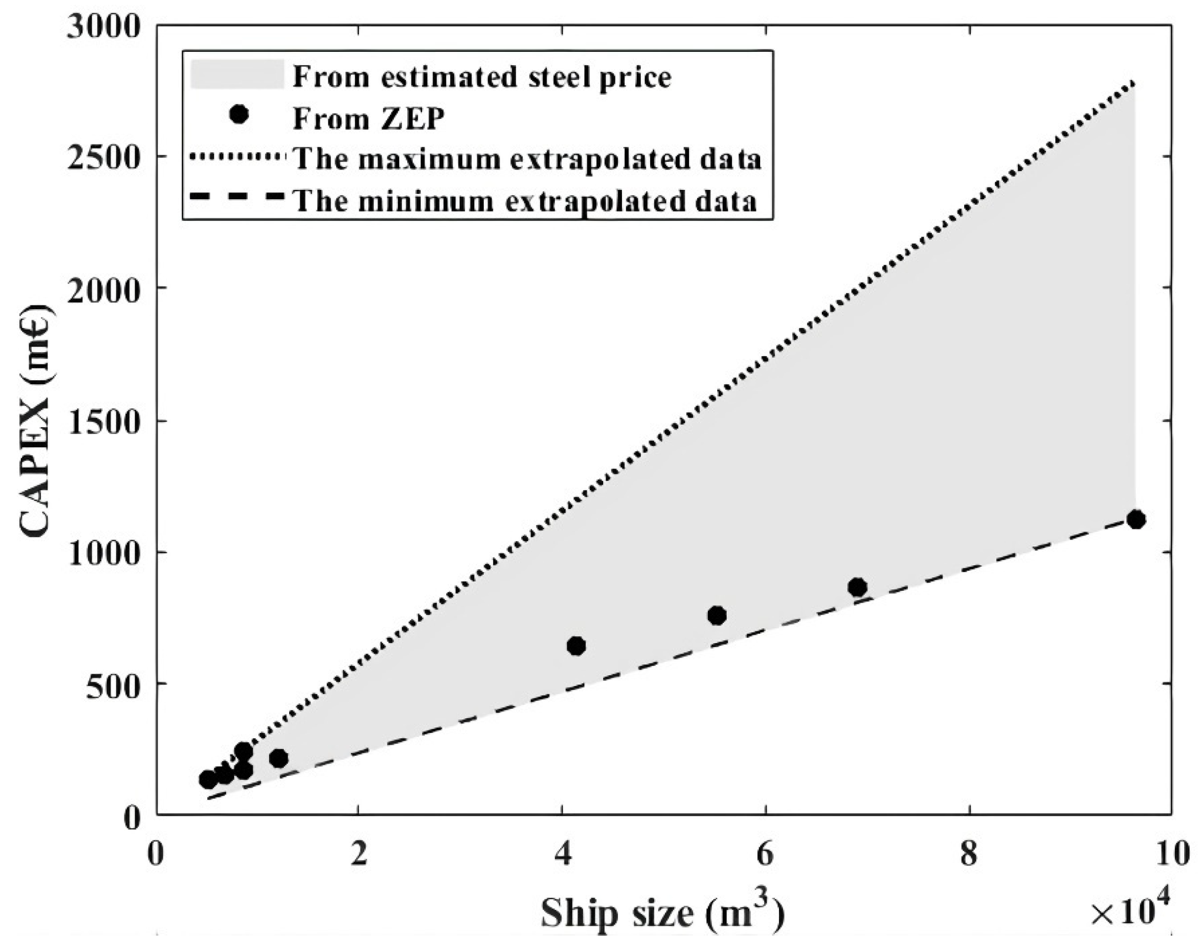
Ship CAPEX results (into steel price)
Ship operating expenditure (OPEX)
Offshore pipeline capital expenditure (CAPEX)
Offshore pipeline OPEX
Electricity price
Liquefaction price
Ship loading and offloading durations
Table 10. Offshore pipeline properties, data is analyzed and summarized from [21].
Offshore Pipelines—Properties
Pressures 250bar
Inlet pressure200bar
Outlet pressure60bar
Pipeline internal friction50μm
Pipeline materialCarbon steel
External coating3 mmPolypropylene (PP)
Concrete coating
(for pipeline above 16″)
70 mm/2600 kg/m3
Environmental factors assumptions
1.
The first 50 km is shallow with sand waves, and the remaining route is flat.
2.
100% burial requirement for pipeline dimensions equal to or below 16″.
3.
100% burial in sand wave area for all sizes
Installation method assumptionsTo give the necessary resistance to longitudinal crack propagation
Other assumptionsCO2 streams inside the pipeline are non-corrosive
Table 11. Offshore pipeline component pricing, data is analyzed and summarized from [21].
Offshore Pipelines—Component Pricing
Steel price for pipeline 16″160€/meter
Steel price for pipeline 40″700€/meter
External coating (anti-corrosion/weight) for pipeline 16″90€/meter
External coating (anti-corrosion/weight) for pipeline 40″200€/meter
Installation cost200–300€/meter
Trenching cost20–400€/meter
Contingency20%
Pipeline OPEX for 2.5 mtpa2.35m€/year
Pipeline OPEX for 10 mtpa4.76m€/year
Pipeline OPEX for 20 mtpa7.90m€/year
Table 12. Offshore pipeline annuities.
CO2 VolumeOffshore Pipeline Length
180 km500 km750 km1 500 km
2.5 mtpa20.99 m€48.69 m€69.41 m€126.96 m€
10 mtpa28.34 m€65.48 m€92.73 m€197.92 m€
20 mtpa35.54 m€86.83 m€130.16 m€293.60 m€
Table 13. Crewed/autonomous tanker ship properties, data is analyzed and summarized from [21].
Crewed/Autonomous Tanker Ship Properties
Speed14knots
Loading/offloading time12hours
Liquefaction 2.5 mtpa 5.31€/ton
Liquefaction 10 mtpa5.09€/ton
Liquefaction 20 mtpa 4.87€/ton
Fuel consumption, ship 22,000 m39.13ton/day
Fuel consumption, ship 45,100 m318.72ton/day
% payload80%
Table 14. Crewed/autonomous tanker ship CAPEX inputs.
Crewed/Autonomous Tanker Ship CAPEX Inputs
Steel price (max) in ZEP report [21]28,888.50€/ton
Steel price (average) in ZEP report [21]18,896.04€/ton
Steel price (min) in ZEP report [21]11,631.45€/ton
Autonomous ship price [22]110% crew ship price
Residual value0
Table 15. Crewed/autonomous tanker ship OPEX inputs in Table 15.
Crewed/Autonomous Tanker Ship OPEX Inputs
Maintenance [22]2%From CAPEX
Crew price [21]640,180.80€/year—20 crews
Fuel price [21]573.33€/ton
Electricity price0.11€/kWh
Table 16. Transportation method with lowest costs. The differences in costs are low, and within 15% for cases where two transportation methods are present in a cell.
180 km500 km750 km1500 km
1 mtpaSSTTanker ships, SSTTanker ships, SSTTanker ships
2.5 mtpaSSTTanker ships, SSTTanker ships, SSTTanker ships
10 mtpaOffshore pipeline Offshore pipelineOffshore pipeline, Tanker ships Tanker ships
20 mtpaOffshore pipeline Offshore pipeline Offshore pipelineOffshore pipeline, Tanker ships
Publisher’s Note: MDPI stays neutral with regard to jurisdictional claims in published maps and institutional affiliations.

