
Investment Evaluation and Partnership Selection Model in the Offshore Wind Power Underwater Foundations Industry


Abstract
:1. Introduction
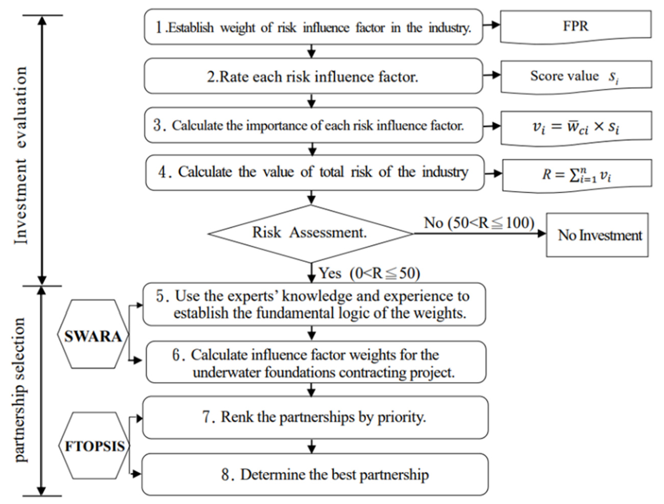
- Investment Evaluation Model (IEM):
- 2.
- Partner Selection Model (PSM):
2. Literature Review
2.1. Risk Factors of Investment in Offshore Wind Power Industry
2.2. Discussion on Factors Affecting Investment Risks in Offshore Wind Power Industry
2.3. Fuzzy Preference Relations (FPR)
- 3.
- Multiplicative Preference Relation (MPR):
- 4.
- Additive Preference Relationship:
2.4. Step-Wise Weight Assessment Ratio Analysis (SWARA)
- Step 1.
- Determine the order of each criterion:Sort the influence and scores in descending order according to the importance of the conditions;
- Step 2.
- The relative importance of the criteria:
- Step 3.
- Recalculate the coefficient of weight;Starting from the second criterion, experts have pointed out that the ratio of standard j to the previous (j-1) attribute is called the relative importance of the average value and is expressed as Sj;
- Step 4.
- Calculate the initial weight shown as follows;
- Step 5.
- Calculate the final weight shown as follows.
2.5. Fuzzy Technique for Order Preference by Similarity to Ideal Solution (FTOPSIS)
3. Establishing a Model for Investment Evaluation and Partner Selection in the Offshore Wind Power Foundations Industry
3.1. Investment Evaluation Model (IEM)
3.1.1. Evaluation Model Construction Process
3.1.2. Calculating the Weights of Investment Risk Factors in the Offshore Wind Power Industry
- Step 1.
- Define linguistic variables:
- Step 2.
- Expert questionnaire:
- Step 3.
- Build the MPR matrix:
- Step 4.
- Establish the values of the other elements in the upper right corner of the MPR matrix:
- Step 5.
- Establish the value of the lower left element of the diagonal line of the MPR matrix Ak [21]:
- Step 6.
- Find the maximum value zk in the MPR matrix Ak.
- Step 7.
- Convert the MPR matrix Ak into a consistent MPR matrix Ck
- Step 8.
- Convert the consistent MPR matrix Ck into the FPR matrix Bk. Convert the MPR matrix Ck, of which the value range is within (1/9,9). Use Equation (6) to convert to an FPR matrix Bk with a value range within (0, 1) [21].
- Step 9.
- Average the respondents’ pairwise matrix FPR:
- Step 10.
- Normalize the FPR matrix obtained from step 9 [21].
- Step 11.
- Obtain the weight of each factor:
3.1.3. Rating the Risk Influence Factors
3.2. Partner Selection Model (PSM)
3.2.1. Calculate the Weight of the Influence Factors
- Step 1.
- Importance ranking:
- Step 2.
- Importance comparison:
- Step 3.
- Calculate the relative importance function according to Formula (12) [34]:
- Step 4.
- Calculate the initial weight according to Formula (13) [34]:
- Step 5.
- Obtain the final weight according to Formula (14) [34]:
3.2.2. Establish the Most Suitable Partnership Ranking
- Step 1.
- Use of linguistic variables to evaluate the candidates:
- Step 2.
- Establish fuzzy decision matrix:
- Step 3.
- Establish a normalized fuzzy matrix:
- Step 4.
- Calculate the weighted normalized fuzzy decision matrix:
- Step 5.
- Calculate the fuzzy positive ideal solution and fuzzy negative ideal solution with Equations (19) and (20):
- Step 6.
- Use the measurement method to find the gap between each candidate and the positive and negative ideal solutions [69]:
- Step 7.
- Calculate the correlation coefficient (CCi) and rank the order of the alternatives:
4. Case Analysis and Verification of Decision-Making Model
4.1. Case Background
4.1.1. The Case of Offshore Wind Farm Development
- Project content: The total installation capacity of this project is 300 MW. Single-unit capacities of 5.2 MW, 6 MW, 8 MW, and 9.5 MW wind turbines are planned. Individual wind turbines are planned with structural support from the bottom of the sleeves (jacket-type).
- Project location: Located in the western offshore waters of Lugang District, Changbin Industrial Zone, Changhua County, the closest distance from the shore is about 16 km; the water depth is about 37–49 m.
- Project benefits: The financial assessment of the cost benefit analysis of this project is passed. The results reflect the growing trend of large-scale wind turbines and the anticipated positive results of the cost benefit analysis.
- Project contracting (wind turbine substructure): The contracting is expected to start in April 2021 for a 3-month duration and to be completed by the end of June 2021.
- Preparatory work for the lower structure of the wind turbines: The preparatory work is expected to start in July 2021 for a 9-month duration and to be completed by the end of March 2022.
- Production of the wind turbine substructure: The production is expected to start in April 2022. Preliminary assessment indicates that a sleeve (jacket-type) substructure takes about 10 to 14 days to manufacture, so 50 sleeve substructures can be produced per year on average. Based on this production rate, completion can be expected by the end of March 2024.
- Construction of the wine turbine substructure: Installation is planned to be carried out from April to September every year, to avoid the northeast monsoon season. The construction is scheduled to start in April 2023 and the installation of all the wind turbine substructures will be completed by the middle of 2024.
- Project cost: The amount of investment of each plan is shown in Table 7.
4.1.2. Profiles of Potential Partners in the Underwater Foundations Industry
4.2. Preliminary Investment Assessment
4.2.1. FPR Weight Calculation of Risk Impact Factors
- Step 1.
- Questionnaire survey:
- Step 2.
- Establish MPR matrix A according to the quantitative value of the evaluation result:
- Step 3.
- Calculate the consistent MPR matrix:
- Step 4.
- Convert to FPR matrix:
- Step 5.
- Average the respondents’ paired FPR matrices:
- Step 6.
- Obtain the weight of each risk influence factor:
4.2.2. Rating the Influence Factors of Industrial Investment Risk
4.3. Project Partner Selection Stage
4.3.1. Calculate the Weight Value of the Selection Influence Factor
- Step 1.
- Importance ranking and importance comparison:
- Step 2.
- Calculate the relative importance function according to Formula (12), as shown in Table 19.

| New Ranking | Sj | |
|---|---|---|
| F6 Ability to Fulfill on Schedule | – | 1 |
| F3 Technical Ability | 0.15 | 1.15 |
| F7 Financial Capability | 0.15 | 1.15 |
| F5 Risk Management and Resilience | 0.05 | 1.05 |
| F9 Management Ability | 0.10 | 1.10 |
| F2 Track Record | 0.15 | 1.15 |
| F4 Quality of Staff | 0.10 | 1.10 |
| F13 Availability and Performance of Ships and Equipment | 0.15 | 1.15 |
| F10 Pricing and Cost | 0.10 | 1.10 |
| F8 Market Viability | 0.05 | 1.05 |
| F11 Information Sharing | 0.05 | 1.05 |
| F12 Research and Innovation | 0.05 | 1.05 |
| F1 Company Reputation | 0.05 | 1.05 |
- Step 3.
- Calculate the initial weight according to Formula (13), as shown in Table 20.
| New Ranking | Sj | ||
|---|---|---|---|
| F6 Ability to Fulfill on Schedule | - | 1 | 1 |
| F3 Technical Ability | 0.15 | 1.15 | 0.870 |
| F7 Financial Capability | 0.15 | 1.15 | 0.757 |
| F5 Risk Management and Resilience | 0.05 | 1.05 | 0.721 |
| F9 Management Ability | 0.10 | 1.10 | 0.655 |
| F2 Track Record | 0.15 | 1.15 | 0.570 |
| F4 Quality of Staff | 0.10 | 1.10 | 0.518 |
| F13 Availability and Performance of Ships and Equipment | 0.15 | 1.15 | 0.450 |
| F10 Pricing and Cost | 0.10 | 1.10 | 0.410 |
| F8 Market Viability | 0.05 | 1.05 | 0.390 |
| F11 Information Sharing | 0.05 | 1.05 | 0.371 |
| F12 Research and Innovation | 0.05 | 1.05 | 0.353 |
| F1 Company Reputation | 0.05 | 1.05 | 0.336 |
- Step 4.
- Obtain the final weight according to Formula (14), as shown in Table 21.
| New Ranking | Sj | |||
|---|---|---|---|---|
| F6 Ability to Fulfill on Schedule | - | 1 | 1 | 0.135 |
| F3 Technical Ability | 0.15 | 1.15 | 0.870 | 0.118 |
| F7 Financial Capability | 0.15 | 1.15 | 0.757 | 0.102 |
| F5 Risk Management and Resilience | 0.05 | 1.05 | 0.721 | 0.098 |
| F9 Management Ability | 0.10 | 1.10 | 0.655 | 0.089 |
| F2 Track Record | 0.15 | 1.15 | 0.570 | 0.077 |
| F4 Quality of Staff | 0.10 | 1.10 | 0.518 | 0.070 |
| F13 Availability and Performance of Ships and Equipment | 0.15 | 1.15 | 0.450 | 0.061 |
| F10 Pricing and Cost | 0.10 | 1.10 | 0.410 | 0.054 |
| F8 Market Viability | 0.05 | 1.05 | 0.390 | 0.053 |
| F11 Information Sharing | 0.05 | 1.05 | 0.371 | 0.050 |
| F12 Research and Innovation | 0.05 | 1.05 | 0.353 | 0.048 |
| F1 Company Reputation | 0.05 | 1.05 | 0.336 | 0.045 |
| Subtotal | 7.401 | 1 |
- Step 5.
- Calculate the arithmetic average of the weights from all the experts:
4.3.2. Selection of the Most Suitable Partnership
- Step 1.
- Expert Evaluation:
- Step 2.
- Establish fuzzy decision matrix:
- Step 3.
- Establish a normalized fuzzy decision matrix:
- Step 4.
- Establish a weighted normalized fuzzy decision matrix:
- Step 5.
- Calculate the fuzzy positive and negative ideal solution vectors:
- Step 6.
- Calculating the positive and negative degrees of separation:
- Step 7.
- Calculate and sort the coefficients of determination:
4.4. Determining the Best Decision Plan
5. Conclusions and Suggestions
5.1. Conclusions
- Previous research on evaluation models mostly explored the choice of a single-frame evaluation model or a single-perspective evaluation structure, which could cause deviations in the evaluation results. This study, on the other hand, establishes a different composite evaluation model and successfully integrates several evaluation methods so as to obtain a more objective evaluation result.
- The study applied FPR to calculate the weight of the risk factors, along with the scores, to determine investment risk in the offshore wind power foundations industry. In addition, SWARA was adopted to calculate the weight of partners’ criteria, followed by FTOPSIS to select the most suitable partner. The study serves as a valuable reference for the firms in their decision-making process.
- The “Investment Evaluation and Partner Selection Model in the Offshore Wind Power Underwater Foundations Industry” established in this study simplifies what was formerly a lengthy and complicated selection process. Throughout the evaluation process, only decision makers’ intuitive judgement data are required in order to quickly and accurately generate fair and accurate evaluations and recommendations.
- Using the criteria and weights analyzed in this research as a guide, the firms in the supply chain can proactively raise their professional thresholds, whereby they can accelerate the development of offshore wind power and its related industries. Once training and professional skills are acquired, local wind farms in Taiwan can then expand into the Asia-Pacific market going forward.
5.2. Suggestions
- This research only focuses on the underwater basic industries that currently have advantages in offshore wind power localization. Follow-up research can be expanded to other localization projects such as wind turbine components, submarine cables, offshore work ships, and maritime engineering.
- The criteria for the compilation of this study and the scale of potential partners are only discussed based on existing data. After the development of Taiwanese wind farms in the future, more and more updated data will be collected. Follow-up research can be combined with artificial intelligence methods to refine the evaluation model. Besides, the proposed framework relies on risk preference parameters. Since risk preferences vary from person to person, introducing machine learning methods such as neural network and genetic programming to simulate decision preferences can not only improve evaluation efficiency, but also ensure model accuracy, which will be an important future research agenda.
- Due to the small number of wind farms developed and constructed in Taiwan, this study can only use a single case for model verification. It is recommended that future studies explore more cases for model verification and comparison.
Author Contributions
Funding
Institutional Review Board Statement
Informed Consent Statement
Data Availability Statement
Conflicts of Interest
References
- Almutairi, K.; Mostafaeipour, A.; Jahanshahi, E.; Jooyandeh, E.; Himri, Y.; Jahangiri, M.; Issakhov, A.; Chowdhury, S.; Hosseini Dehshiri, S.J.; Hosseini Dehshiri, S.S.; et al. Ranking Locations for Hydrogen Production Using Hybrid Wind-Solar: A Case Study. Sustainability 2021, 13, 4524. [Google Scholar] [CrossRef]
- The Global Wind Energy Council. Taiwan Finally Has What the Whole World Desires. Available online: http://www.asindexing.org/site/software.shtml (accessed on 29 January 2019).
- IEA. Offshore Wind Outlook. Available online: https://www.iea.org/reports/offshore-wind-outlook-2019 (accessed on 20 July 2019).
- Executive Yuan Important Policy. Efforts to Promote Offshore Wind Power to Build Taiwan into Asia’s Offshore Wind Power Technology Industry Clusters. Available online: https://www.ey.gov.tw/Page/5A8A0CB5B41DA11E/9eebb9b8-490b-4357-963fa48a981852a7 (accessed on 2 August 2019).
- Jian, F.; Peng, K.; Lin, W. 2025 after Annual Growth of Offshore Wind Power 1GW. Taiwan News. Available online: https://www.chinatimes.com/newspapers/20190426000292-260202?chdtv (accessed on 2 August 2019).
- Jianxing, L. The Green Treasure of the Taiwan Strait. Available online: https://www.gvm.com.tw/article/42527 (accessed on 12 December 2020).
- Liu, Q.; Sun, Y.; Wu, M. Decision-making methodologies in offshore wind power investments: A review. J. Clean. Prod. 2021, 295, 126459. [Google Scholar] [CrossRef]
- Büyüközkan, G.; Karabulut, Y. Energy project performance evaluation with sustainability perspective. Energy 2017, 119, 549–560. [Google Scholar] [CrossRef]
- Karatop, B.; Taşkan, B.; Adar, E.; Kubat, C. Decision analysis related to the renewable energy investments in Turkey based on a Fuzzy AHP-EDAS-Fuzzy FMEA approach. Comput. Ind. Eng. 2021, 151, 106958. [Google Scholar] [CrossRef]
- Wu, Y.; Xu, C.; Ke, Y.; Li, X.; Li, L. Portfolio selection of distributed energy generation projects considering uncertainty and project interaction under different enterprise strategic scenarios. Appl. Energy 2019, 236, 444–464. [Google Scholar] [CrossRef]
- Karakas, E.; Yildiran, O.V. Evaluation of Renewable Energy Alternatives for Turkey via Modified Fuzzy AHP. Int. J. Energy Econ. Policy 2019, 9, 31–39. [Google Scholar] [CrossRef] [Green Version]
- Nigim, K.; Munier, N.; Green, J. Green Pre-feasibility. MCDM tools to aid communities in prioritizing local viable renewable energy sources. Renew. Energy 2004, 29, 1775–1791. [Google Scholar] [CrossRef]
- Keeley, A.R.; Matsumoto, K. Relative significance of determinants of foreign direct investment in wind and solar energy in developing countries—AHP analysis. Energy Policy 2018, 123, 337–348. [Google Scholar] [CrossRef]
- Ahmad, S.; Tahar, R.M. Selection of renewable energy sources for sustainable development of electricity generation system using analytic hierarchy process: A case of Malaysia. Renew. Energy 2014, 63, 458–466. [Google Scholar] [CrossRef]
- Aragonés-Beltrán, P.; Chaparro-González, F.; Pastor-Ferrando, J.-P.; Pla-Rubio, A. An AHP (Analytic Hierarchy Process)/ANP (Analytic Network Process)-based multi-criteria decision approach for the selection of solar-thermal power plant investment projects. Energy 2014, 66, 222–238. [Google Scholar] [CrossRef]
- Chatzimouratidis, A.I.; Pilavachi, P.A. Technological, economic and sustainability evaluation of power plants using the Analytic Hierarchy Process. Energy Policy 2009, 37, 778–787. [Google Scholar] [CrossRef]
- Lee, A.H.; Chen, H.H.; Kang, H.-Y. Multi-criteria decision making on strategic selection of wind farms. Renew. Energy 2009, 34, 120–126. [Google Scholar] [CrossRef]
- Harker, P.L. Alternative modes of questioning in the analytic hierarchy process. Math. Modeling 1987, 9, 353–360. [Google Scholar] [CrossRef] [Green Version]
- Belton, V.; Gear, A.E. The Legitimacy of Rank Reversal–A Comment. Omega 1985, 13, 227–230. [Google Scholar] [CrossRef]
- Millet, I.; Harker, P.T. Globally effective questioning in the analytic hierarchy process. Eur. J. Oper. Res. 1990, 48, 88–97. [Google Scholar] [CrossRef]
- Herrera-Viedma, E.; Herrera, F.; Chiclana, F.; Luque, M. Some issues on consistency of fuzzy preference relations. Eur. J. Oper. Res. 2004, 154, 98–109. [Google Scholar] [CrossRef]
- Stanek, M.B. Measuring alliance value and risk: A model approach to prioritizing alliance projects. Manag. Decis. 2004, 42, 182–204. [Google Scholar] [CrossRef]
- Duisters, D.; Duysters, G.M.; de Man, A.P. The partner selection process: Steps effectiveness, governance. Int. J. Strateg. Bus. Alliances 2011, 2, 7–25. [Google Scholar] [CrossRef]
- Chen, C.-T.; Lin, C.-T.; Huang, S.-F. A fuzzy approach for supplier evaluation and selection in supply chain management. Int. J. Prod. Econ. 2006, 102, 289–301. [Google Scholar] [CrossRef]
- Fei, T.; Qiao, K.; Lin, Z. GA-BHTR: An improved genetic algorithm for partner selection in virtual manufacturing. Int. J. Prod. Res. 2012, 50, 2079–2100. [Google Scholar]
- Cao, X.; Liu, G.W.; Fu, X.M. Analysis on group decision making of industry-university-research partners choice based on preferences and dynamic intuition. Oper. Res. Manag. Sci. 2013, 22, 33–41. [Google Scholar]
- You, D.M.; Huang, X.Z. Partner selection and evaluation of radical technological innovation. Syst. Eng. 2014, 32, 99–103. [Google Scholar]
- Guoyuan, H.; Wei, C.; Zhijun, F. Selection of enterprise’s cooperative innovation partners-based on PSO fixed weight and ameliorated TOPSIS method. Sci. Res. Manag. 2014, 35, 119–126. [Google Scholar]
- Shenglan, S. Multi-attribute decision making mode of dynamic alliance partner selection based on fuzzy. Oper. Res. Manag. Sci. 2015, 24, 36–40. [Google Scholar]
- Baizhou, L.; Shuo, G. Research on the mutualism partner selection of enterprise collaborative original innovation. J. Harbin Eng. Univ. 2019, 40, 1367–1374. [Google Scholar]
- Keršulienė, V.; Zavadskas, E.K.; Turskis, Z. Selection of rational dispute resolution method by applying new step-wise weight assessment ratio analysis (SWARA). J. Bus. Econ. Manag. 2010, 11, 243–258. [Google Scholar] [CrossRef]
- Aghdaie, M.H.; Zolfani, S.H.; Zavadskas, E.K. Decision-making in machine tool selection: An integrated approach with SWARA and COPRAS-G methods. Eng. Econ. 2013, 24, 5–17. [Google Scholar]
- Zolfani, S.H.; Yazdani, M.; Zavadskas, E.K. An extended stepwise weight assessment ratio analysis (SWARA) method for improving criteria prioritization process. Soft Comput. 2018, 22, 7399–7405. [Google Scholar] [CrossRef]
- Sushrut, H.; Vinchurkar, B.; Samtani, K. Performance evaluation of the hydropower plants using various Multi-Criteria Decision-Making techniques. Int. J. Eng. Adv. Technol. 2019, 8, 2131–2138. [Google Scholar]
- Chen, C.-T. Extensions of the TOPSIS for group decision-making under fuzzy environment. Fuzzy Sets Syst. 2000, 114, 1–9. [Google Scholar] [CrossRef]
- Ecer, F. Bulanık ortamlarda grup kararı vermeye yardımcı bir yöntem: Fuzzy TOPSIS ve bir uygulama. Dokuz Eylul Univ. J. Fac. Bus. 2006, 7, 77–96. [Google Scholar]
- Zhao, Z.Y.; Hu, J.; Zuo, J. Performance of wind power industry development in China: A DiamondModel study. Renew. Energy 2009, 34, 2883–2891. [Google Scholar] [CrossRef]
- Masini, A.; Menichetti, E. The impact of behavioral factors in the renewable energy investment decision making process: Conceptual framework and empirical findings. Energy Policy 2012, 40, 28–38. [Google Scholar] [CrossRef]
- Salo, O.; Syri, S. What economic support is needed for Arctic offshore wind power? Renew. Sustain. Energy Rev. 2014, 31, 343–352. [Google Scholar] [CrossRef]
- Jin, X.; Zhang, Z.; Shi, X.; Ju, W. A review on wind power industry and corresponding insurance market in China: Current status and challenges. Renew. Sustain. Energy Rev. 2014, 38, 1069–1082. [Google Scholar] [CrossRef]
- Prostean, G.; Badea, A.; Vasar, C.; Octavian, P. Risk Variables in Wind Power Supply Chain. Procedia-Soc. Behav. Sci. 2014, 124, 124–132. [Google Scholar] [CrossRef] [Green Version]
- Balks, M.; Breloh, P. Risk assessment for investments in offshore wind turbines. J. Econ. Policy 2014, 94, 26–33. [Google Scholar]
- Yanshuo, L. Green Energy Industry Risk Management and Insurance Planning-Taking Offshore Wind Power as an Example. Master’s Thesis, Tamkang University, New Taipei City, Taiwan, 2016. [Google Scholar]
- Gatzert, N.; Kosub, T. Risks and risk management of renewable energy projects: The case of onshore and offshore wind parks. Renew. Sustain. Energy Rev. 2016, 60, 982–998. [Google Scholar] [CrossRef]
- Rolik, Y. Risk Management in Implementing Wind Energy Project. Procedia Eng. 2017, 178, 278–288. [Google Scholar] [CrossRef]
- Angelopoulos, D.; Doukas, H.; Psarras, J.; Stamtsis, G. Risk-based analysis and policy implications for renewable energy investments in Greece. Energy Policy 2017, 105, 512–523. [Google Scholar] [CrossRef]
- Liping, X.; Xinhua, L. The British offshore wind power industry chain development of local experience. Build. Known Inf. 2019, 433, 24–27. [Google Scholar]
- Tu, Y. Benefit evaluation for ocean engineering based on grey Euclid model of game compromise. Clust. Comput. 2018, 22, 4625–4630. [Google Scholar] [CrossRef]
- Bayazit, O.; Karpak, B.; Yagci, A. A purchasing decision: Selecting a supplier for a construction company. J. Syst. Sci. Syst. Eng. 2006, 15, 217–231. [Google Scholar] [CrossRef]
- Eriksson, P.E.; Pesamaa, O. Modelling procurement effects on cooperation. Constr. Manag. Econ. 2007, 25, 893–901. [Google Scholar] [CrossRef] [Green Version]
- Taiwan Power Co., Ltd. Study the related technologies of offshore wind power generation planning, environmental assessment, construction, operation, maintenance etc. Overseas Rep. 2007, 1, 38–67. [Google Scholar]
- Mat, N.A.C.; Cheung, Y.; Scheepers, H. Partner Selection: Criteria for Successful Collaborative Network. ACIS 2009, 43, 631–641. [Google Scholar]
- Ministry of Internal Affairs and Construction of the Republic of China. Construction Industry Evaluation Approach. Available online: https://law.moj.gov.tw/LawClass/LawAll.aspx?pcode=D0070144 (accessed on 2 August 2019).
- Watt, D.; Kayis, B.; Willey, K. The relative importance of tender evaluation and contractor selection criteria. Int. J. Proj. Manag. 2010, 28, 51–60. [Google Scholar] [CrossRef]
- Horta, I.; Camanho, A.; Lima, A.F. Design of Performance Assessment System for Selection of Contractors in Construction Industry E-Marketplaces. J. Constr. Eng. Manag. 2013, 139, 910–917. [Google Scholar] [CrossRef]
- Liang, R.; Sheng, Z.; Xu, F.; Wu, C. Bidding Strategy to Support Decision-Making Based on Comprehensive Information in Construction Projects. Discret. Dyn. Nat. Soc. 2016, 2016, 4643630. [Google Scholar] [CrossRef]
- Taiwan Power Co., Ltd. Offshore Wind First Phase of the Project-Demonstration Wind Farm New Construction Tender Documents; Taiwan Power Co., Ltd.: Taipei, Taiwan, 2017. [Google Scholar]
- Tingting, C. Establishment of the Strategic Model of Procurement and Contracting of Offshore Wind Power Marine Engineering-Taking Taiwan as an Example. Master’s Thesis, Department of Construction Engineering, National Taiwan University of Science and Technology, Taipei, Taiwan, 2018. [Google Scholar]
- Xinhua, L. Opportunities in Taiwan’s offshore marine wind power projects and challenges. Constr. Known Inf. 2018, 429, 25–31. [Google Scholar]
- Weixian, L. The Impact of Weather Conditions in the Taiwan Sea on the Establishment and Operation of Offshore wind Power. In Green Finance and Offshore Wind Power Development Risks and Prospects; Institute of Green Energy and Environment, Industrial Technology Research Institute: Hsinchu County, Taiwan, 2018. [Google Scholar]
- Liu, L.; Ran, W. Research on supply chain partner selection method based on BP neural network. Neural Comput. Appl. 2019, 32, 1543–1553. [Google Scholar] [CrossRef]
- Wind Taiwan Offshore Wind Power Magazine. Taking One Step Further in Offshore Wind Taiwan Needs to Build a Real Local Wind Farm. Available online: https://www.windtaiwan.com/Article/ArticleDetail/1448 (accessed on 4 February 2020).
- Taiwan Power Company. The Second Phase of Offshore Wind Project Feasibility Study. Available online: https://www.taipower.com.tw/upload/1428/2018082909542479857.pdf (accessed on 12 December 2019).
- Ruilun, S. Discussion on Contracting Strategy of Construction Formwork Project. Master’s Thesis, Fengjia University, Taichung City, Taiwan, 2008. [Google Scholar]
- Zilan, L. Establishment of the Selection Partner Model for International Joint Contract Projects—Taking Engineering Consulting Companies as an Example. Master’s Thesis, National Taiwan University of Science and Technology, Taipei, Taiwan, 2010. [Google Scholar]
- Zhumao, L. Research on MCPM’s Application in Decision-Making of Construction Industry Selection of Subcontractors. Master’s Thesis, National Taiwan University of Science and Technology, Taipei, Taiwan, 2011. [Google Scholar]
- Shangde, K. Multi- criteria Prospective Model of General Contractor Selection for Construction Projects. Ph.D. Thesis, National Taiwan University of Science and Technology, Taipei, Taiwan, 2011. [Google Scholar]
- Hwang, C.L.; Yoon, K. Multiple Attribute Decision Making Methods and Applications: A State of the Art Survey; Springer: Berlin/Heidelberg, Germany, 1981. [Google Scholar]
- Wang, Y.J.; Lee, H.S.; Lin, K. Fuzzy TOPSIS for multi-criteria decision-making. Int. Math 2003, 3, 367–379. [Google Scholar]
- Hastak, M.; Shaked, A. ICRAM-1: Model for International Construction Risk Assessment. J. Manag. Eng. 2000, 16, 59–69. [Google Scholar] [CrossRef]

| Sn | Zhao et al. [37] | Masinia et al. [38] | Salo et al. [39] | Jin et al. [40] | Prostean et al. [41] | Balks et al. [42] | Lin Yanshuo [43] | Gatzert et al. [44] | Rolik et al. [45] | Dimitrios et al. [46] | Xu et al. [47] | Tu et al. [48] | Frq | |
|---|---|---|---|---|---|---|---|---|---|---|---|---|---|---|
| Factor | ||||||||||||||
| 1 | Policy risk | ✓ | ✓ | ✓ | ✓ | ✓ | ✓ | ✓ | ✓ | ✓ | ✓ | 10 | ||
| 2 | Fair bidding policy | ✓ | ✓ | ✓ | 3 | |||||||||
| 3 | Economic incentives | ✓ | ✓ | ✓ | ✓ | ✓ | 5 | |||||||
| 4 | Preferential tariff rate | ✓ | ✓ | ✓ | ✓ | ✓ | ✓ | 6 | ||||||
| 5 | Financing risk | ✓ | ✓ | ✓ | ✓ | ✓ | ✓ | ✓ | ✓ | ✓ | 9 | |||
| 6 | Financial incentives | ✓ | ✓ | ✓ | 3 | |||||||||
| 7 | Technology development risk | ✓ | ✓ | ✓ | ✓ | ✓ | ✓ | ✓ | ✓ | ✓ | ✓ | ✓ | ✓ | 12 |
| 8 | Wind power specification | ✓ | ✓ | ✓ | 3 | |||||||||
| 9 | Wind power training | ✓ | ✓ | 2 | ||||||||||
| 10 | Social risk | ✓ | ✓ | ✓ | 3 | |||||||||
| 11 | Market risk | ✓ | ✓ | ✓ | ✓ | ✓ | ✓ | ✓ | ✓ | ✓ | 9 | |||
| 12 | Investor experience | ✓ | ✓ | ✓ | ✓ | 4 | ||||||||
| 13 | Financial risk | ✓ | ✓ | ✓ | ✓ | ✓ | ✓ | 5 | ||||||
| 14 | Estimated investment profit | ✓ | ✓ | ✓ | ✓ | ✓ | ✓ | 6 | ||||||
| 15 | Construction risk | ✓ | ✓ | ✓ | ✓ | ✓ | ✓ | 6 | ||||||
| 16 | Country risk | ✓ | ✓ | ✓ | ✓ | ✓ | 5 | |||||||
| 17 | Risk of natural disasters | ✓ | ✓ | ✓ | ✓ | ✓ | ✓ | 6 | ||||||
| 18 | Competitive risk | ✓ | ✓ | ✓ | ✓ | ✓ | 5 | |||||||
| 19 | Logistics risk | ✓ | ✓ | ✓ | ✓ | 4 | ||||||||
| 20 | Partnership risk | ✓ | ✓ | ✓ | ✓ | ✓ | ✓ | 6 | ||||||
| 21 | Contract risk | ✓ | ✓ | ✓ | ✓ | 4 | ||||||||
| 22 | Construction period risk | ✓ | ✓ | 2 | ||||||||||
| 23 | Supply chain risk | ✓ | ✓ | ✓ | ✓ | 4 | ||||||||
| 24 | Environmental risk | ✓ | 1 | |||||||||||
| 25 | Risk transfer-insurance | ✓ | 1 | |||||||||||
| 26 | Developer’s credit risk | ✓ | ✓ | ✓ | 3 |
| Sn | Authors | Bayazit et al. [49] | Eriksson et al. [50] | TPC 1 [51] | Mat et al. [52] | ROC CPAMI [53] | Watt et al. [54] | Horta et al. [55] | Liang et al. [56] | TPC 2 [57] | Cao Tingting [58] | Lin Hsinua [59] | Lu Weishien [60] | Liuet al.[61] | Neptune [62] | TPC3 [63] | Frq | |
|---|---|---|---|---|---|---|---|---|---|---|---|---|---|---|---|---|---|---|
| Factor | ||||||||||||||||||
| 1 | Company reputation | ✓ | ✓ | ✓ | ✓ | ✓ | ✓ | ✓ | 7 | |||||||||
| 2 | Track records | ✓ | ✓ | ✓ | ✓ | ✓ | ✓ | ✓ | ✓ | ✓ | ✓ | ✓ | ✓ | ✓ | ✓ | 14 | ||
| 3 | Integration capabilities | ✓ | ✓ | ✓ | ✓ | 5 | ||||||||||||
| 4 | Technical ability | ✓ | ✓ | ✓ | ✓ | ✓ | ✓ | ✓ | ✓ | ✓ | ✓ | ✓ | ✓ | ✓ | ✓ | 14 | ||
| 5 | Quality of staff | ✓ | ✓ | ✓ | ✓ | ✓ | ✓ | ✓ | ✓ | ✓ | 9 | |||||||
| 6 | Group culture | ✓ | ✓ | ✓ | 3 | |||||||||||||
| 7 | Willingness to cooperate | ✓ | ✓ | ✓ | ✓ | ✓ | ✓ | 6 | ||||||||||
| 8 | Risk management | ✓ | ✓ | ✓ | ✓ | ✓ | ✓ | ✓ | 7 | |||||||||
| 9 | Performance ability | ✓ | ✓ | ✓ | ✓ | ✓ | ✓ | ✓ | ✓ | ✓ | 9 | |||||||
| 10 | Financial capability | ✓ | ✓ | ✓ | ✓ | ✓ | ✓ | ✓ | ✓ | ✓ | ✓ | ✓ | 11 | |||||
| 11 | Market viability | ✓ | ✓ | ✓ | ✓ | ✓ | ✓ | ✓ | 8 | |||||||||
| 12 | Management ability | ✓ | ✓ | ✓ | ✓ | ✓ | ✓ | ✓ | ✓ | ✓ | 9 | |||||||
| 13 | Pricing and cost | ✓ | ✓ | ✓ | ✓ | ✓ | ✓ | ✓ | ✓ | ✓ | 9 | |||||||
| 14 | Information sharing | ✓ | ✓ | ✓ | ✓ | ✓ | ✓ | ✓ | 7 | |||||||||
| 15 | Research and innovation | ✓ | ✓ | ✓ | ✓ | ✓ | ✓ | ✓ | ✓ | 8 | ||||||||
| 16 | Organization size | ✓ | ✓ | ✓ | ✓ | ✓ | 5 | |||||||||||
| 17 | Ship quantity rerformance | ✓ | ✓ | ✓ | ✓ | ✓ | ✓ | ✓ | 7 | |||||||||
| 18 | Negotiating ability | ✓ | ✓ | 2 | ||||||||||||||
| 19 | Construction quality | ✓ | ✓ | ✓ | ✓ | ✓ | ✓ | 6 | ||||||||||
| 20 | Safety management | ✓ | ✓ | ✓ | ✓ | ✓ | 6 | |||||||||||
| 21 | Port facility energy | ✓ | 1 | |||||||||||||||
| 22 | Communication ability | ✓ | 1 | |||||||||||||||
| Linguistic Variables | Importance |
|---|---|
| Absolutely more important | 9 |
| Very strongly more important | 7 |
| Strongly more important | 5 |
| Weakly more important | 3 |
| Equally important | 1 |
| Weakly less important | 1/3 |
| Strongly less important | 1/5 |
| Very strongly less important | 1/7 |
| Absolutely less important | 1/9 |
| Degree of Risk | Definition | Score |
|---|---|---|
| Lowest risk | Lowest probability, lowest severity | 0 |
| Lower risk | Lower probability, lower severity | 25 |
| Moderate risk | Moderate probability, moderate severity | 50 |
| Higher risk | Higher probability, higher severity | 75 |
| Highest risk | Highest probability, highest severity | 100 |
| Item | Influence Factor | Importance Ranking | ||||
|---|---|---|---|---|---|---|
| F1 | Company Reputation | - | - | - | - | - |
| F2 | Track Record/Past Performance | - | - | - | - | - |
| F3 | Technical Ability | - | - | - | - | - |
| F4 | Quality of Staff | - | - | - | - | - |
| F5 | Risk Management and Resilience | - | - | - | - | - |
| F6 | Ability to Fulfill on Schedule | - | - | - | - | - |
| F7 | Financial Capability | - | - | - | - | - |
| F8 | Market Viability | - | - | - | - | - |
| F9 | Management Ability | - | - | - | - | - |
| F10 | Pricing and Cost | - | - | - | - | - |
| F11 | Information Sharing | - | - | - | - | - |
| F12 | Research and Innovation | - | - | - | - | - |
| F13 | Availability and Performance of Ships and Equipment | - | - | - | - | - |
| Linguistic the Variables | Triangular Fuzzy Numbers |
|---|---|
| Very poor (VP) | (0, 0, 1) |
| Poor (P) | (0, 1, 3) |
| Mildly poor (MP) | (1, 3, 5) |
| Fair (F) | (3, 5, 7) |
| Mildly good (MG) | (5, 7, 9) |
| Good (G) | (7, 9, 10) |
| Very good (VG) | (9, 10, 10) |
| Underwater Foundations | Piles | Underwater Structure Installation | |
|---|---|---|---|
| 5.2 MW (57 units) | 230 million | 150 million | 130 million |
| 6 MW (50 units) | 300 million | 140 million | 140 million |
| 8 MW (37 units) | 240 million | 90 million | 90 million |
| 9.5 MW (31 units) | 260 million | 80 million | 90 million |
| Number | Company Features |
|---|---|
| P1 | 1. P1 is a world renowned offshore wind farm marine engineering and construction company with turnkey experience and technology. It was born of a merger between GeoSea (DEME Group) and Taiwan’s largest shipbuilding company, providing construction and maintenance services for offshore wind power industrial vessels. To complay with the localization policy, the company can mobilize domestic fleets, including large barges and tugboats. It can also meet the transporting and installation capacity of offshore wind farms in Taiwan. 2. P1 is the first company in Taiwan that provides engineering, procurement, construction, and installation services. It imports GeoSea’s marine engineering technology and management experience, and dispatches GeoSea’s fleet for support. 3. GeoSea has successfully completed 73 offshore wind power projects. |
| P2 | 1. Established more than 40 years ago, P2 Construction Company has a proven track record of marine engineering and ships. In compliance with the government’s new energy projects and industrial localization policy, a subsidiary was established, which joins in cooperation with the UK’s High Speed Transfers (HST) for training and SMS management system technology transfer. 2. In 2019, five more offshore wind turbines were purchased and the fleet became 100% Taiwanese, which met the government’s expectations of localization. An investment of 30 million US dollars is planned in the next 5 years for the introduction and setup of a cabin simulation training center, a platform to train more local crews via simulation and practice. 3. With more than 300 employees and 100 full-time crew members, over 40 work vessels, and the largest domestic marine engineering fleet, P2 Construction Company is the largest maritime construction engineering company in Taiwan. |
| P3 | 1. P3 Maritime Engineering is a joint venture company established by Boskalis, the world’s largest maritime engineering company, and a local Taiwanese construction company. 2. With over 100 years of maritime engineering experience, more than 700 professional ships, and over 9500 professionals with a track record on over 100 offshore wind farm projects worldwide, Boskalis has 30 years of on-site maritime cooperation with P3 Construction in Taiwan and the Asia-Pacific region. 3. Through Boskalis’ experience with many successful offshore wind power projects in Europe, along with P3’s local maritime engineering knowledge in Taiwan, the partnership is able to offer services to Taiwan’s wind farm projects such as engineering design; engineering, procurement, construction and installation (EPCI); manufacturing; transportation and installation; seabed renovation; maritime survey, wind farms decommissioning; etc. |
| Evaluation Factor | Absolutely More Important | Very Strongly More Important | Strongly More Important | Weakly More Important | Equally Important | Weakly Less Important | Strongly Less Important | Very Strongly Less Important | Absolutely Less Important | Evaluation Factor |
|---|---|---|---|---|---|---|---|---|---|---|
| Policy risk | ✓ | Preferential tariff rate | ||||||||
| Preferential tariff rate | ✓ | Financing risk | ||||||||
| Financing risk | ✓ | Technological R&D risk | ||||||||
| Technological R&D risk | ✓ | Market risk | ||||||||
| Market risk | ✓ | projected investment profit | ||||||||
| projected investment profit | ✓ | Construction risk | ||||||||
| Construction risk | ✓ | Natural Disaster | ||||||||
| Natural Disaster | ✓ | Financing risk |
| CF1 | CF2 | CF3 | CF4 | CF5 | CF6 | CF7 | CF8 | CF9 | |
|---|---|---|---|---|---|---|---|---|---|
| CF1 | 1.00 | 0.20 | |||||||
| CF2 | 1.00 | 3.00 | |||||||
| CF3 | 1.00 | 5.00 | |||||||
| CF4 | 1.00 | 1.00 | |||||||
| CF5 | 1.00 | 0.14 | |||||||
| CF6 | 1.00 | 1.00 | |||||||
| CF7 | 1.00 | 3.00 | |||||||
| CF8 | 1.00 | 1.00 | |||||||
| CF9 | 1.00 |
| CF1 | CF2 | CF3 | CF4 | CF5 | CF6 | CF7 | CF8 | CF9 | |
|---|---|---|---|---|---|---|---|---|---|
| CF1 | 1.00 | 0.20 | 0.60 | 3.00 | 3.00 | 0.43 | 0.43 | 1.29 | 1 |
| CF2 | 5.00 | 1.00 | 3.00 | 15.00 | 15.00 | 2.14 | 2.14 | 6.43 | 6 |
| CF3 | 1.67 | 0.33 | 1.00 | 5.00 | 5.00 | 0.71 | 0.71 | 2.14 | 2.14 |
| CF4 | 0.33 | 0.07 | 0.20 | 1.00 | 1.00 | 0.14 | 0.14 | 0.43 | 0.43 |
| CF5 | 0.33 | 0.07 | 0.20 | 1.00 | 1.00 | 0.14 | 0.14 | 0.43 | 0.43 |
| CF6 | 2.33 | 0.47 | 1.40 | 7.00 | 7.00 | 1.00 | 1.00 | 3.00 | 3.00 |
| CF7 | 2.33 | 0.47 | 1.40 | 7.00 | 7.00 | 1.00 | 1.00 | 3.00 | 3.00 |
| CF8 | 0.78 | 0.16 | 0.47 | 2.33 | 2.33 | 0.33 | 0.33 | 1.00 | 1.00 |
| CF9 | 0.78 | 0.16 | 0.47 | 2.33 | 2.33 | 0.33 | 0.33 | 1.00 | 1.00 |
| CF1 | CF2 | CF3 | CF4 | CF5 | CF6 | CF7 | CF8 | CF9 | |
|---|---|---|---|---|---|---|---|---|---|
| CF1 | 1.00 | 0.27 | 0.66 | 2.44 | 2.44 | 0.50 | 0.50 | 1.23 | 1.23 |
| CF2 | 3.69 | 1.00 | 2.44 | 9.00 | 9.00 | 1.86 | 1.86 | 4.53 | 4.53 |
| CF3 | 1.51 | 0.41 | 1.00 | 3.69 | 3.69 | 0.76 | 0.76 | 1.86 | 1.86 |
| CF4 | 0.41 | 0.11 | 0.27 | 1.00 | 1.00 | 0.21 | 0.21 | 0.50 | 0.50 |
| CF5 | 0.41 | 0.11 | 0.27 | 1.00 | 1.00 | 0.21 | 0.21 | 0.50 | 0.50 |
| CF6 | 1.99 | 0.54 | 1.31 | 4.85 | 4.85 | 1.00 | 1.00 | 2.44 | 2.44 |
| CF7 | 1.99 | 0.54 | 1.31 | 4.85 | 4.85 | 1.00 | 1.00 | 2.44 | 2.44 |
| CF8 | 0.82 | 0.22 | 0.54 | 1.99 | 1.99 | 0.41 | 0.41 | 1.00 | 1.00 |
| CF9 | 0.82 | 0.22 | 0.54 | 1.99 | 1.99 | 0.41 | 0.41 | 1.00 | 1.00 |
| CF1 | CF2 | CF3 | CF4 | CF5 | CF6 | CF7 | CF8 | CF9 | |
|---|---|---|---|---|---|---|---|---|---|
| CF1 | 0.50 | 0.20 | 0.41 | 0.70 | 0.70 | 0.34 | 0.34 | 0.55 | 0.55 |
| CF2 | 0.80 | 0.50 | 0.70 | 1.00 | 1.00 | 0.64 | 0.64 | 0.84 | 0.84 |
| CF3 | 0.59 | 0.30 | 0.50 | 0.80 | 0.80 | 0.44 | 0.44 | 0.64 | 0.64 |
| CF4 | 0.30 | 0.00 | 0.20 | 0.50 | 0.50 | 0.14 | 0.14 | 0.34 | 0.34 |
| CF5 | 0.30 | 0.00 | 0.20 | 0.50 | 0.50 | 0.14 | 0.14 | 0.34 | 0.34 |
| CF6 | 0.66 | 0.36 | 0.56 | 0.86 | 0.86 | 0.50 | 0.50 | 0.70 | 0.70 |
| CF7 | 0.66 | 0.36 | 0.56 | 0.86 | 0.86 | 0.50 | 0.50 | 0.70 | 0.70 |
| CF8 | 0.45 | 0.16 | 0.36 | 0.66 | 0.66 | 0.30 | 0.30 | 0.50 | 0.50 |
| CF9 | 0.45 | 0.16 | 0.36 | 0.66 | 0.66 | 0.30 | 0.30 | 0.50 | 0.50 |
| CF1 | CF2 | CF3 | CF4 | CF5 | CF6 | CF7 | CF8 | CF9 | |
|---|---|---|---|---|---|---|---|---|---|
| CF1 | 0.500 | 0.704 | 0.567 | 0.673 | 0.633 | 0.585 | 0.565 | 0.619 | 0.573 |
| CF2 | 0.296 | 0.500 | 0.363 | 0.468 | 0.429 | 0.381 | 0.361 | 0.415 | 0.369 |
| CF3 | 0.433 | 0.637 | 0.500 | 0.606 | 0.567 | 0.518 | 0.498 | 0.552 | 0.506 |
| CF4 | 0.327 | 0.532 | 0.394 | 0.500 | 0.461 | 0.413 | 0.392 | 0.447 | 0.400 |
| CF5 | 0.367 | 0.571 | 0.433 | 0.539 | 0.500 | 0.452 | 0.431 | 0.486 | 0.439 |
| CF6 | 0.415 | 0.619 | 0.482 | 0.587 | 0.548 | 0.500 | 0.480 | 0.534 | 0.488 |
| CF7 | 0.435 | 0.639 | 0.502 | 0.608 | 0.569 | 0.520 | 0.500 | 0.554 | 0.508 |
| CF8 | 0.381 | 0.585 | 0.448 | 0.553 | 0.514 | 0.466 | 0.446 | 0.500 | 0.454 |
| CF9 | 0.427 | 0.631 | 0.494 | 0.600 | 0.561 | 0.512 | 0.492 | 0.546 | 0.500 |
| TOTAL | 3.118 | 4.921 | 4.352 | 5.410 | 5.232 | 5.107 | 4.066 | 4.240 | 4.053 |
| CF1 | CF2 | CF3 | CF4 | CF5 | CF6 | CF7 | CF8 | CF9 | Subtotal | Relative Weights | |
|---|---|---|---|---|---|---|---|---|---|---|---|
| CF1 | 0.160 | 0.143 | 0.130 | 0.124 | 0.121 | 0.115 | 0.139 | 0.146 | 0.141 | 1.220 | 0.134 |
| CF2 | 0.095 | 0.102 | 0.083 | 0.087 | 0.082 | 0.075 | 0.089 | 0.098 | 0.091 | 0.801 | 0.088 |
| CF3 | 0.139 | 0.129 | 0.115 | 0.112 | 0.108 | 0.102 | 0.122 | 0.130 | 0.125 | 1.083 | 0.119 |
| CF4 | 0.105 | 0.108 | 0.091 | 0.092 | 0.088 | 0.081 | 0.096 | 0.105 | 0.099 | 0.866 | 0.095 |
| CF5 | 0.118 | 0.116 | 0.100 | 0.100 | 0.096 | 0.088 | 0.106 | 0.115 | 0.108 | 0.946 | 0.104 |
| CF6 | 0.133 | 0.126 | 0.111 | 0.109 | 0.105 | 0.098 | 0.118 | 0.126 | 0.120 | 1.045 | 0.115 |
| CF7 | 0.140 | 0.130 | 0.115 | 0.112 | 0.109 | 0.102 | 0.123 | 0.131 | 0.125 | 1.087 | 0.120 |
| CF8 | 0.122 | 0.119 | 0.103 | 0.102 | 0.098 | 0.091 | 0.110 | 0.118 | 0.112 | 0.975 | 0.107 |
| CF9 | 0.137 | 0.128 | 0.114 | 0.111 | 0.107 | 0.100 | 0.121 | 0.129 | 0.123 | 1.070 | 0.118 |
| Total | 9.092 | 1.000 | |||||||||
| Risk Impact Factor | Expert 1 Score | Expert 2 Score | Expert 3 Score | Average |
|---|---|---|---|---|
| Policy risk | 25 | 50 | 25 | 33.333 |
| Preferential tariff rate | 25 | 25 | 25 | 25 |
| Financing risk | 75 | 50 | 50 | 58.333 |
| Technological development risk | 50 | 50 | 25 | 41.667 |
| Market risk | 50 | 50 | 25 | 41.667 |
| Projected investment profit | 50 | 25 | 50 | 41.667 |
| Construction risk | 75 | 75 | 75 | 75 |
| Natural disaster risk | 50 | 50 | 75 | 58.333 |
| Partnership risk | 25 | 25 | 25 | 25 |
| Risk Influence Factor | Factor Weight (Wci) | Risk Score (si) | Importance (vi) |
|---|---|---|---|
| Policy risk | 0.134 | 33.333 | 4.467 |
| Preferential tariff rate | 0.088 | 25.000 | 2.200 |
| Financing risk | 0.119 | 58.333 | 6.942 |
| Technological development risk | 0.095 | 41.667 | 3.958 |
| Market risk | 0.104 | 41.667 | 4.333 |
| Projected investment profit | 0.115 | 41.667 | 4.792 |
| Construction risk | 0.120 | 75.000 | 9.000 |
| Natural risk | 0.107 | 58.333 | 6.242 |
| Partner risk | 0.118 | 25.000 | 2.950 |
| Overall investment risk value R | 44.884 | ||
| Item | Influence Factor | Importance Ranking | New Ranking | Sj |
|---|---|---|---|---|
| F1 | Company Reputation | 13 | F6 | - |
| F2 | Track Record/Past Performance | 6 | F3 | 0.15 |
| F3 | Technical Ability | 2 | F7 | 0.15 |
| F4 | Quality of Staff | 7 | F5 | 0.05 |
| F5 | Risk Management and Resilience | 4 | F9 | 0.10 |
| F6 | Ability to Fulfill on Schedule | 1 | F2 | 0.15 |
| F7 | Financial Capability | 3 | F4 | 0.10 |
| F8 | Market Viability | 10 | F13 | 0.15 |
| F9 | Management Ability | 5 | F10 | 0.10 |
| F10 | Pricing and Cost | 9 | F8 | 0.05 |
| F11 | Information Sharing | 11 | F11 | 0.05 |
| F12 | Research and Innovation | 12 | F12 | 0.05 |
| F13 | Availability and Performance of Ships and Equipment | 8 | F1 | 0.05 |
| Item | Expert 1 Weights | Expert 2 Weights | Expert 3 Weights | Expert 4 Weights | Average Weights | New Ranking |
|---|---|---|---|---|---|---|
| F1 | 0.045 | 0.103 | 0.070 | 0.081 | 0.075 | 6 |
| F2 | 0.077 | 0.119 | 0.122 | 0.103 | 0.105 | 2 |
| F3 | 0.118 | 0.090 | 0.140 | 0.130 | 0.119 | 1 |
| F4 | 0.070 | 0.081 | 0.052 | 0.061 | 0.066 | 10 |
| F5 | 0.098 | 0.067 | 0.063 | 0.070 | 0.074 | 7 |
| F6 | 0.135 | 0.078 | 0.084 | 0.113 | 0.103 | 3 |
| F7 | 0.102 | 0.058 | 0.055 | 0.074 | 0.072 | 8 |
| F8 | 0.053 | 0.055 | 0.047 | 0.055 | 0.053 | 11 |
| F9 | 0.089 | 0.061 | 0.076 | 0.089 | 0.079 | 5 |
| F10 | 0.054 | 0.074 | 0.096 | 0.048 | 0.068 | 9 |
| F11 | 0.050 | 0.048 | 0.043 | 0.040 | 0.045 | 13 |
| F12 | 0.048 | 0.053 | 0.041 | 0.042 | 0.046 | 12 |
| F13 | 0.061 | 0.113 | 0.111 | 0.094 | 0.095 | 4 |
| Influence Factor | Expert 1 | Expert 2 | Expert 3 | ||||||
|---|---|---|---|---|---|---|---|---|---|
| P1 | P2 | P3 | P1 | P2 | P3 | P1 | P2 | P3 | |
| F1 | 7, 9, 10 | 5, 7, 9 | 5, 7, 9 | 9, 10, 10 | 5, 7, 9 | 7, 9, 10 | 9, 10, 10 | 7, 9, 10 | 9, 10, 10 |
| F2 | 9, 10, 10 | 7, 9, 10 | 9, 10, 10 | 7, 9, 10 | 3, 5, 7 | 7, 9, 10 | 9, 10, 10 | 5, 7, 9 | 9, 10, 10 |
| F3 | 7, 9, 10 | 7, 9, 10 | 5, 7, 9 | 7, 9, 10 | 5, 7, 9 | 5, 7, 9 | 7, 9, 10 | 7, 9, 10 | 7, 9, 10 |
| F4 | 7, 9, 10 | 3, 5, 7 | 5, 7, 9 | 7, 9, 10 | 7, 9, 10 | 7, 9, 10 | 7, 9, 10 | 3, 5, 7 | 5, 7, 9 |
| F5 | 7, 9, 10 | 7, 9, 10 | 3, 5, 7 | 3, 5, 7 | 5, 7, 9 | 7, 9, 10 | 5, 7, 9 | 3, 5, 7 | 7, 9, 10 |
| F6 | 7, 9, 10 | 7, 9, 10 | 7, 9, 10 | 7, 9, 10 | 3, 5, 7 | 5, 7, 9 | 9, 10, 10 | 5, 7, 9 | 5, 7, 9 |
| F7 | 9, 10, 10 | 3, 5, 7 | 3, 5, 7 | 7, 9, 10 | 3, 5, 7 | 3, 5, 7 | 7, 9, 10 | 5, 7, 9 | 5, 7, 9 |
| F8 | 7, 9, 10 | 1, 3, 5 | 1, 3, 5 | 5, 7, 9 | 5, 7, 9 | 5, 7, 9 | 7, 9, 10 | 3, 5, 7 | 9, 10, 10 |
| F9 | 7, 9, 10 | 3, 5, 7 | 1, 3, 5 | 7, 9, 10 | 3, 5, 7 | 5, 7, 9 | 5, 7, 9 | 7, 9, 10 | 5, 7, 9 |
| F10 | 3, 5, 7 | 5, 7, 9 | 5, 7, 9 | 3, 5, 7 | 7, 9, 10 | 3, 5, 7 | 3, 5, 7 | 3, 5, 7 | 7, 9, 10 |
| F11 | 9, 10, 10 | 3, 5, 7 | 5, 7, 9 | 9, 10, 10 | 5, 7, 9 | 5, 7, 9 | 7, 9, 10 | 7, 9, 10 | 9, 10, 10 |
| F12 | 7, 9, 10 | 5, 7, 9 | 5, 7, 9 | 9, 10, 10 | 7, 9, 10 | 9, 10, 10 | 7, 9, 10 | 3, 5, 7 | 9, 10, 10 |
| F13 | 7, 9, 10 | 5, 7, 9 | 3, 5, 7 | 9, 10, 10 | 5, 7, 9 | 7, 9, 10 | 9, 10, 10 | 3, 5, 7 | 7, 9, 10 |
| Plan | Partnership P1 | Partnership P2 | Partnership P3 | |
|---|---|---|---|---|
| Factor | ||||
| F1 | 7, 9.667, 10 | 5, 7.667, 10 | 5, 8.667, 10 | |
| F2 | 7, 9.667, 10 | 3, 7, 10 | 7, 9.667, 10 | |
| F3 | 7, 9, 10 | 5, 8.333, 10 | 5, 7.667, 10 | |
| F4 | 7, 9, 10 | 3, 6.333, 10 | 5, 7.667, 10 | |
| F5 | 3, 7, 10 | 3, 7, 10 | 3, 7.667, 10 | |
| F6 | 7, 9.333, 10 | 3, 7, 10 | 5, 7.667, 10 | |
| F7 | 7, 9.333, 10 | 3, 5.667, 9 | 3, 5.667, 9 | |
| F8 | 5, 8.333, 10 | 1, 5, 9 | 1, 6.667, 10 | |
| F9 | 5, 8.333, 10 | 3, 6.333, 10 | 1, 5.667, 9 | |
| F10 | 3, 5, 7 | 3, 7, 10 | 3, 7, 10 | |
| F11 | 7, 9.667, 10 | 3, 7, 10 | 5, 8, 10 | |
| F12 | 7, 9.333, 10 | 3, 7, 10 | 5, 9, 10 | |
| F13 | 7, 9.667, 10 | 3, 6.333, 9 | 3, 7.667, 10 | |
| Plan | Partnership P1 | Partnership P2 | Partnership P3 | |
|---|---|---|---|---|
| Factor | ||||
| F1 | 0.7, 0.967, 1 | 0.5, 0.767, 1 | 0.5, 0.867, 1 | |
| F2 | 0.7, 0.967, 1 | 0.3, 0.7, 1 | 0.7, 0.967, 1 | |
| F3 | 0.7, 0.9, 1 | 0.5, 0.833, 1 | 0.5, 0.767, 1 | |
| F4 | 0.7, 0.9, 1 | 0.3, 0.633, 1 | 0.5, 0.767, 1 | |
| F5 | 0.3, 0.7, 1 | 0.3, 0.7, 1 | 0.3, 0.767, 1 | |
| F6 | 0.7, 0.933, 1 | 0.3, 0.7, 1 | 0.5, 0.767, 1 | |
| F7 | 0.7, 0.933, 1 | 0.3, 0.567, 0.9 | 0.3, 0.567, 0.9 | |
| F8 | 0.5, 0.833, 1 | 0.1, 0.5, 0.9 | 0.1, 0.667, 1 | |
| F9 | 0.5, 0.833, 1 | 0.3, 0.633, 1 | 0.1, 0.567, 0.9 | |
| F10 | 0.429, 0.6, 1 | 0.333, 0.45, 1 | 0.333, 0.45, 1 | |
| F11 | 0.7, 0.967, 1 | 0.3, 0.7, 1 | 0.5, 0.8, 1 | |
| F12 | 0.7, 0.933, 1 | 0.3, 0.7, 1 | 0.5, 0.9, 1 | |
| F13 | 0.7, 0.967, 1 | 0.3, 0.633, 0.9 | 0.3, 0.767, 1 | |
| Influence Factor | SWARA Weight | Partnership P1 | Partnership P2 | Partnership P3 |
|---|---|---|---|---|
| F1 | 0.075 | 0.053, 0.073, 0.075 | 0.038, 0.058, 0.075 | 0.038, 0.065, 0.075 |
| F2 | 0.105 | 0.074, 0.102, 0.105 | 0.032, 0.074, 0.105 | 0.074, 0.102, 0.105 |
| F3 | 0.119 | 0.083, 0.107, 0.119 | 0.060, 0.099, 0.119 | 0.060, 0.091, 0.119 |
| F4 | 0.066 | 0.046, 0.059, 0.066 | 0.020, 0.042, 0.066 | 0.033, 0.051, 0.066 |
| F5 | 0.074 | 0.022, 0.052, 0.074 | 0.022, 0.052, 0.074 | 0.022, 0.057, 0.074 |
| F6 | 0.103 | 0.072, 0.096, 0.103 | 0.031, 0.072, 0.103 | 0.052, 0.079, 0.103 |
| F7 | 0.072 | 0.050, 0.067, 0.072 | 0.022, 0.041, 0.065 | 0.022, 0.041, 0.065 |
| F8 | 0.053 | 0.027, 0.044, 0.053 | 0.005, 0.027, 0.048 | 0.005, 0.035, 0.053 |
| F9 | 0.079 | 0.040, 0.066, 0.079 | 0.024, 0.050, 0.079 | 0.008, 0.045, 0.071 |
| F10 | 0.068 | 0.029, 0.041, 0.068 | 0.023, 0.031, 0.068 | 0.023, 0.031, 0.068 |
| F11 | 0.045 | 0.032, 0.044, 0.045 | 0.014, 0.032, 0.045 | 0.023, 0.036, 0.045 |
| F12 | 0.046 | 0.032, 0.043, 0.046 | 0.014, 0.032, 0.046 | 0.023, 0.041, 0.046 |
| F13 | 0.095 | 0.067, 0.092, 0.095 | 0.029, 0.060, 0.086 | 0.029, 0.073, 0.095 |
| Vector | |||
|---|---|---|---|
| Factor | |||
| F1 | 0.053, 0.073, 0.075 | 0.038, 0.058, 0.075 | |
| F2 | 0.074, 0.102, 0.105 | 0.032, 0.074, 0.105 | |
| F3 | 0.083, 0.107, 0.119 | 0.060, 0.091, 0.119 | |
| F4 | 0.046, 0.059, 0.066 | 0.020, 0.042, 0.066 | |
| F5 | 0.022, 0.057, 0.074 | 0.022, 0.052, 0.074 | |
| F6 | 0.072, 0.096, 0.103 | 0.031, 0.072, 0.103 | |
| F7 | 0.050, 0.067, 0.072 | 0.022, 0.041, 0.065 | |
| F8 | 0.027, 0.044, 0.053 | 0.005, 0.027, 0.048 | |
| F9 | 0.040, 0.066, 0.079 | 0.008, 0.045, 0.071 | |
| F10 | 0.029, 0.041, 0.068 | 0.023, 0.031, 0.068 | |
| F11 | 0.032, 0.044, 0.045 | 0.014, 0.032, 0.045 | |
| F12 | 0.032, 0.043, 0.046 | 0.014, 0.032, 0.046 | |
| F13 | 0.067, 0.092, 0.095 | 0.029, 0.060, 0.086 | |
| Influence Factor | Partnership P1 | Partnership P2 | Partnership P3 |
|---|---|---|---|
| F1 | 0 | 0.01225 | 0.00981 |
| F2 | 0 | 0.02914 | 0 |
| F3 | 0 | 0.01407 | 0.00924 |
| F4 | 0 | 0.01794 | 0.00883 |
| F5 | 0.00289 | 0.00289 | 0 |
| F6 | 0 | 0.02742 | 0.01517 |
| F7 | 0 | 0.02207 | 0.02207 |
| F8 | 0 | 0.01631 | 0.01371 |
| F9 | 0 | 0.01308 | 0.02665 |
| F10 | 0 | 0.00671 | 0.00671 |
| F11 | 0 | 0.01249 | 0.00458 |
| F12 | 0 | 0.01217 | 0.00529 |
| F13 | 0 | 0.02915 | 0.02454 |
| 0.00289 | 0.21569 | 0.14660 |
| Influence Factor | Partnership P1 | Partnership P2 | Partnership P3 |
|---|---|---|---|
| F1 | 0.01225 | 0 | 0.00404 |
| F2 | 0.02914 | 0 | 0.02914 |
| F3 | 0.01619 | 0.00462 | 0 |
| F4 | 0.01794 | 0 | 0.03271 |
| F5 | 0 | 0 | 0.00289 |
| F6 | 0.002742 | 0 | 0.01277 |
| F7 | 0.02207 | 0 | 0 |
| F8 | 0.01631 | 0 | 0.00548 |
| F9 | 0.02665 | 0.01072 | 0 |
| F10 | 0.00671 | 0 | 0 |
| F11 | 0.01249 | 0 | 0.00566 |
| F12 | 0.01217 | 0 | 0.00735 |
| F13 | 0.02915 | 0 | 0.00911 |
| () | 0.22849 | 0.01534 | 0.10915 |
| Plan | Partnership P1 | Partnership P2 | Partnership P3 | |
|---|---|---|---|---|
| Factor | ||||
| Positive degree of separation () | 0.00289 | 0.21569 | 0.14660 | |
| Negative degree of separation () | 0.22849 | 0.01534 | 0.10915 | |
| Coefficient of determination () | 0.98751 | 0.06640 | 0.42678 | |
| Ranking | 1 | 3 | 2 | |
Publisher’s Note: MDPI stays neutral with regard to jurisdictional claims in published maps and institutional affiliations. |
© 2021 by the authors. Licensee MDPI, Basel, Switzerland. This article is an open access article distributed under the terms and conditions of the Creative Commons Attribution (CC BY) license (https://creativecommons.org/licenses/by/4.0/).
Share and Cite
Cheng, M.-Y.; Wu, Y.-F. Investment Evaluation and Partnership Selection Model in the Offshore Wind Power Underwater Foundations Industry. J. Mar. Sci. Eng. 2021, 9, 1371. https://doi.org/10.3390/jmse9121371
Cheng M-Y, Wu Y-F. Investment Evaluation and Partnership Selection Model in the Offshore Wind Power Underwater Foundations Industry. Journal of Marine Science and Engineering. 2021; 9(12):1371. https://doi.org/10.3390/jmse9121371
Chicago/Turabian StyleCheng, Min-Yuan, and Yung-Fu Wu. 2021. "Investment Evaluation and Partnership Selection Model in the Offshore Wind Power Underwater Foundations Industry" Journal of Marine Science and Engineering 9, no. 12: 1371. https://doi.org/10.3390/jmse9121371
APA StyleCheng, M.-Y., & Wu, Y.-F. (2021). Investment Evaluation and Partnership Selection Model in the Offshore Wind Power Underwater Foundations Industry. Journal of Marine Science and Engineering, 9(12), 1371. https://doi.org/10.3390/jmse9121371