A Scheme for Estimating Time-Varying Wind Stress Drag Coefficient in the Ekman Model with Adjoint Assimilation

Abstract

In this study, the time-varying wind stress drag coefficient in the Ekman model was inverted by the cubic spline interpolation scheme based on the adjoint method. Twin experiments were carried out to investigate the influences of several factors on inversion results, and the conclusions were (1) the inverted distributions with the cubic spline interpolation scheme were in good agreement with the prescribed distributions of the wind stress drag coefficients, and the cubic spline interpolation scheme was superior to direct inversion by the model scheme and Cressman interpolation scheme; (2) the cubic spline interpolation scheme was more advantageous than the Cressman interpolation scheme even if there is moderate noise in the observations. The cubic spline interpolation scheme was further validated in practical experiments where Ekman currents and wind speed derived from mooring data of ocean station Papa were assimilated. The results demonstrated that the variation of the time-varying wind stress drag coefficient with time was similar to that of wind speed with time, and a more accurate inversion result could be obtained by the cubic spline interpolation scheme employing appropriate independent points. Overall, this study provides a potential way for efficient estimation of time-varying wind stress drag coefficient.

1. Introduction

Wind stress over the sea surface is a primary driving force of upper ocean circulation and ocean surface waves and is an important mechanism by which the atmosphere conveys momentum to the ocean. Therefore, the exact estimation of wind stress is important for the simulation and forecasting of atmospheric and oceanic processes [1]. Meanwhile, wind stress is a key parameter for understanding physical processes in both the atmosphere and ocean, whose determination is important for coupled ocean–atmosphere modeling [2].

Usually, wind stress is parameterized by the wind stress drag coefficient (WSDC). It has long been recognized that the drag coefficient of the sea surface does not depend on wind speed alone, while it has been highlighted that the wind drag coefficient strongly depends on the sea roughness [3,4]. In previous studies, the WSDC was usually assumed to be a constant [5], considered as a linear function with respect to wind speed [6], or further believed to be a nonlinear function with respect to wind speed [7,8]. At present, it is widely accepted that wind stress coefficients vary nonlinearly with wind speed (and thus with time)—especially at high wind speeds [9,10]. Some scholars have found that spatially and temporally varying WSDC fields are needed in a variety of climate and air–sea interaction studies [11,12]. In particular, with the improvement of the time resolution of the model, it is meaningful to study the WSDC with daily variations. The determination of the WSDC is a difficult problem in the field of marine science and atmospheric science because of the interaction between air and sea; this difficulty stems from the problem of turbulence. The turbulence problem is difficult to solve because of its variability in time and space. Ocean observations at near-inertial frequencies show that the turbulent closure model is better at predicting wind speed than the plate model [13]. There are a variety of options for turbulent closure models, such as models depending on Richardson number, k-ε model, M-Y model, Prandtl mixed-length model, KPP model, etc., which play important roles in different regions and different events [14,15,16,17,18]. However, as the ocean environment often changes with space and time, and the observation data are insufficient, the applications of various turbulence models are easily limited. Specifically, the parameters calculated by different models vary greatly, and few models can be accurately applied to all sea areas or problems in the world.

During recent decades, data assimilation has played an important role in the determination of unknown parameters. The process that the parameters are estimated by—assimilating observations with a data assimilation method—is known as parameter estimation. The adjoint method is a powerful tool for parameter estimation, which has been widely used by many scholars. Zhang et al. [19] successfully explored how eddy viscosity is developed with varying wind fields, but did not consider the WSDC. Cao et al. [20] proposed an estimation scheme to evaluate the eddy viscosity profile (EVP) at the bottom of the Ekman boundary layer based on the adjoint method. Zhang et al. [21] successfully inverted the time-varying vertical eddy viscosity coefficients in the Ekman model and also found that the inversion results were much more sensitive to the observations in the upper layers.

In order to improve the computational efficiency and accuracy of parameter estimation, independent point (IP) schemes were used by some scholars in the adjoint method [22,23,24]. The so-called IP scheme is where the WSDCs at some selected IPs are taken as control variables and those at other points are calculated by interpolating values at IPs. There are many interpolation schemes, such as the Cressman interpolation based on linear interpolation. However, the Cressman that was interpolation traditionally used in the IP scheme can result in unsmooth curves. Meanwhile, we found that the cubic spline interpolation (CSI) scheme was often used in practice because of its favorable smoothness and continuity [25,26,27,28]. Therefore, we try to use the CSI instead of linear interpolation to invert the time-varying WSDC in an Ekman model. We aim to improve the simulation capability of the model and provide a reference for the selection of WSDCs in other ocean models. In order to verify the feasibility and accuracy of the CSI scheme, twin experiments and practical experiments are conducted.

The organization of this paper is as follows: In Section 2, the numerical model and CSI scheme are introduced. In Section 3, a series of twin experiments are carried out to verify the feasibility of the CSI scheme. In Section 4, practical experiments are carried out to verify the inverted effect of the CSI scheme. Finally, conclusions are given in Section 5.

2. Numerical Model

2.1. Governing Equations (Forward Model)

In this paper, the Ekman model [29] with time-varying WSDC on the sea surface is used, and its governing equations are:

$$\left\{\begin{array}{c}\frac{\partial u}{\partial t}-fv=\frac{\partial }{\partial z}\left(A\frac{\partial u}{\partial z}\right),\\ \frac{\partial v}{\partial t}+fu=\frac{\partial }{\partial z}\left(A\frac{\partial v}{\partial z}\right).\end{array}\right.$$

(1)

The boundary conditions are

$${\left.\frac{\partial u}{\partial z}\right|}_{z=0}=\frac{C_d}{A}\cdot \frac{{\rho }_a}{{\rho }_w}\sqrt{u_a^2+v_a^2}{u}_a,{\left.\frac{\partial v}{\partial z}\right|}_{z=0}=\frac{C_d}{A}\cdot \frac{{\rho }_a}{{\rho }_w}\sqrt{u_a^2+v_a^2}{v}_a.$$

(2)

$$A{\left.\frac{\partial u}{\partial z}\right|}_{z=-H_0}=0,\begin{array}{cc}& \end{array}\begin{array}{cc}& \begin{array}{cc}& \end{array}\end{array}A{\left.\frac{\partial v}{\partial z}\right|}_{z=-H_0}=0.$$

(3)

The initial conditions are:

$${\left.u\right|}_{t=0}=u_0,\begin{array}{cc}& \begin{array}{cc}\begin{array}{cc}& \end{array}& \end{array}\end{array}{\left.v\right|}_{t=0}=v_0.$$

(4)

where $t$ is the time; $z$ is the water depth, and the vertically upward direction of the z-axis is positive, with $z=0$ at the ocean surface; $u$ (positive to the east) and $v$ (positive to the north) are the horizontal velocity components; $f$ is the Coriolis parameter, which is set as a constant in this model; A is the eddy viscosity coefficient; $C_d$ is the time-varying WSDC; ${\rho }_a$ and ${\rho }_w$ are densities of air and seawater, respectively; $u_a$ and $v_a$ are horizontal components of wind speed at 10 m altitude; H₀ is the depth of the Ekman layer.

2.2. Adjoint Equations (Inverse Model)

The adjoint model, which is derived by the Lagrangian multiplier method and the adjoint operator in functional analysis, plays an important role in the estimation of model parameters. The cost function, which quantifies the difference between the model output and observations, is defined as:

$$J\left(u,v,A,C_d\right)=\frac{1}{2}{K}_m{\displaystyle {\int }_t{\displaystyle {\int }_z({(u-\widehat{u})}^2+{(v-\widehat{v})}^2)dzdt}},$$

(5)

where $\widehat{u}$ and $\widehat{v}$ denote the observed velocities, and $K_m$ is a weight coefficient. In particular, it is equal to 1 in this study [30]. According to the Lagrangian multiplier method, the Lagrange functional is constructed as:

$$\begin{array}{l}L(u,v,A,C_d,\lambda ,\mu )=J+\\ {\displaystyle {\int }_t{\displaystyle {\int }_z[\lambda (\frac{\partial u}{\partial t}-fv-\frac{\partial }{\partial z}(A\frac{\partial u}{\partial z}))+\mu (\frac{\partial v}{\partial t}+fu-\frac{\partial }{\partial z}(A\frac{\partial v}{\partial z})]dzdt}},\end{array}$$

(6)

where $\lambda$ and $\mu$ are Lagrange multipliers for $u$ and $v$, respectively. The problem of minimizing the cost Function (5) is equivalent to finding the stationary point with respect to $u$, $v$, $C_d$, $\lambda$ and $\mu$ under the condition that the gradients of the Lagrange functional are 0. Then, the following equation can be obtained:

$$\frac{\partial L(u,v,A,C_d,\lambda ,\mu )}{\partial \lambda }=0,\begin{array}{cc}& \end{array}\frac{\partial L(u,v,A,C_d,\lambda ,\mu )}{\partial \mu }=0.$$

(7)

$$\frac{\partial L(u,v,A,C_d,\lambda ,\mu )}{\partial u}=0,\begin{array}{cc}& \end{array}\frac{\partial L(u,v,A,C_d,\lambda ,\mu )}{\partial v}=0.$$

(8)

$$\frac{\partial L(u,v,A,C_d,\lambda ,\mu )}{\partial C_d}=0.$$

(9)

Equation (7) recover the original governing equations, while the Equation (8) result in the adjoint equations, which are formulated as follows:

$$\begin{array}{l}\frac{\partial \lambda }{\partial t}-f\mu +\frac{\partial }{\partial z}(A\frac{\partial \lambda }{\partial z})=K_m(u-\widehat{u}),\\ \frac{\partial \mu }{\partial t}+f\lambda +\frac{\partial }{\partial z}(A\frac{\partial \mu }{\partial z})=K_m(v-\widehat{v}).\end{array}$$

(10)

The corresponding boundary conditions and initial conditions are:

$${\left.\frac{\partial \lambda }{\partial z}\right|}_{z=0}=0,\begin{array}{cc}& \end{array}{\left.\frac{\partial \mu }{\partial z}\right|}_{z=0}=0.$$

(11)

$${\left.\frac{\partial \lambda }{\partial z}\right|}_{z=-H_0}=0,\begin{array}{cc}& \end{array}{\left.\frac{\partial \mu }{\partial z}\right|}_{z=-H_0}=0.$$

(12)

$$\lambda {|}_{t=T}=0,\mu {|}_{t=T}=0.$$

(13)

where T is the total time of integration.

From Equation (9), we can obtain the gradient of cost function with respect to time-varying WSDC:

$$\frac{\partial J}{\partial C_d}=-\frac{{\rho }_a}{{\rho }_w}\sqrt{{\left(u_a^{}\right)}^2+{\left(v_a^{}\right)}^2}\times \left(u_a^{}{\lambda }_{z=0}^{}+v_a^{}{\mu }_{z=0}^{}\right).$$

(14)

The detailed finite-difference scheme for the above equations is given in Appendix A.

2.3. Independent Points Scheme and Cubic Spline Interpolation

The basic idea of the IP scheme is simple. For example, the WSDCs are assumed to be varying in time and I = {x1, x2,…, x10} are the time index. First, the indexes of the IPs L = {x1, x4, x7, x10} are a subset of I. For convenience, these IPs are selected uniformly. Second, the WSDCs at all IPs can be inverted by the adjoint method. Finally, the WSDCs at the other points (i.e., x2, x3, x5, x6, x8, and x9) can be interpolated from those at the IPs.

The CSI scheme is used for interpolations in this study and the cubic spline function is employed in this scheme.

Given a series of IPs within the interval [a b], where $a=x_0<x_1<\cdots x_n=b$, and the corresponding function values are $y_0,y_1,\cdots ,y_n$, a cubic polynomial $S(x)$ can be constructed in any interval $\left[x_i,x_{i+1}\right]$ to satisfy $S(x_i)=y_i$, which is expressed as:

$$S(x)=a_i+b_{i}x+c_i{x}^2+d_i{x}^3(x_i\le x\le x_{i+1}),$$

(15)

where $a_i$, $b_i$, $c_i$, and $d_i$ are the spline interpolation coefficients, and the above Equation (15) must satisfy the condition of smooth continuity:

$$\begin{array}{l}S(x_i^{+})=S(x_i^{-}),\\ S^{\prime }(x_i^{+})=S^{\prime }(x_i^{-}),(i=1,2,\cdots ,n-1)\\ S^{″}(x_i^{+})=S^{″}(x_i^{-}).\end{array}$$

(16)

Meanwhile, Equation (15) must satisfy the boundary condition. In this study, the natural boundary condition is taken, which can be formulated as:

$$S^{″}(x_0)=S^{″}(x_n)=0.$$

(17)

The selection and calculation of spline functions are presented in Appendix B. The calculation process of spline interpolation coefficients of $S(x)$ can be found in Pan et al. [31].

3. Twin Experiments and Results

3.1. Estimation of WSDCs with Different Distributions

As mentioned in the introduction, the WSDC and wind speed are time-varying. In addition, the variation of wind speed over time above the ocean is complex, and the specific distribution of the WSDC over time is unknown. Thus, we designed a group of twin experiments to verify the performance of the CSI scheme in the inversion of different prescribed WSDC distributions. Five cases of temporal WSDCs and wind speed are as follows:

$$\mathrm{Case}1:\left\{\begin{array}{l}{\mathbf{C}}_d(t)=0.00024+0.00192\cos (\pi t/2T),\\ u_a(t)=10\cos (\pi t/2T)+25.\end{array}\right.$$

$$\mathrm{Case}2:\left\{\begin{array}{l}{\mathbf{C}}_d(t)=0.0012+0.00096\cos (\pi t/T),\\ u_a(t)=10\cos (\pi t/T)+25.\end{array}\right.$$

$$\mathrm{Case}3:\left\{\begin{array}{l}{\mathbf{C}}_d(t)=0.0012+0.00096\cos (2\pi t/T),\\ u_a(t)=10\cos (2\pi t/T)+25.\end{array}\right.$$

$$\mathrm{Case}4:\left\{\begin{array}{l}{\mathbf{C}}_d(t)=0.0012+0.00096\cos (4\pi t/T),\\ u_a(t)=10\cos (4\pi t/T)+25.\end{array}\right.$$

$$\mathrm{Case}5:\left\{\begin{array}{l}{\mathbf{C}}_d(t)=0.0012+0.00096\cos (8\pi t/T),\\ u_a(t)=10\cos (8\pi t/T)+25.\end{array}\right.$$

where $T$ is the same as in the inverse model.

It can be inferred that the prescribed WSDC is increasingly more complex from Case 1 to Case 5. Note that the WSDC of Case 1 is set as 0.00024 in order to keep its variation range the same as that of Cases 2–5, and wind speed only exists in the east–west direction (i.e., $v_a=0$).

In order to further highlight the effectiveness of the CSI scheme, experiments with direct inversion by the model (DIM, in which the WSDC at each point is independently inverted) and with Cressman interpolation (CI) schemes are also designed for comparison. The calculation formulas of the three schemes are shown in Appendix B. The number of selected IPs with different inversion schemes for each case is shown in

Table 1. The IPs with different inversion schemes in the first group of experiments.

	Scheme	DIM	CI	CSI
group1	Case 1	\	5	5
	Case 2	\	7	7
	Case 3	\	7	7
	Case 4	\	9	9
	Case 5	\	17	17

DIM for a scheme of direct inversion by the model, CI for Cressman interpolation scheme, and CSI for cubic spline interpolation scheme.

. Model parameters are set in

Table 2. Model parameters.

Parameters	Symbol	Value	Units
Total integration time	T	10	day
Time step	Δt	0.5	hour
Vertical space step	Δz	5.0	m
Ekman depth	H0	100	m
Initial zonal velocity	$u_0$	0	m⋅s−1
Initial meridional velocity	$v_0$	0	m⋅s−1
Coriolis parameter	$f$	10−4	s−1
Sea-water density	$p_w$	1.025 × 103	kg⋅m−3
Air density	$p_a$	1.2	kg⋅m−3

. The main purpose of this is to estimate time-varying WSDCs in this study. As mentioned above, the time-varying eddy viscosity has been studied in previous studies, such as Zhang et al. [21]. Therefore, we set the eddy viscosity as a variable that only varies with depth. The classical distribution of the eddy viscosity coefficient ($\mathit{A}$) can be found in the experimental results of Yu and O’Brien [29] ($\mathit{A}=3.9\times {10}^{-6}·{\mathit{h}}^2-8.3\times {10}^{-4}·\mathit{h}+0.0524(0\le \mathit{h}\le 100)$, where $\mathit{h}$ is depth), which has been widely used in ocean models [32,33,34]. The initial guess value of WSDC is set as 1.2 × 10⁻³ in all cases. Considering that the observation data are only available at some depths (5 m and 35 m), two layers (i.e., the first and the seventh layers) of observation data are assimilated in this section. The abbreviations of some variables are shown in

Table 3. A list of abbreviations and variables.

Name	Abbreviation
Wind stress drag coefficient	WSDC
Cubic spline interpolation	CSI
Direct inversion by the model	DIM
Cressman interpolation	CI
Independent point	IP
Mean absolute error	MAE
Mean absolute error	MRE

.

The experimental steps are as follows:

(1)

Run the forward model with prescribed WSDCs, and the calculated velocities are regarded as pseudo “observations”.

(2)

Run the forward model with the initial guess value of WSDC (Cd₀ = 1.2 × 10⁻³) to obtain the simulated values of velocity.

(3)

Run the inverse model with the difference between the “observations” and simulations by the model. The gradients of the cost function with respect to WSDCs can be calculated according to Equation (14). By employing an optimization algorithm, the WSDC can be optimized.

(4)

By repeating steps (2) and (3) until the inversion results meet a convergence criterion, the final inversion values of WSDC are obtained. Since the cost functions are almost no longer declining after 500 iterations, we finally selected 500-step iteration for all experiments.

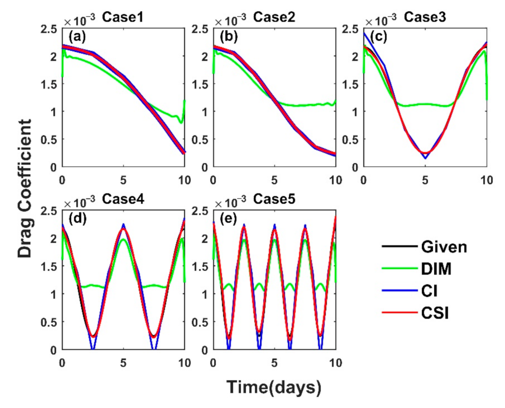
The prescribed and inverted WSDCs are shown in Figure 1. It can be seen that the prescribed distributions of WSDCs (Case 1–5) can be successfully inverted by the CI scheme and the CSI scheme, while they are partially inverted by the DIM scheme. As the distributions become increasingly more complex from Case 3 to Case 5, the consistencies between the inverted distributions obtained by the CI scheme and the prescribed distributions are getting weaker, while the inversions obtained by the CSI scheme are still in good agreement with the prescribed distributions, even at the wave peak and trough.

The mean absolute errors (MAEs) and mean relative errors (MREs) between prescribed and inverted WSDCs after assimilation are shown in

Table 4. The mean absolute error (MAE) and mean relative error (MRE) between the prescribed and inverted WSDCs with different schemes in different cases.

	DIM		CI		CSI
	MAEs	MREs	MAEs	MREs	MAEs	MREs
Case 1	1.79 × 10−4	25.01%	7.89 × 10−6	6.00%	2.77 × 10−6	0.18%
Case 2	3.27 × 10−4	78.25%	7.65 × 10−6	1.07%	3.33 × 10−6	0.61%
Case 3	3.23 × 10−4	76.66%	5.34 × 10−5	5.66%	1.29 × 10−5	1.25%
Case 4	3.62 × 10−4	80.45%	9.78 × 10−5	17.73%	3.34 × 10−5	4.48%
Case 5	3.43 × 10−4	79.25%	1.06 × 10−4	20.00%	3.83 × 10−5	6.34%

. The magnitude orders of MAEs for the DIM scheme were all 10⁻⁴, while those for the CI scheme and CSI scheme were about 10⁻⁵–10⁻⁶. In Case 1, the MRE for the DIM scheme was slightly larger than 25%, and furthermore, the MREs of Case 2–5 were more than 70%, indicating that the results of the DIM scheme were poor. When the distributions were relatively simple (Case 1–3), the MREs of the CI scheme and CSI scheme were less than 6%. Thus, the reliability of the inversion results was high. In addition, the MREs of the CI scheme increased to 17.73% and 20.00% for the two complex distributions (Case 4–5), but the MREs using the CSI scheme remained at a low level (4.48% and 6.34%), which shows that the inversion results of the CSI scheme were more reliable.

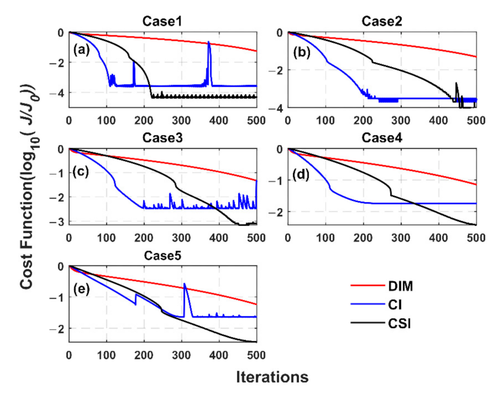
We further analyzed the curves of the normalized cost function, which are shown in Figure 2. It is shown that the cost functions for the DIM scheme were only decreased by 1–2 orders of magnitude. On the contrary, those with the CI scheme and CSI were scheme generally decreased by 2–4 orders of magnitude. The results indicate that the latter two schemes can achieve better simulation results, demonstrating better inverted WSDCs. Although the cost functions of the CSI scheme decreased more slowly than those of the CI scheme during the several early iterations, they were lower after a certain amount of iterations, indicating that the inversion effect of the CSI scheme was more advantageous.

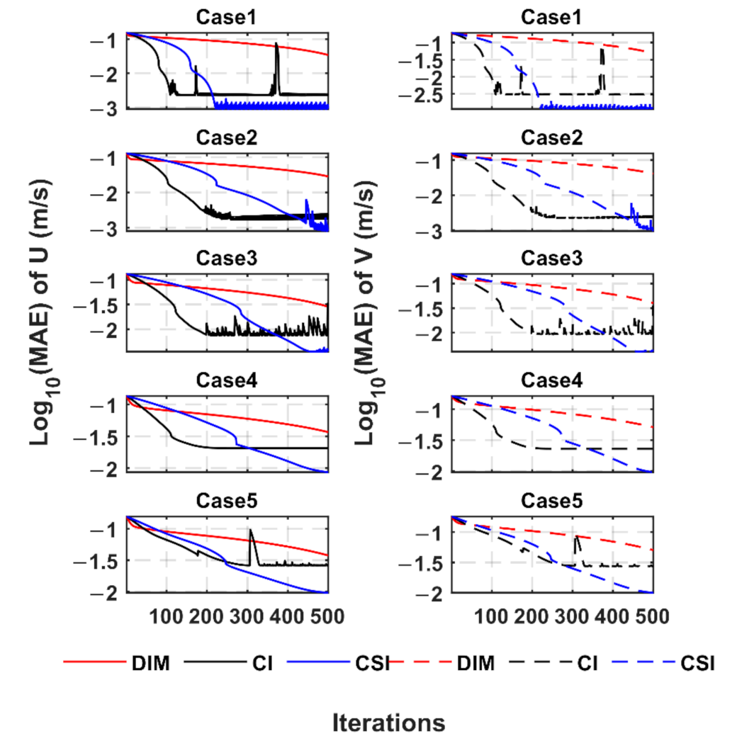
The above results indicate that the CSI scheme showed good inversion ability for WSDCs of different complexities. Here, the simulation ability of current velocity was also assessed. The variations of the MAEs of the horizontal current velocity components (u and v) with the iterations are shown in Figure 3. It can be seen that the MAEs of the CI scheme and the CSI scheme in Cases 1–5 were obviously smaller than those of the DIM scheme. In cases 1–3, the MAEs of the CI scheme decreased more rapidly with increased iteration steps, but the final values of the MAEs were at the same level as those of the CSI scheme. However, for the relatively complex distributions (cases 4–5), the MAEs of the CSI scheme were still smaller than those of the CI scheme.

In conclusion, the prescribed distributions of WSDCs can successfully be inverted by the adjoint method with CI or CSI schemes even if only two layers of data are assimilated. As the WSDCs from Case 1 to Case 5 were increasingly more complex, the CSI scheme obtained the best inversion result, and the CI scheme followed. At the same time, the DIM scheme obtained the worst inversion, again indicating that the IP scheme is an effective tool in parameter estimation based on the adjoint method.

3.2. Estimation of WSDCs under Different Observation Noise

In all the above cases, the perfect observations without any noise were directly produced by the forward model. However, there was noise in the actual observations of current velocity and wind speed, which might have affected the inversion results. Zhang and Lu [35] indicated that the average difference between the inversion results and true values would increase abnormally, so long as observation errors increased to a certain level. Therefore, we designed another group of experiments to investigate the potential effect of different data noise on WSDC estimation. Considering the distribution complexity, the WSDC in Case 5 was adopted in this group. Gaussian white noise was added to observations of current velocity $u(i,j)$, $v(i,j)$ and wind speed $u_a(i)$, respectively, representing the observation errors in the real ocean. Specifically, errors with different ratios to each observation value were added to the perfect observations (shown in

Table 5. The experiment setting in the second group of experiments.

		Noise
Group 2	Case 5–1	3%
	Case 5–2	5%
	Case 5–3	10%
	Case 5–4	15%

). Since group 1 showed that the CI and the CSI schemes were significantly better than the DIM scheme, the former two schemes were used in this group.

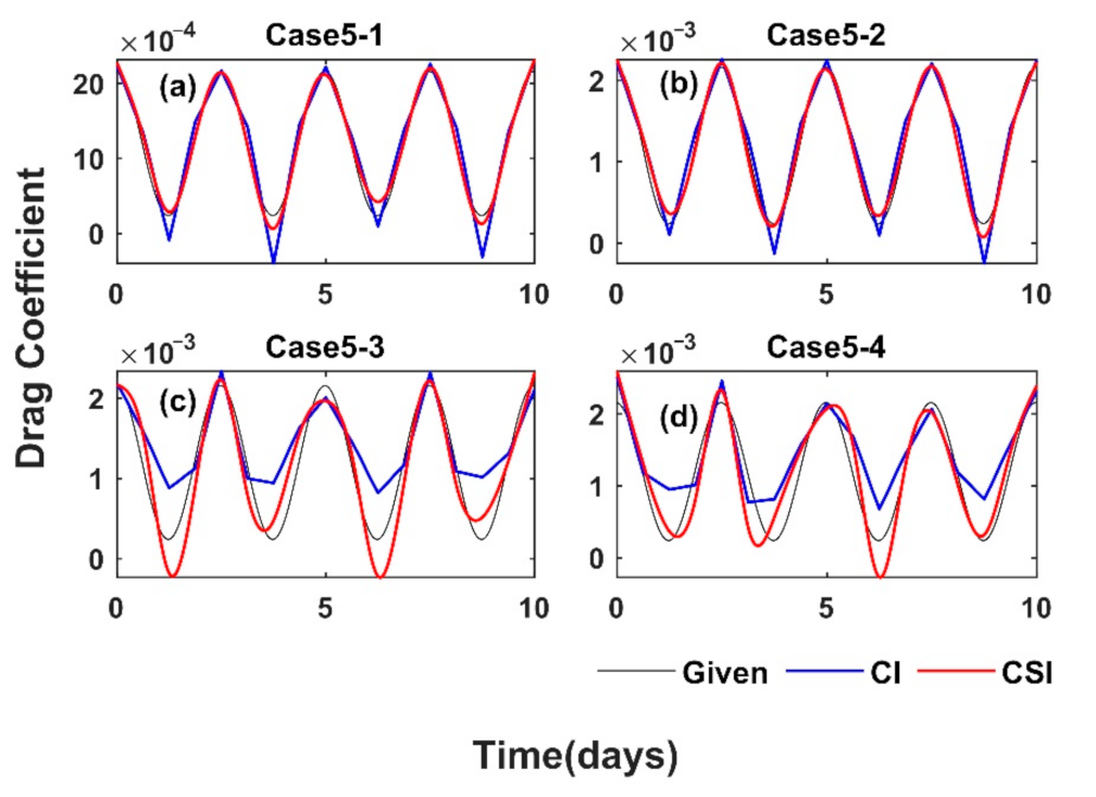
The prescribed and inverted WSDCs for different observation noise are shown in Figure 4, and the correlation coefficients between them are shown in

Table 6. The correlation coefficients between the prescribed and inverted WSDCs with different schemes in different cases.

Scheme	CI	CSI
Case 5–1	0.9741	0.9935
Case 5–2	0.9801	0.9936
Case 5–3	0.9212	0.9402
Case 5–4	0.9152	0.9287

. It is clear that the prescribed distributions could be inverted successfully by the CI and CSI schemes in Case 5–1 and Case 5–2. However, in Case 5–3 and Case 5–4, the curves inverted with the CI scheme oscillated more violently than those with the CSI scheme, indicating that the inversion accuracy of the CSI scheme was higher than that of the CI scheme. Combining these results with Figure 4 and Table 6, it could be found that the CSI scheme was more advantageous, especially in Case 5–3 and Case 5–4. Moreover, the distortions of both schemes began to increase significantly with increasing noise level.

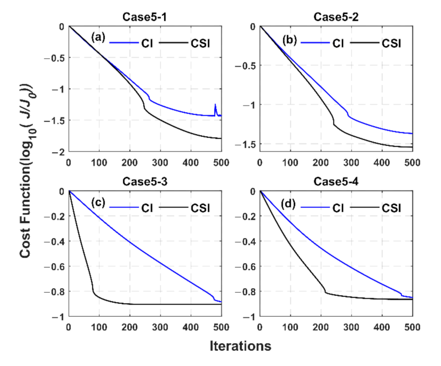
Additionally, it can be found in Figure 5 that the normalized cost functions decline greatly with the iterations. Specifically, at most iterations, the cost functions of the CSI scheme are smaller than those of the CI scheme, indicating that the current velocities simulated by the CSI scheme are closer to the observation. This further reveals the superiority of the CSI scheme.

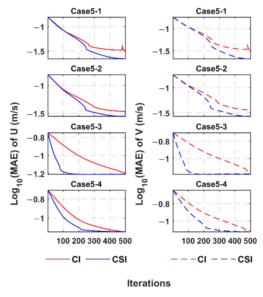
Additionally, the MAEs for the horizontal velocity are shown in Figure 6. It can be seen that, after 200 iterations, the MAEs of the CSI scheme in Case 5-1 were notably smaller than those of the CSI scheme, suggesting that the CSI scheme was more advantageous than the CI scheme.

To sum up, the prescribed distributions of the WSDCs could still be well inverted by the CSI scheme even there were moderate noises in the observations. With the increase in observation errors, the performance of the CSI scheme became worse. Still, the CSI scheme showed a more stable tolerance of observation noise than the CI scheme.

4. Practical Experiments and Results

The twin experiments proved that WSDC can be inverted successfully by the adjoint method and that the CSI scheme is an advantageous scheme compared with other two schemes. However, its performance still needs to be testified with real observation data. To that end, this section conducted practical experiments to invert the WSDCs with the CSI scheme.

4.1. Data and Experimental Design

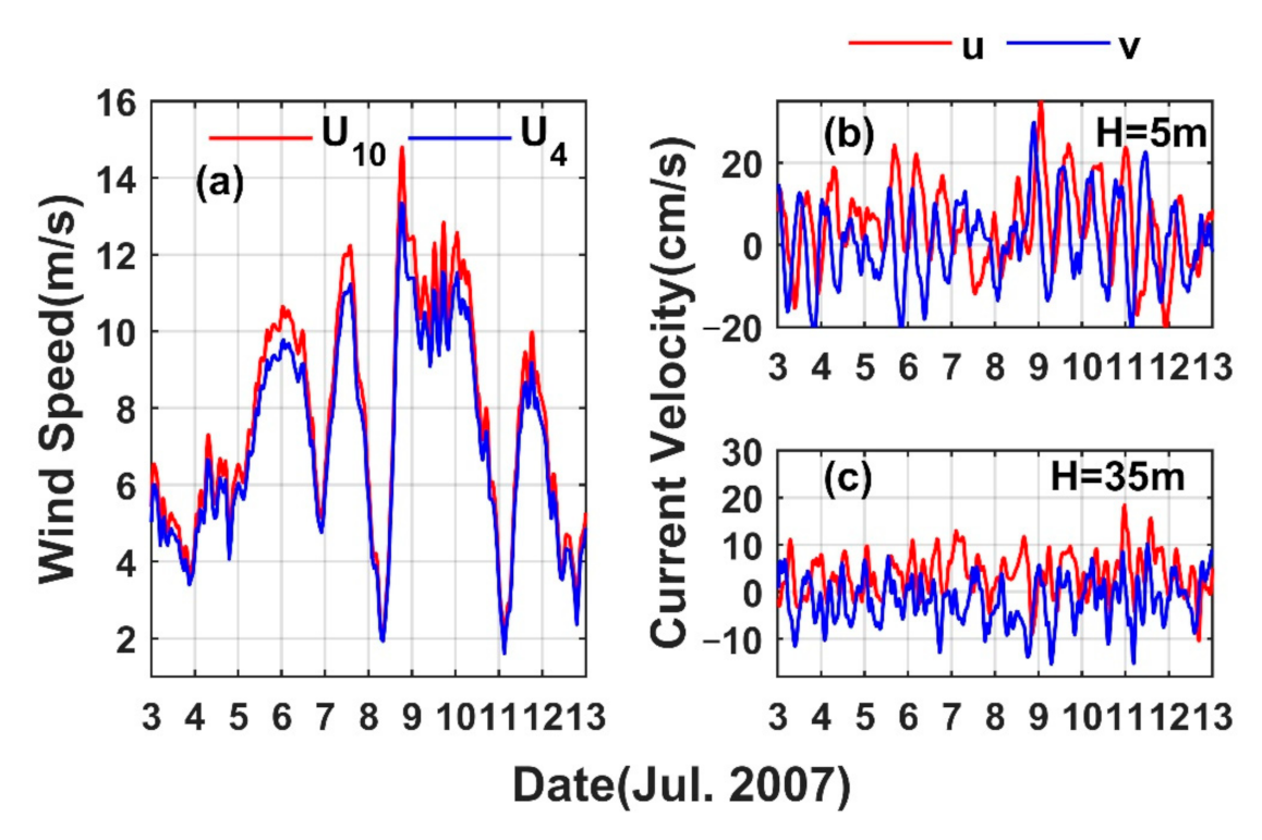
Current velocity and wind speed data were obtained from the ocean mooring station (Papa, 50.1° N,144.9° W) in the mooring system of the Ocean Climate Station Project (OCS) of NOAA, which has been instrumented with upper ocean and surface sensors since June 2007. The current velocity data were measured by an acoustic Doppler current profiler at 5 m and 35 m below the sea surface. The wind speed at an altitude of 4 m measured by the anemorumbometer located at the buoy tower of the sea surface was the average value per hour.

The current velocity and wind speed data of 10 days from 0:00 on 3 July 2007 to 0:00 on 13 July 2007 were selected. As the wind speed was measured at 4 m above the sea surface, it needed to be transformed to the value at 10 m (U₁₀ for short) by a bulk formula [36,37]. The time resolution was transformed from 1 h to 0.5 h by interpolation to meet the demands of the model. The original wind speed (U₄ for short) and U₁₀ are shown in Figure 7a. The time series of current velocity are given in Figure 7b,c.

Considering the significant influence of the number of IPs on inversion results, the IP numbers were set at 21, 41, and 97 (i.e., the intervals of 12 h, 6 h, and 2.5 h, respectively), and the corresponding numerical experiments were named as Cases 6–8, respectively, as shown in

Table 7. The experimental setting in the practical experiments.

	IPs
Case 6	21
Case 7	41
Case 8	97

. The other parameters were set the same as in the twin experiments. Although there was a gap between the zero initial conditions and the real scenarios, the model simulations were gradually adjusted towards the real scenarios by assimilating the observations made.

4.2. Results Analysis

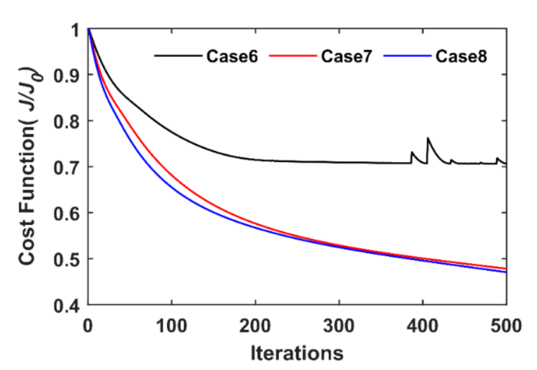
The normalized cost function is shown in Figure 8. After assimilation, the cost function in Case 6 decreased by around 30%, and cost functions in Cases 7–8 decreased significantly by about 50%, which indicates that the CSI scheme is effective in reducing the difference between observed and modeled Ekman velocities. In addition, the parameter optimization effect could be improved by increasing the number of IPs, but not significantly if the number of IPs is further increased.

The MAEs between the inverted and observed velocities could also demonstrate the effectiveness of the CSI scheme, as shown in Figure 9. It could be found that the MAEs in the three cases all showed a declining trend. The MAEs of U (V) in Cases 7–8 were decreased significantly, from 0.065 (0.07) m⋅s⁻¹ to about 0.05 (0.05) m⋅s⁻¹, indicating that the distributions of the WSDCs could be inverted by the CSI scheme competently.

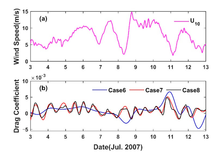
The time-series of WSDCs and standard wind speed (U₁₀) are shown in Figure 10. It was shown that the temporal variation of the WSDCs was closely related to the variations of wind speed. This consistency becomes more obvious with the increasing IPs. The WSDCs had a peak during 7–8 July 2007, which agreed well with the wind speed. After 11 July, the time-varying curve of wind speed had two relatively deep troughs and one sharp peak, and there were similar variations in the distributions of the WSDCs. But there was a certain phase difference between them. This may have been due to defects in the dynamic process of the model and in the observation data, that was available only at 5 m and 35 m depths.

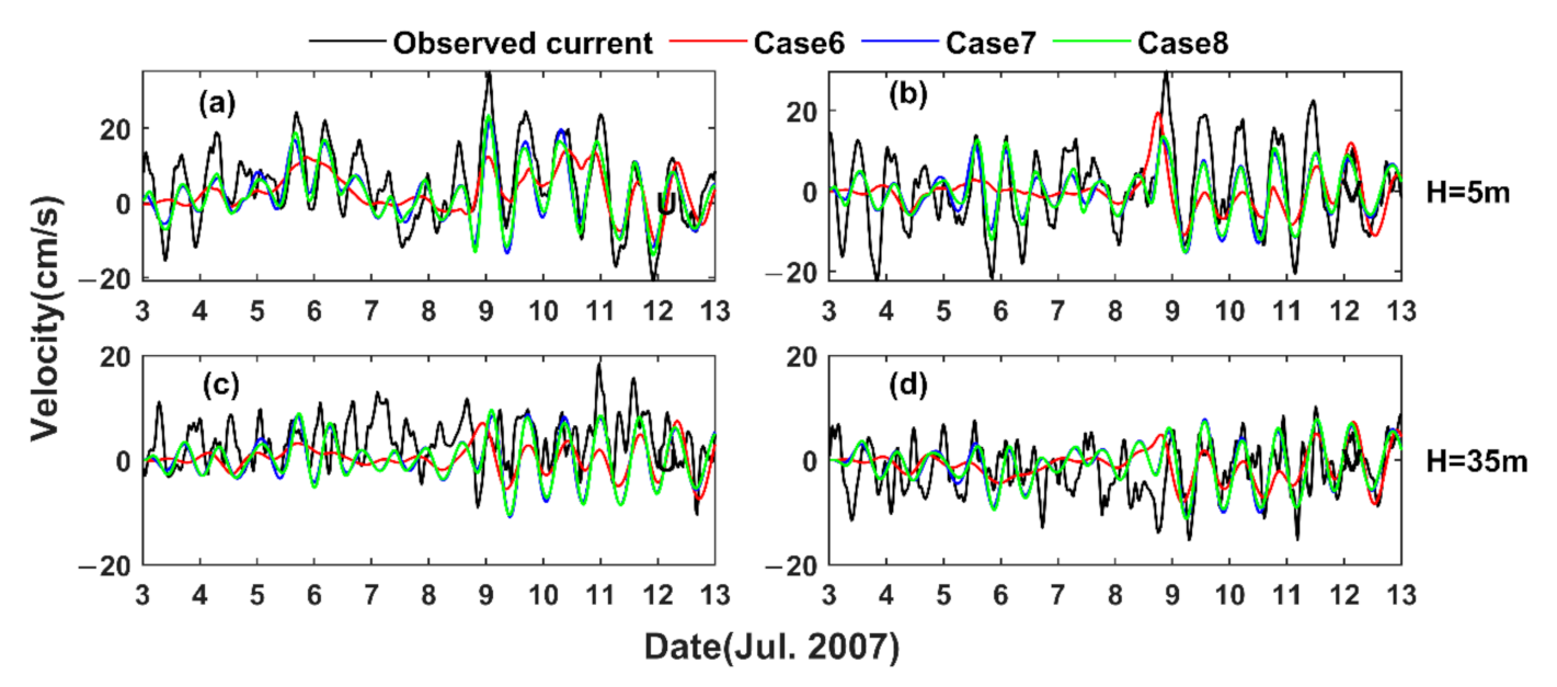
We also compared the time series of observed and inverted current velocities at 5 m and 35 m depth, as shown in Figure 11. For the inverted current velocity at 5 m depth, both the amplitude and phase coincided with observations well, especially in Case 7 and Case 8. However, there were some discrepancies between the modeled results and the observations at 35 m depth. The comparison was also consistent with previous conclusions that the model is more sensitive to upper current velocity.

In summary, the above results had a significant downward trend, indicating that the inverted results were stable. As the IP number increased, the temporal variation of inverted WSDC was more similar to that of wind speed U₁₀. This phenomenon is consistent with physical oceanography in the light of there being a positive correlation between WSDC and wind speed.

5. Conclusions

Based on the adjoint assimilation technique, the CSI scheme was used to invert the time-varying WSDC in the Ekman model. Two groups of twin experiments and one group of practical experiments were carried out. The effectiveness of the CSI scheme was successfully verified by the above experiments. The main conclusions are as follows:

(1)

The first group of experiments showed that the prescribed distributions of WSDCs were successfully inverted by the CI scheme and the CSI scheme, even if only the observations in the first and seventh layers were assimilated—while the prescribed distributions were partially inverted by the DIM scheme. The CSI scheme was more advantageous than the CI and the DIM schemes as the complexity of WSDC increased.

(2)

In the second group, even if there was some noise in the observations, the CSI scheme could invert the distribution of WSDCs successfully. With the observation error increasing, the stability of the CSI scheme was higher than that of the CI scheme, and the results of the CSI scheme were smoother.

(3)

In the practical experiment, the temporal distribution of WSDC inverted by the CSI scheme had a similar variation trend to that of wind speed U₁₀, and a more accurate inverted result could be obtained by the CSI scheme with appropriate IPs.

Overall, this work extends our understanding of the Ekman model and provides an effective method to estimate the time-series of WSDC. However, in the inversion process, some influencing factors are simplified (e.g., the temporal eddy viscosity). Further work, in which the time-varying WSDCs and eddy viscosity are simultaneously estimated, will be the focus.

References

1. Wang, J.; Song, J.; Huang, Y.; Fan, C. On the parameterization of drag coefficient over sea surface. Acta Oceanol. Sin. 2013, 32, 68–74. [Google Scholar] [CrossRef]
2. Chen, S.; Qiao, F.; Jiang, W.; Guo, J.; Dai, D. Impact of Surface Waves on Wind Stress under Low to Moderate Wind Conditions. J. Phys. Oceanogr. 2019, 49, 2017–2028. [Google Scholar] [CrossRef]
3. Smith, S.D.; Anderson, R.J.; Oost, W.A.; Kraan, C.; Maat, N.; De Cosmo, J.; Katsaros, K.B.; Davidson, K.L.; Bumke, K.; Hasse, L.; et al. Sea surface wind stress and drag coefficients: The hexos results. Bound.-Layer Meteorol. 1992, 60, 109–142. [Google Scholar] [CrossRef] [Green Version]
4. Mel, R.A.; Viero, D.P.; Carniello, L.; Defina, A.; D’Alpaos, L. The first operations of Mo.S.E. system to prevent the flooding of Venice: Insights on the hydrodynamics of a regulated lagoon. Estuarine Coast. Shelf Sci. 2021, 261, 107547. [Google Scholar] [CrossRef]
5. Jones, J.; Davies, A. Storm surge computations for the Irish Sea using a three-dimensional numerical model including wave–current interaction. Cont. Shelf Res. 1998, 18, 201–251. [Google Scholar] [CrossRef]
6. Wu, J. Wind-Stress coefficients over Sea surface near Neutral Conditions—A Revisit. J. Phys. Oceanogr. 1980, 10, 727–740. [Google Scholar] [CrossRef] [Green Version]
7. Large, W.G.; Yeager, S.G. The global climatology of an interannually varying air–sea flux data set. Clim. Dyn. 2008, 33, 341–364. [Google Scholar] [CrossRef]
8. Zijlema, M.; van Vledder, G.; Holthuijsen, L. Bottom friction and wind drag for wave models. Coast. Eng. 2012, 65, 19–26. [Google Scholar] [CrossRef]
9. Maurer, K.D.; Bohrer, G.; Kenny, W.T.; Ivanov, V.Y. Large-eddy simulations of surface roughness parameter sensitivity to canopy-structure characteristics. Biogeosciences 2015, 12, 2533–2548. [Google Scholar] [CrossRef] [Green Version]
10. Powell, M.D.; Vickery, P.J.; Reinhold, T.A. Reduced drag coefficient for high wind speeds in tropical cyclones. Nature 2003, 422, 279–283. [Google Scholar] [CrossRef] [PubMed]
11. Hwang, P.A. Temporal and spatial variation of the drag coefficient of a developing sea under steady wind-forcing. J. Geophys. Res. Space Phys. 2005, 110. [Google Scholar] [CrossRef] [Green Version]
12. Kara, A.B.; Wallcraft, A.J.; Metzger, E.J.; Hurlburt, H.E.; Fairall, C. Wind Stress Drag Coefficient over the Global Ocean. J. Clim. 2007, 20, 5856–5864. [Google Scholar] [CrossRef] [Green Version]
13. Edson, J.B.; Jampana, V.; Weller, R.A.; Bigorre, S.P.; Plueddemann, A.J.; Fairall, C.; Miller, S.D.; Mahrt, L.; Vickers, D.; Hersbach, H. On the Exchange of Momentum over the Open Ocean. J. Phys. Oceanogr. 2013, 43, 1589–1610. [Google Scholar] [CrossRef] [Green Version]
14. Pacanowski, R.; Philander, S. Parameterization of Vertical Mixing in Numerical Models of Tropical Oceans. J. Phys. Oceanogr. 1981, 11, 1443–1451. [Google Scholar] [CrossRef]
15. Ferreira, V.G.; Mangiavacchi, N.; Tomé, M.F.; Castelo, A.; Cuminato, J.A.; McKee, S. Numerical simulation of turbulent free surface flow with two-equationk–ɛ eddy-viscosity models. Int. J. Numer. Methods Fluids 2004, 44, 347–375. [Google Scholar] [CrossRef]
16. Mellor, G. Users Guide for a Three-Dimensional, Primitive Equation, Numerical Ocean Model. 2003. Available online: https://www.researchgate.net/publication/242777179_Users_Guide_For_A_Three-Dimensional_Primitive_Equation_Numerical_Ocean_Model (accessed on 1 October 2021).
17. Odier, P.; Chen, J.; Rivera, M.; Ecke, R. Fluid Mixing in Stratified Gravity Currents: The Prandtl Mixing Length. Phys. Rev. Lett. 2009, 102, 134504. [Google Scholar] [CrossRef] [PubMed] [Green Version]
18. Wang, Y.; Qiao, F.; Fang, G.; Wei, Z. Application of wave-induced vertical mixing to the K profile parameterization scheme. J. Geophys. Res. Space Phys. 2010, 115. [Google Scholar] [CrossRef]
19. Zhang, Y.; Tian, J.; Xie, L. Estimation of eddy viscosity on the South China Sea shelf with adjoint assimilation method. Acta Oceanol. Sin. 2009, 28, 9–16. [Google Scholar]
20. Cao, A.-Z.; Chen, H.; Fan, W.; He, H.-L.; Song, J.-B.; Zhang, J.-C. Estimation of Eddy Viscosity Profile in the Bottom Ekman Boundary Layer. J. Atmos. Ocean. Technol. 2017, 34, 2163–2175. [Google Scholar] [CrossRef]
21. Zhang, J.; Li, G.; Yi, J.; Gao, Y.; Cao, A. A Method on Estimating Time-Varying Vertical Eddy Viscosity for an Ekman Layer Model with Data Assimilation. J. Atmos. Ocean. Technol. 2019, 36, 1789–1812. [Google Scholar] [CrossRef] [Green Version]
22. Chen, H.; Cao, A.; Zhang, J.; Miao, C.; Lv, X. Estimation of spatially varying open boundary conditions for a numerical internal tidal model with adjoint method. Math. Comput. Simul. 2014, 97, 14–38. [Google Scholar] [CrossRef]
23. Jiang, D.; Chen, H.; Jin, G.; Lv, X. Estimating Smoothly Varying Open Boundary Conditions for a 3D Internal Tidal Model with an Improved Independent Point Scheme. J. Atmos. Ocean. Technol. 2018, 35, 1299–1311. [Google Scholar] [CrossRef]
24. Pan, H.; Guo, Z.; Lv, X. Inversion of Tidal Open Boundary Conditions of the M2 Constituent in the Bohai and Yellow Seas. J. Atmos. Ocean. Technol. 2017, 34, 1661–1672. [Google Scholar] [CrossRef]
25. Bazilevs, Y.; Hsu, M.; Kiendl, J.; Wüchner, R.; Bletzinger, K. 3D Simulation of Wind Turbine Rotors at Full Scale. Part II: Fluid – Structure Interaction Modeling with Composite Blades. Int. J. Numer. Methods Fluids 2011, 65, 236–253. [Google Scholar] [CrossRef]
26. A Blatov, I.; Dobrobog, N.V.; Kitaeva, E.V. The cubic interpolation spline for functions with boundary layer on a Bakhvalov mesh. J. Phys. Conf. Ser. 2021, 1715, 012001. [Google Scholar] [CrossRef]
27. He, Y.; Li, H.; Wang, S.; Yao, X. Uncertainty analysis of wind power probability density forecasting based on cubic spline interpolation and support vector quantile regression. Neurocomputing 2020, 430, 121–137. [Google Scholar] [CrossRef]
28. Jin, G.; Pan, H.; Zhang, Q.; Lv, X.; Zhao, W.; Gao, Y. Determination of Harmonic Parameters with Temporal Variations: An Enhanced Harmonic Analysis Algorithm and Application to Internal Tidal Currents in the South China Sea. J. Atmos. Ocean. Technol. 2018, 35, 1375–1398. [Google Scholar] [CrossRef]
29. Yu, L.; O’Brien, J.J. Variational Estimation of the Wind Stress Drag Coefficient and the Oceanic Eddy Viscosity Profile. J. Phys. Oceanogr. 1991, 21, 709–719. [Google Scholar] [CrossRef] [Green Version]
30. Zhang, J.; Lu, X. Inversion of three-dimensional tidal currents in marginal seas by assimilating satellite altimetry. Comput. Methods Appl. Mech. Eng. 2010, 199, 3125–3136. [Google Scholar] [CrossRef]
31. Pan, H.; Lv, X.; Wang, Y.; Matte, P.; Chen, H.; Jin, G. Exploration of Tidal-Fluvial Interaction in the Columbia River Estuary Using S_TIDE. J. Geophys. Res. Oceans 2018, 123, 6598–6619. [Google Scholar] [CrossRef]
32. Levi, A.; Sasselov, D.; Podolak, M. The Abundance of Atmospheric CO2in Ocean Exoplanets: A Novel CO2Deposition Mechanism. Astrophys. J. 2017, 838, 24. [Google Scholar] [CrossRef] [Green Version]
33. Sun, W.-Y.; Sun, O.M. Inertia and diurnal oscillations of Ekman layers in atmosphere and ocean. Dyn. Atmos. Oceans 2020, 90, 101144. [Google Scholar] [CrossRef]
34. Zou, Z.; Zhao, D.; Tian, J.; Liu, B.; Huang, J. Drag coefficients derived from ocean current and temperature profiles at high wind speeds. Tellus A: Dyn. Meteorol. Oceanogr. 2018, 70, 1–13. [Google Scholar] [CrossRef] [Green Version]
35. Zhang, J.; Lu, X. Parameter estimation for a three-dimensional numerical barotropic tidal model with adjoint method. Int. J. Numer. Methods Fluids 2007, 57, 47–92. [Google Scholar] [CrossRef]
36. Large, W.G.; Crawford, G.B. Observations and situations of upper-ocean response to wind events during the Ocean Storms Experiment. J. Phys. Oceanogr. 1995, 25, 2831–2852. [Google Scholar] [CrossRef] [Green Version]
37. Zedler, S.E.; Dickey, T.D.; Doney, S.C.; Price, J.F.; Yu, X.; Mellor, G.L. Analyses and simulations of the upper ocean’s response to Hurricane Felix at the Bermuda Testbed Mooring site: 13–23 August 1995. J. Geophys. Res. Space Phys. 2002, 107, 1–29. [Google Scholar] [CrossRef] [Green Version]
Figure 1. The prescribed distributions of WSDCs and inversion distributions of WSDCs obtained by the adjoint assimilation of different schemes. Panels (ae) correspond to Cases 1–5, respectively.
Jmse 09 01220 g001
Figure 2. The variation curves of cost functions with different inversion schemes in Group 1. (ae) correspond to Case 1–Case 5, respectively.
Jmse 09 01220 g002
Figure 3. The MAEs between the observed and inverted velocity components (u and v) in Cases 1–5 (the figure shows the result after taking logarithm log10).
Jmse 09 01220 g003
Figure 4. The prescribed and inverted distributions of WSDCs after adding 3%, 5%, 10%, and 15% errors. Subfigures (a), (b), (c) and (d) represent the addition of 3%, 5%, 10% and 15% errors, respectively.
Jmse 09 01220 g004
Figure 5. The variation curves of cost functions of the CI scheme and the CSI scheme in Group 2. (ad) correspond to Case 5-1–Case 5-4, respectively.
Jmse 09 01220 g005
Figure 6. The MAEs of the horizontal velocity component (u, v) with the assimilation steps after adding 3%, 5%, 10%, and 15% errors (the figure shows the result after taking logarithm log10).
Jmse 09 01220 g006
Figure 7. (a) The time series of the original wind speed U4 and the standard wind speed U10, and the time series of total current velocity u and v for (b) 5 m, and (c) 35 m.
Jmse 09 01220 g007
Figure 8. The cost functions of Cases 6–8.
Jmse 09 01220 g008
Figure 9. The MAEs of the current velocity components (U and V) between inversion results and observations. (a) is U direction, and (b) is V direction.
Jmse 09 01220 g009
Figure 10. Practical experimental results; (a) is the time series distribution of wind speed U10, and (b) is the time series distributions of WSDCs of Case 6–8 using the CSI scheme, respectively.
Jmse 09 01220 g010
Figure 11. The time series of observed and inverted (left) eastward and (right) northward velocity at (a,b) 5 m depth; (c,d) 35 m depth in Cases 6–8.
Jmse 09 01220 g011