
Sand Net Device to Control the Meanders of a Coastal River: The Case of the Authie Estuary (France)


Abstract
:1. Introduction
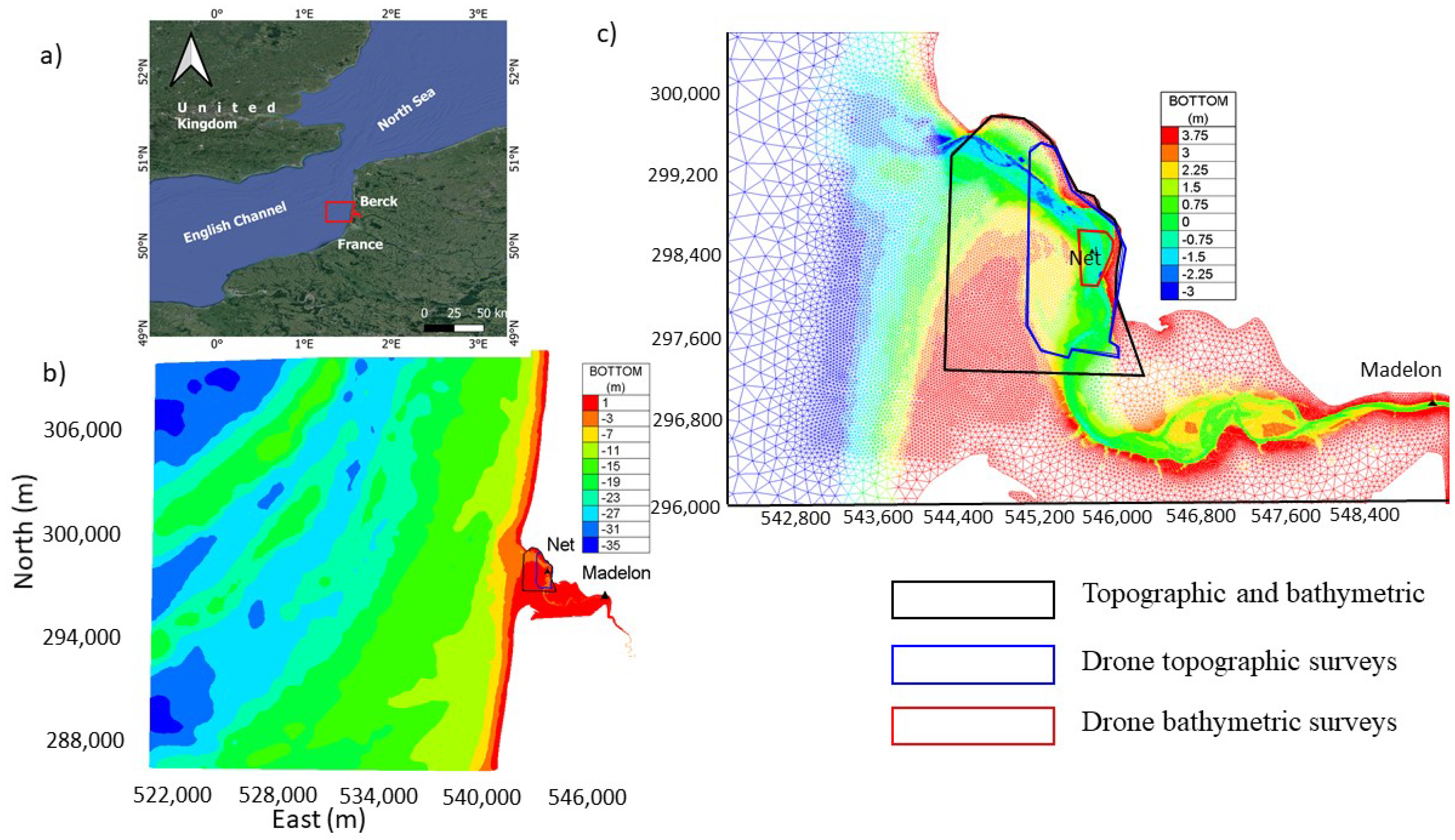
2. Authie Estuary
3. Materials and Methods
3.1. Large Scale Demonstrator of Sand Net Device (SND)
3.2. In Situ Surveys
3.3. Numerical Experiments
3.4. Large-Scale Numerical Model
4. Results and Discussion
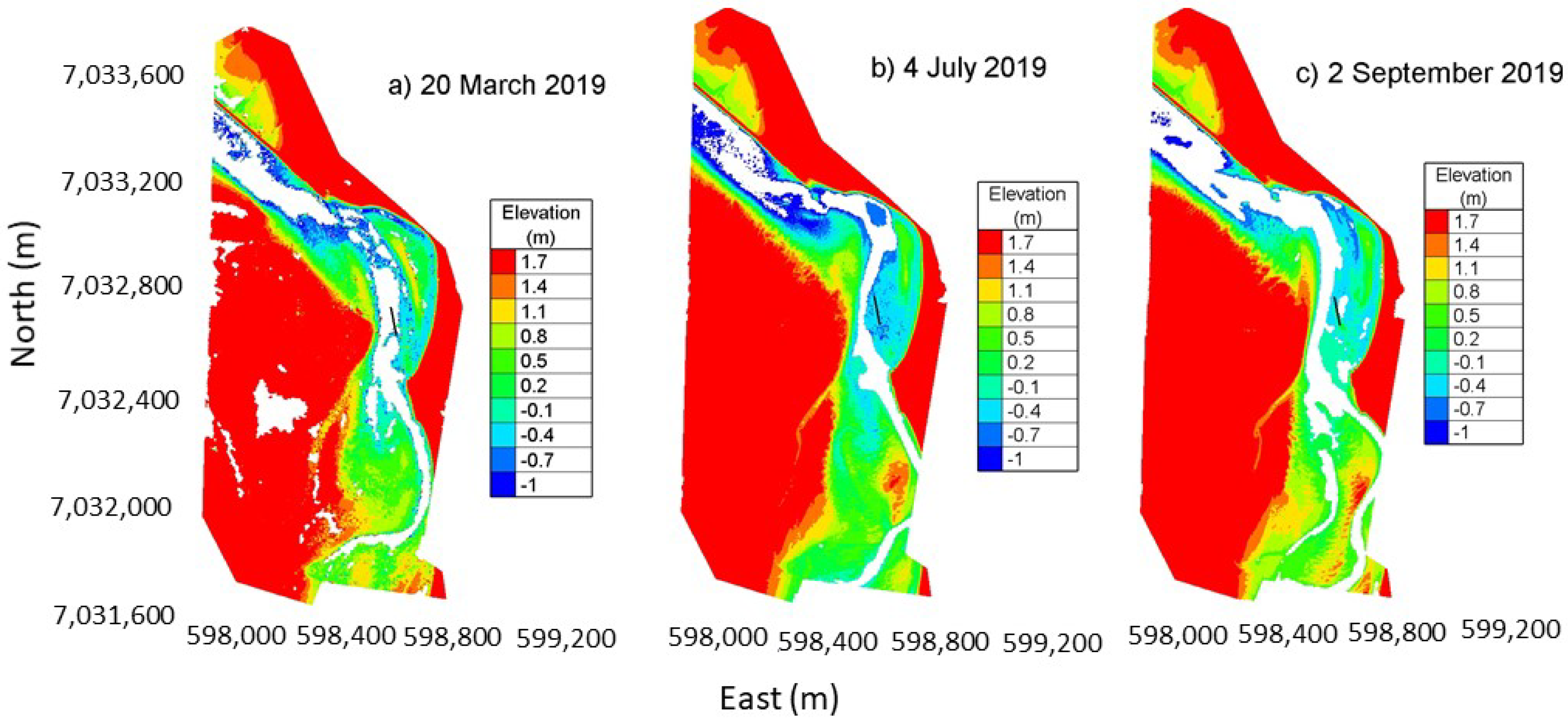
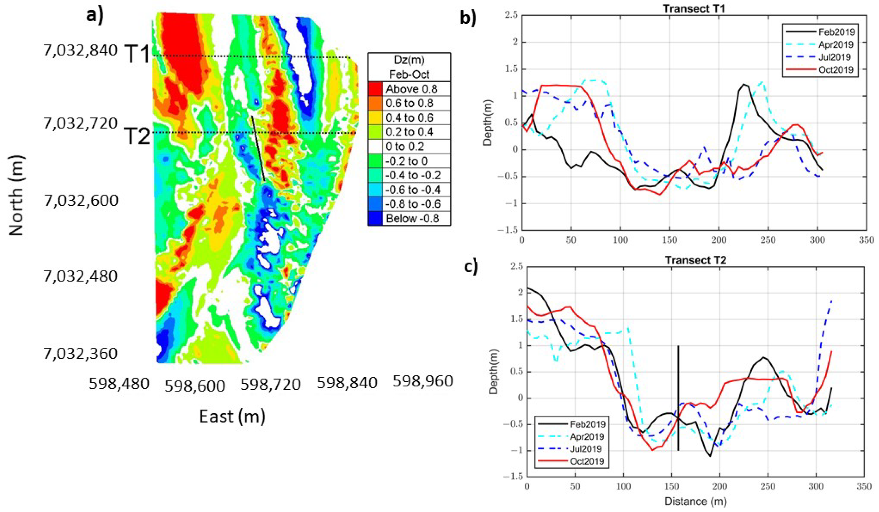
4.1. In Situ Observed Morphodynamic around the SND
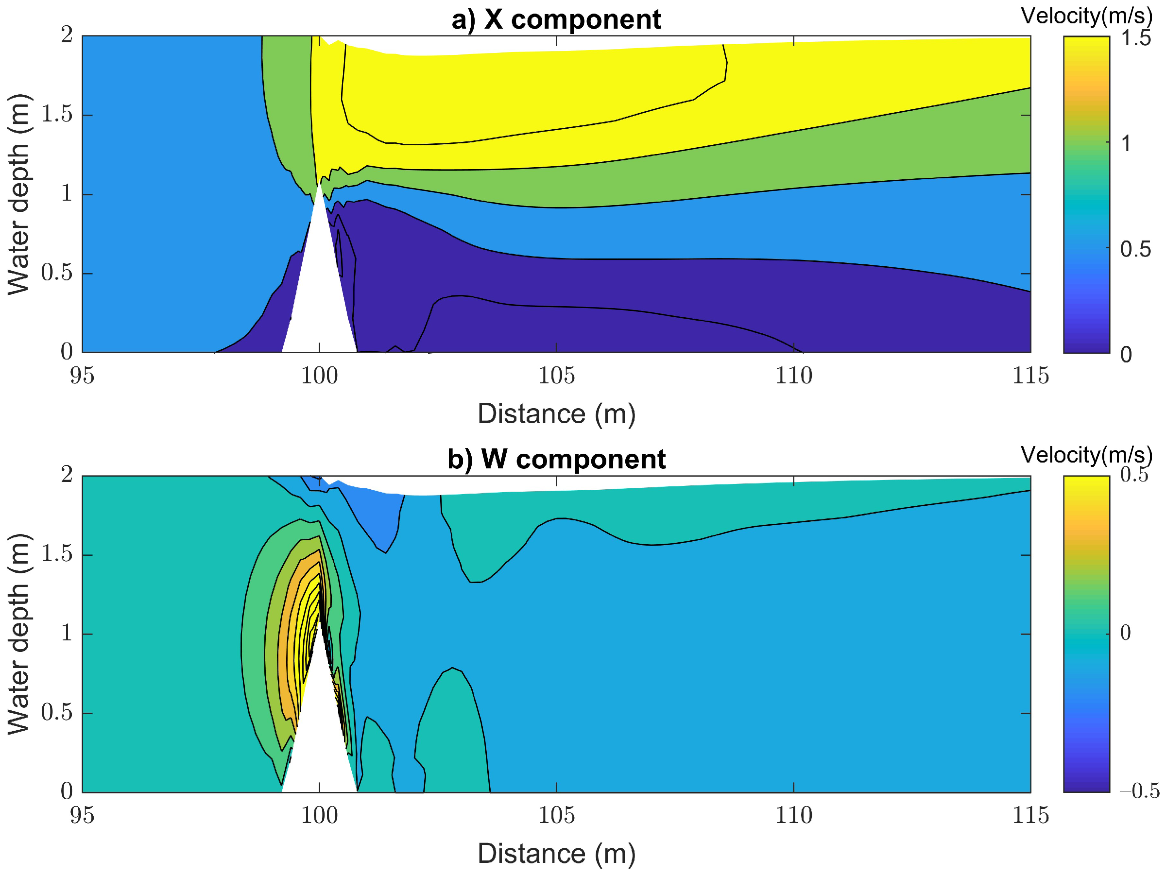
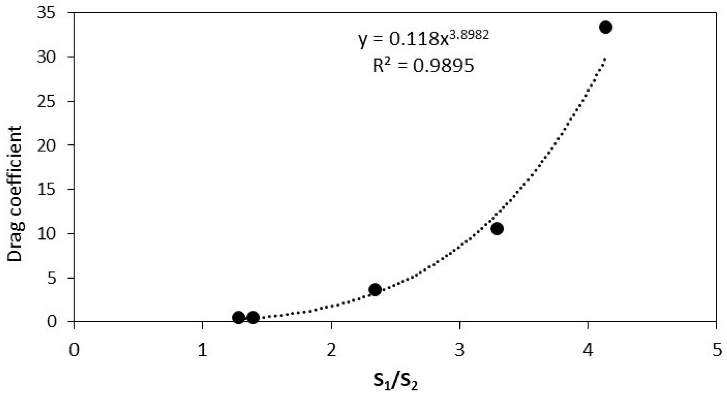
4.2. Estimation of the Drag Coefficient Induced by the SND Using the 3D Numerical Experiments
4.3. Validation of the 2D Hydrodynamic Model
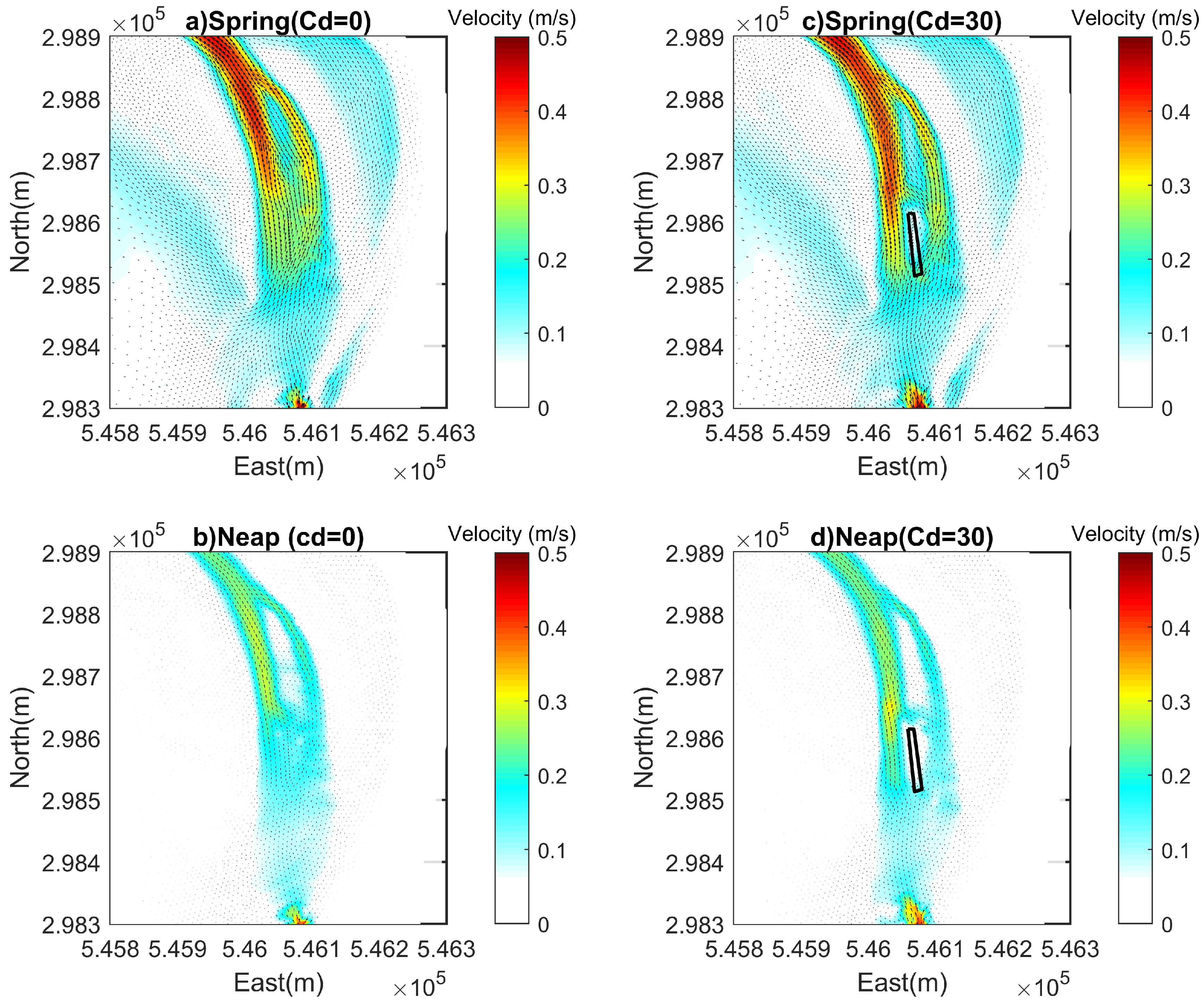
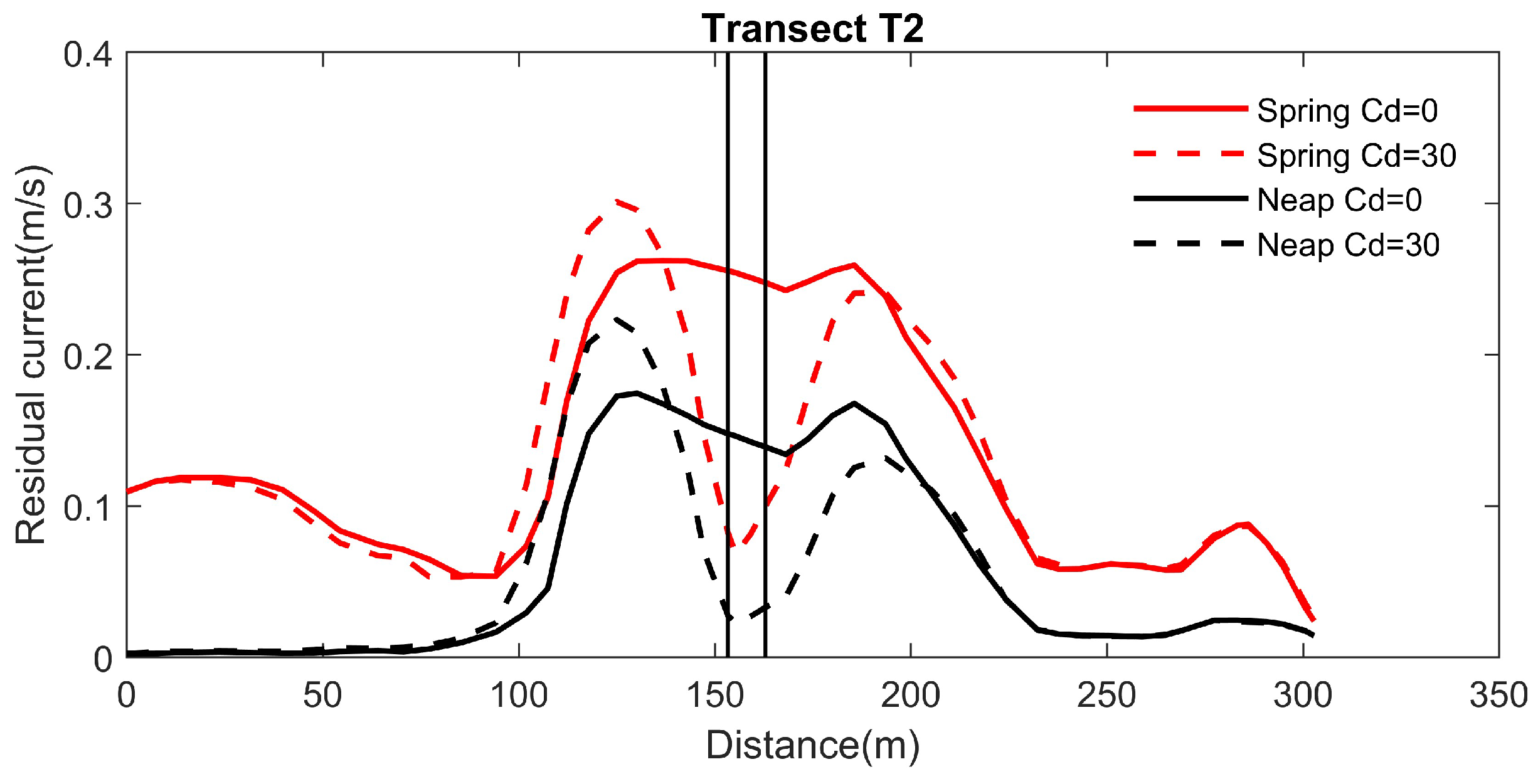
4.4. Influence of the Sand Net on the Residual Current
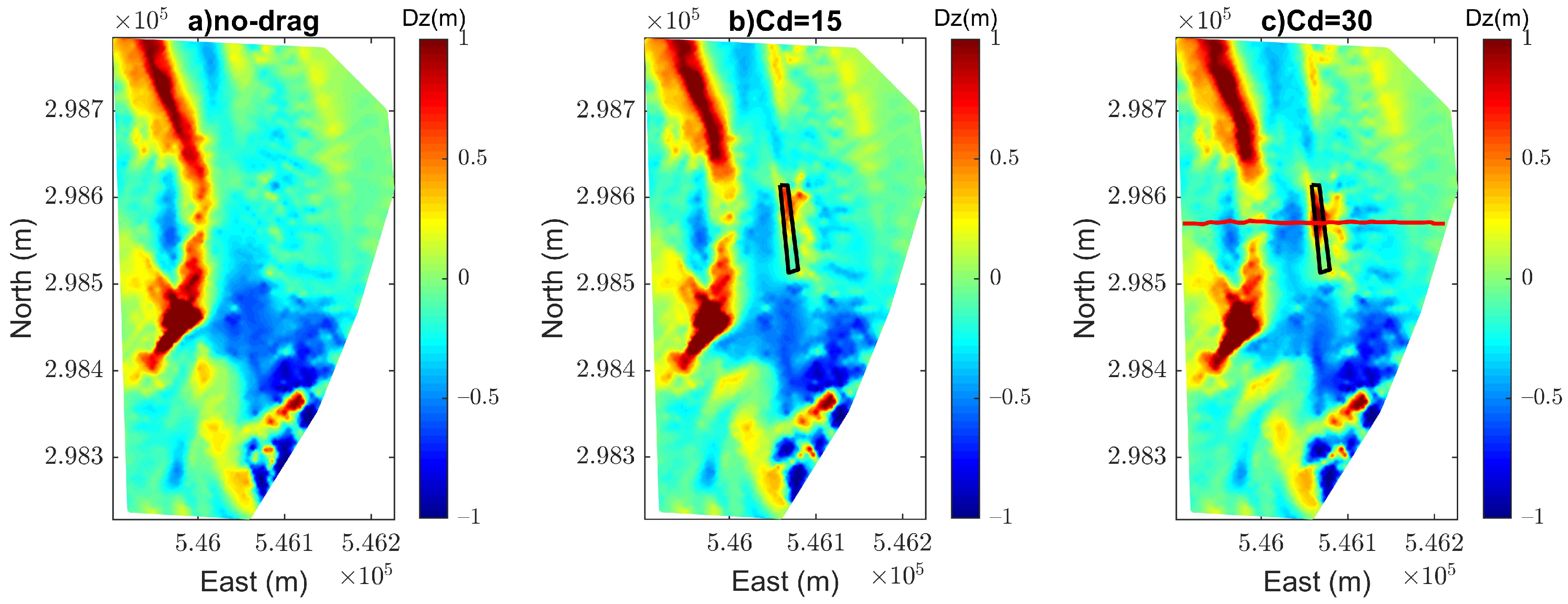
4.5. Influence of Sand Net Installation on Morphodynamics
5. Conclusions
Author Contributions
Funding
Institutional Review Board Statement
Informed Consent Statement
Data Availability Statement
Acknowledgments
Conflicts of Interest
References
- Ridderinkhof, W.; Hoekstra, P.; Van der Vegt, M.; De Swart, H.E. Cyclic behavior of sandy shoals on the ebb-tidal deltas of the Wadden Sea. Cont. Shelf Res. 2016, 115, 14–26. [Google Scholar] [CrossRef]
- Morales, J.A.; Borrego, J.; Jiménez, I.; Monterde, J.; Gil, N. Morphostratigraphy of an ebb-tidal delta system associated with a large spit in the Piedras Estuary mouth (Huelva Coast, Southwestern Spain). Mar. Geol. 2001, 172, 225–241. [Google Scholar] [CrossRef]
- Monge-Ganuzas, M.; Evans, G.; Cearreta, A. Sand-spit accumulations at the mouths of the eastern Cantabrian estuaries: The example of the Oka estuary (Urdaibai Biosphere Reserve). Quat. Int. 2015, 364, 206–216. [Google Scholar] [CrossRef]
- Hesp, P.A.; Ruz, M.H.; Hequette, A.; Marin, D.; Da Silva, G.M. Geomorphology and dynamics of a traveling cuspate foreland, Authie estuary, France. Geomorphology 2016, 254, 104–120. [Google Scholar] [CrossRef]
- Bastos, L.; Bio, A.; Pinho, J.L.S.; Granja, H.; da Silva, A.J. Dynamics of the Douro estuary sand spit before and after breakwater construction. Estuar. Coast. Shelf Sci. 2012, 109, 53–69. [Google Scholar] [CrossRef]
- Sergent, P.; Huybrechts, N.; Smaoui, H. Large Scale Demonstrator of Fishing Nets Against Coastal Erosion of Dunes by Meanders in Authie Estuary (Côte D’Opale—France). In Estuaries and Coastal Zones in Times of Global Change; Springer: Singapore, 2020; pp. 573–593. [Google Scholar]
- Dobroniak, C. Morphological evolution and management proposals in the Authie Estuary, northern France. In Proceedings of the Dunes Estuaries, Koksijde, Belgium, 19–23 September 2015; Volume 2205, pp. 537–545. [Google Scholar]
- Anthony, E.J.; Dobroniak, C. Erosion and recycling of aeolian dunes in a rapidly infilling macrotidal estuary: The Authie, Picardy, northern France. Geol. Soc. Lond. Spec. Publ. 2000, 175, 109–121. [Google Scholar] [CrossRef]
- Dobroniak, C.; Anthony, E.J. Short-term morphological expression of dune sand recycling on a macrotidal, wave-exposed estuarine shoreline. J. Coast. Res. 2002, 36, 240–248. [Google Scholar] [CrossRef]
- Cartier, A.; Héquette, A. Variation in longshore sediment transport under low to moderate conditions on barred macrotidal beaches. J. Coast. Res. 2011, Special Issue 64, 45–49. Available online: http://www.jstor.org/stable/26482130 (accessed on 22 July 2021).
- Marion, C.; Anthony, E.J.; Trentesaux, A. Short-term (≤2 yrs) estuarine mudflat and saltmarsh sedimentation: High-resolution data from ultrasonic altimetery, rod surface-elevation table, and filter traps. Estuar. Coast. Shelf Sci. 2009, 83, 475–484. [Google Scholar] [CrossRef]
- Deloffre, J.; Verney, R.; Lafite, R.; Lesueur, P.; Lesourd, S.; Cundy, A.B. Sedimentation on intertidal mudflats in the lower part of macrotidal estuaries: Sedimentation rhythms and their preservation. Mar. Geol. 2007, 241, 19–32. [Google Scholar] [CrossRef] [Green Version]
- Michon, D. Dispositif et Système de Protection Contre L’érosion du Littoral. EP 2585640 B1, 6 September 2017. [Google Scholar]
- Wang, L.; Shi, Z.H.; Wang, J.; Fang, N.F.; Wu, G.L.; Zhang, H.Y. Rainfall kinetic energy controlling erosion processes and sediment sorting on steep hillslopes: A case study of clay loam soil from the Loess Plateau, China. J. Hydrol. 2014, 512, 168–176. [Google Scholar] [CrossRef]
- Langendoen, E.J.; Mendoza, A.; Abad, J.D.; Tassi, P.; Wang, D.; Ata, R.; El kadi Abderrezzak, K.; Hervouet, J.M. Improved numerical modeling of morphodynamics of rivers with steep banks. Adv. Water Resour. 2016, 93, 4–14. [Google Scholar] [CrossRef] [Green Version]
- Huybrechts, N.; Villaret, C.; Lyard, F. Optimized predictive two-dimensional hydrodynamic model of the Gironde estuary in France. J. Waterw. Port Coast. Ocean. Eng. 2012, 138, 312–322. [Google Scholar] [CrossRef]
- Huybrechts, N.; Villaret, C. Large-scale morphodynamic modelling of the Gironde estuary, France. Proc. Inst. Civ. Eng. Marit. Eng. 2013, 166, 51–62. [Google Scholar] [CrossRef]
- Santoro, P.; Fossati, M.; Tassi, P.; Huybrechts, N.; Van Bang, D.P.; Piedra-Cueva, J.I. A coupled wave–current–sediment transport model for an estuarine system: Application to the Río de la Plata and Montevideo Bay. Appl. Math. Model. 2017, 52, 107–130. [Google Scholar] [CrossRef]
- Tassi, P.; Villaret, C.; Huybrechts, N.; Hervouet, J.M.N. Numerical modelling of 2D and 3D suspended sediment transport in turbulent flows. In Proceedings of the Seventh AIRH Symposium River Coastal an Estuarine Morphodynamics, Beijing, China, 6–8 September 2011. [Google Scholar]
- Hervouet, J.-M. Hydrodynamics of Free Surface Flows: Modelling with the Finite Element Method; John Wiley and Sons Ltd.: West Sussex, UK, 2007; 340p. [Google Scholar]
- Egbert, G.D.; Erofeeva, S.Y. Efficient inverse modeling of barotropic ocean tides. J. Atmos. Ocean. Technol. 2002, 19, 183–204. [Google Scholar] [CrossRef] [Green Version]
- Schureman, P. Manual of Harmonic Analysis and Prediction of Tides; US Government Printing Office: Washington, DC, USA, 1958; Volume 4.
- Audouin, Y.; Benson, T.; Delinares, M.; Fontaine, J.; Glander, B.; Huybrechts, N.; Kopmann, R.; Leroy, A.; Pavan, S.; Pham, C.-T.; et al. Introducing GAIA, the brand new sediment transport module of the TELEMAC-MASCARET system. In Proceedings of the XXVIth TELEMAC-MASCARET User Conference, Toulouse, France, 15–17 October 2019. [Google Scholar]
- Van Rijn, L.C. Unified view of sediment transport by currents and waves. II: Suspended transport. J. Hydraul. Eng. 2007, 133, 668–689. [Google Scholar] [CrossRef]
- Soulsby, R. Dynamics of Marine Sands; Thomas Telford: Telford, London, 1997. [Google Scholar]
- Villaret, C.; Hervouet, J.M.; Kopmann, R.; Merkel, U.; Davies, A.G. Morphodynamic modeling using the Telemac finite-element system. Comput. Geosci. 2013, 53, 105–113. [Google Scholar] [CrossRef]
- Brakenhoff, L.; Schrijvershof, R.; Van Der Werf, J.; Grasmeijer, B.; Ruessink, G.; Van Der Vegt, M. From ripples to large-scale sand transport: The effects of bedform-related roughness on hydrodynamics and sediment transport patterns in delft3d. J. Mar. Sci. Eng. 2020, 8, 892. [Google Scholar] [CrossRef]
- Joly, A.; Pham, C.T.; Andreewsky, M.; Saviot, S.; Fillot, L. Using the DRAGFO subroutine to model Tidal Energy Converters in Telemac-2D. In Telemac User Club 2015; Science and Technology Facilities Council: Warrington, UK, 2015. [Google Scholar]
- Ross, L.; Sottolichio, A.; Huybrechts, N.; Brunet, P. Tidal turbines in the estuarine environment: From identifying optimal location to environmental impact. Renew. Energy 2021, 169, 700–713. [Google Scholar] [CrossRef]
- Crane. Flow of Fluids Through Valves, Fittings, and Pipe; Technical Paper No. 410 th Printing, 197414 th Printing; Crane Ltd.: Ongar, UK, 1974. [Google Scholar]
- Willmott, C.J. On the validation of models. Phys. Geogr. 1981, 2, 184–194. [Google Scholar] [CrossRef]


| Data | Date of Surveys | Area | Data in the Channel of River |
|---|---|---|---|
| Topography and bathymetry | 15 February 2019 | Black line | Yes |
| Topography | 20 March 2019 | Blue line | No |
| Bathymetry | 18 April 2019 | Red line | Yes |
| Topography and bathymetry (Lidar) | 30April 2019 | Whole bay and shoreline | No |
| Topography | 4 July 2019 | Blue line | No |
| Bathymetry | 4 July 2019 | Red line | Yes |
| Topography | 2 September 2019 | Blue line | No |
Publisher’s Note: MDPI stays neutral with regard to jurisdictional claims in published maps and institutional affiliations. |
© 2021 by the authors. Licensee MDPI, Basel, Switzerland. This article is an open access article distributed under the terms and conditions of the Creative Commons Attribution (CC BY) license (https://creativecommons.org/licenses/by/4.0/).
Share and Cite
Do, A.T.K.; Huybrechts, N.; Sergent, P. Sand Net Device to Control the Meanders of a Coastal River: The Case of the Authie Estuary (France). J. Mar. Sci. Eng. 2021, 9, 1325. https://doi.org/10.3390/jmse9121325
Do ATK, Huybrechts N, Sergent P. Sand Net Device to Control the Meanders of a Coastal River: The Case of the Authie Estuary (France). Journal of Marine Science and Engineering. 2021; 9(12):1325. https://doi.org/10.3390/jmse9121325
Chicago/Turabian StyleDo, Anh T. K., Nicolas Huybrechts, and Philippe Sergent. 2021. "Sand Net Device to Control the Meanders of a Coastal River: The Case of the Authie Estuary (France)" Journal of Marine Science and Engineering 9, no. 12: 1325. https://doi.org/10.3390/jmse9121325
APA StyleDo, A. T. K., Huybrechts, N., & Sergent, P. (2021). Sand Net Device to Control the Meanders of a Coastal River: The Case of the Authie Estuary (France). Journal of Marine Science and Engineering, 9(12), 1325. https://doi.org/10.3390/jmse9121325