A Coordination System between Decision Making and Controlling for Autonomous Collision Avoidance of Large Intelligent Ships

Abstract

Large ships are typically with large inertia and longtime delay in motion, in prevailing collision avoidance methods, their maneuverability is generally neglected, there could be a dangerous situation if the system fails to control the ship course as ordered in a timely manner. This paper proposes a coordination system which consists of two algorithms for avoiding risk and then returning to scheduled waypoint. The avoiding risk algorithm are based on VO (velocity obstacle) method, the returning algorithm is derived from LOS (light of sight) guidance. For better performance, the ship model for simulation is a nonlinear Norrbin Model, with the controller improved by CGSA (closed loop gain shaping algorithm) method from traditional PID control, COLREGS (Convention on the International Regulations for Preventing Collisions at Sea) constrains are considered. To test the effectiveness of the proposed system, a series of complex scenarios including Imazu problem are applied.

1. Introduction

Recently, autonomous vehicles have gained a remarkable amount of attention with a focus on solving collision problems by machines [1]. An integrated collision avoidance works following three steps: perceiving, deciding and controlling [2]. However, the deciding and controlling parts are not always working in synchrony, which, as a sequence, may contribute to urgent situations.

In the domain of decision-making technique, research priorities are risk detecting, encounter situation identifying, avoidance algorithm designing etc., problems in this field are generally classified as single and multiple obstacles, or static and dynamic obstacles. A major defect is that the turning orders output by decision-making module are impulsive and generally regardless of how long the control system will complete the order or whether the range of heading turn will cover the constraints of ship maneuverability.

From the perspective of motion control, the key factors are rapidity, stability and robustness to evaluate an autopilot in a process of adjusting the heading angle. Even though significant progress has been made in decades, a ship will never be flexible enough to change heading course instantaneously to expected direction [3].

The inconsistency between decision-making and controlling could result in problems. The decision system gives the ordered course, which is also the desired course according to current status, when the ship turns to the new heading after a period of time, the situation may have changed a lot and the ship may have missed the timing of changing the course, as a sequence the actual trajectory has deviated from the expected. The problem also contributes to a calculation inaccuracy, the DCPA (distance at the closest point of approach) and TCPA (time to the closest point of approach) are more optimistic calculated by a machine mentioned above than the actual data in real time, which may lead to danger of collision or missing the right time to return.

2. Literature Review

Researches [4,5,6] generally applied the ship motion models to simulate the real motion, while the decision and the control part are essentially separated, the maneuverability are ignored. The large inertia and the time lag still have an impact on autonomous navigation.

A number of studies used different ship model to estimate the time delay, model has been utilized to quantify the maneuvering indices by K and T trying to solve the issue. Su [7] calculated the areas a ship needs by the Nomoto [8] model to change its course by 90°. Zhang [9] integrated the differential equations of Nomoto model to obtain the time period for which the rudder comes back to amidships from any angle, the defect is an assumption that the rudder changing is in a moment and the rudder will always return to 0 after maneuvering. the assumptions are generally strict. Wang [10] proposed a numerical method to obtain the latest steering time and minimum course-alteration angle by increasing the time and the course predicted by MMG model, then determining the degree of danger each cycle. The method is effective and simpler than conventional analytical solving.

Heuristic optimization generally sets the motion model as a boundary condition and then obtains the optimum. The method includes genetic algorithm [11], particle swarm optimization [12], ant colony algorithm [13] and neural networking [14], they aimed at the collision avoidance problem by using the advantages of searching ability or nonlinear fitting ability of neuro nets in higher spaces. All the methods mentioned above share the similar idea to find the optimum considering the decision making and controlling as a whole system. The modelled equations of collision avoidance including the maneuverability of ships are usually a nonconvex problem with complex nonlinearity. Strong computation ability is required by these methods, and the initial values are usually random.

Another type of algorithms set up a feasible sections of ship status, they build up databases of decision courses [15,16], control rudders [17] or planning trajectories [18] in respond to different ship status. When the ship is about to act to avoid dangers, the most feasible candidate decision course, control rudder or planning trajectory is selected according to the encounter situations and the status of own ship. The methods actually set up an action dictionary to look up. The difficulty is that the database cannot cover all the cases at sea, especially when the ship is under the influence of circumstances. To solve the problem, Piotr [19] interpolated the unknown data vector based on measurements from turning circle tests, so that the system is able to predict the future state under various initial conditions.

In similar research domains, there are studies focusing on path planning splines [20], arcs [21] or polylines for small unmanned craft to following, the vessel will navigate along the expected routes when it is flexible enough with quality maneuverability, thus the curve planning is more fitting to small robots. Jozef [22] made effective progress on path-planning by game theory, the proposed synthesis can facilitate a mobile robot passing dozens of encounters from other robots. While large ships generally have difficulty in keeping catch of an arbitrary path. controller designing techniques [23,24,25] have also contributed a lot, simulations show satisfied outcomes, while the it generally involves complicated proving processes and numerous parameters to adjust, some of which has no physical meaning, application is a bottle neck.

According to the introduction and literature review above. A coordination system to harmonize the decision and control system is in great need for autonomous collision avoidance on intelligent ships.

The contributions of the paper are as following:

• The risk avoiding algorithm is proposed based on improved VO (velocity obstacle) algorithm by a series of recursive and predictive steps thus the decision-making module will give a more appropriate decision course. The COLREGS (International Regulations for Preventing Collisions at Sea) is also considered.
• The returning waypoint algorithm is proposed based on improved LOS (Line of Sight) method with the predicted ship status. To solve the large crossing problem, an approaching rate is defined to give criterion to identify the problem.
• A more practical controller is applied by CGSA (closed loop gain shaping algorithm) to obtain ship maneuvering time in contrast to traditional ways using simple PID control.
• The collision avoidance and returning functions are combined to a comprehensive system. By shifting among the statuses of avoiding collisions, keeping courses and returning, the own ship will pass the targeted ships outside the boundary of safety domain in a good manner and then return to the next waypoint safely.
• A series of test experiments are conducted including single static obstacle, single targeted ship and multiple targeted ships. The multiple targeted ship encounters are tested based on Imazu problem of 22 cases, then the final two scenarios include up to 7 targeted ships.

3. Modelling of Maneuverability

3.1. Ship Motion Modelling

The main idea in the manuscript is to deal with the lag between the decision making and controlling part, we define that a cargo ship with its length between perpendiculars is longer than 100 m is “large” enough. Another assumption is that the collision avoidance is completed by heading turning. The selection of ship motion model and its parameters should meet these needs.

We used two nonlinear Norrbin models, one is a responding model from rudder to heading for controller designing, the other is a planar motion model for simulation.

The responding model is as following,

$$\ddot{\psi }+\frac{\mathsf{{\rm K}}}{\mathsf{{\rm T}}}H\left(\dot{\psi }\right)=\frac{\mathsf{{\rm K}}}{\mathsf{{\rm T}}}\delta$$

(1)

where, $H\left(\dot{\psi }\right)=\mathsf{\alpha }\dot{\psi }+\mathsf{\beta }{\dot{\psi }}^3$ $\mathsf{\alpha }=8.91$, $\mathsf{\beta }=8467.29$, $\mathsf{{\rm K}}=0.0215$, $\mathsf{{\rm T}}=30.3$, $\mathsf{{\rm K}}$ and $\mathrm{T}$ are the maneuvering indices. For variables $\dot{\psi }=r$ is the angular velocity, $\ddot{\psi }=\dot{r}$ is the angular accelerate, $\delta$ is the rudder.

The nonlinear planar motion model is as follows,

$$\{\begin{array}{c}\dot{u}=a_0\Delta u\\ \dot{v}=a_{11}v+a_{12}r+b_1\delta +F_{Non1}+F_{Wind1}+F_{Wave1}\\ \dot{r}=a_{21}v+a_{22}r+b_2\delta +F_{Non2}+F_{Wind2}+F_{Wave2}\end{array}$$

(2)

where $u$, $v$ and $r$ are surge velocity, sway velocity and yaw rate on ship-attached coordinate. The parameters from $a_0$ to $a_{22}$ as well as $b_1$ and $b_2$ are determined by dimensions of a training ship [26,27], In the equations $F_{Non}, F_{Wind}, F_{Wave}$ are the nonlinear forces and disturbances from wind and wave, the experiment does not involve any circumstances noise, thus the simplified model is as follows:

$$\{\begin{array}{c}\dot{u}=a_0\Delta u\\ \dot{v}=a_{11}v+a_{12}r+b_1\delta +F_{Non1}\\ \dot{r}=a_{21}v+a_{22}r+b_2\delta +F_{Non2}\end{array}$$

(3)

where $F_{Non1}$, $F_{Non2}$ are variables depending on the ship’s sway ($v$) and the rolling ($r$) in real time, the calculation details are from the research by [28].

Small $K_0$ and large $T_0$ indicates that ships are high inertia systems with long time lag for heading changing.

The kinematics formulae (as shown in Equation (3)) transforms the ship motion from the ship-attached to the fixed coordinate system.

$$\{\begin{array}{c}\dot{x}=ucos\psi -vsin\psi \\ \dot{y}=usin\psi +vcos\psi \\ \dot{\psi }=r\end{array}$$

(4)

where $x$ and $y$ define the position on the longitudinal and lateral axis of fixed coordinate, $\psi$ is the heading angle of a ship. Numerical calculations for above differential equations are by the help of fourth order Runge kutta method.

For brief description, we define ${\mathit{X}}_{\mathbf{0}}={\left[x_0,y_0,{\psi }_0,u_0,v_0,r_0,{\delta }_0\right]}^T$ as ship status vector, with the Equations (1)–(4), the updated ship status after some time $t$ is $\mathit{X}={\left[x,y,\psi ,u,v,r,\delta \right]}^T$. The process of predicting ship status by the motion model above could be defined as a function $\mathrm{M}(·)$, the expression is:

$$\mathit{X}=\mathrm{M}\left({\mathit{X}}_{\mathbf{0}},t\right)$$

(5)

If there is a control sequence of rudders $\mathit{u}={\left[{\delta }_{1,}{\delta }_{2,}\dots {\delta }_{t,}\right]}^T$ are input during the time $t$, then the expression is modified as,

$$\mathit{X}=\mathrm{M}\left({\mathit{X}}_{\mathbf{0}},\mathit{u},t\right)$$

(6)

3.2. Autopilot Modelling

There are a number of researches which have made good progress in decision making for collision avoidance of large cargo ships, but for the control system they have only a traditional PID controller with manual tuning. We tried another two methods to design the controller and made a comparison.

Anna [29] applied backstepping approach based on a third order differential equation for ship course keeping. We used the second order model to design a controller because it reduces calculating work while does not lose the feature of time delaying between decision making and control.

Given the state-space equations:

$$\{\begin{array}{c}\dot{x_1}=x_2\\ \dot{x_2}=f\left(x_2\right)+bu\end{array}$$

(7)

where $x_1=\psi$, $x_2=\dot{x_1}=r=\dot{\psi }$, $f\left(x_2\right)=-\left(K/T\right)H\left(\dot{\psi }\right)$, $H\left(\dot{\psi }\right)=\alpha \dot{\psi }+\beta {\dot{\psi }}^3$, $b=K/T$, $u=\delta$ is the rudder angle.

We define ${\psi }_d$ as the desired course, $k_1, k_2\in R^{+}$ as the coefficients for constructing Lyapunov functions, then according to the steps of backstepping method by [30], the controller expression is designed as:

$$u=\frac{T}{K}\left[\frac{K}{T}H\left(x_2\right)-\left(1+k_1{k}_2\right)\left(x_1-{\psi }_d\right)-\left(k_1+k_2\right)\left(x_2-\dot{{\psi }_d}\right)+\ddot{{\psi }_d}\right]$$

(8)

Another method is the CGSA (closed loop gain shaping algorithm) [30], the control law is as follows:

$$\frac{\delta \left(s\right)}{e\left(s\right)}=\left(\frac{1}{K_0{T}_1}+\rho +\frac{T_0}{K_0{T}_1}s\right)\frac{1}{T_{1}s+2}$$

(9)

where the $e\left(s\right)$ denotes the error between current heading and the desired course, $T_1$ is the threshold frequency for controlling, according to the Pierson–Moskowitz spectra [31], the general frequencies of wave disturbance are mainly larger than$0.33\mathrm{rad}/\mathrm{s}$ if the height of the wave are smaller than 7 m, thus to filter the disturbance of wave lower than 7 m, we determine $T_1=10/3$. The only argument to tune is $\rho$, we let $\rho =30$ according to the controlling experiment result. The convergence is proved by [32], the structure of the proposed approach is still a PD-shaped controller, which is feasible for engineering application with better performance.

In guards to rudder limitation, we set a saturation function for the backstepping and CGSA based controllers is used as following:

$$\delta =\{\begin{array}{c}{\mathsf{\delta }}_{\mathrm{L}}, {\delta }_o\ge {\mathsf{\delta }}_{\mathrm{L}} \\ {\delta }_o, -{\mathsf{\delta }}_{\mathrm{L}}\le {\delta }_o\le {\mathsf{\delta }}_{\mathrm{L}}\\ -{\mathsf{\delta }}_{\mathrm{L}}, {\delta }_o\le -{\mathsf{\delta }}_{\mathrm{L}}\end{array} \dot{\delta }=\{\begin{array}{c}{\mathrm{R}}_{\mathrm{L}}, \Delta \delta \ge {\mathrm{R}}_{\mathrm{L}} \\ \Delta \delta , {\mathrm{R}}_L\le \Delta \delta \le {\mathrm{R}}_L\hfill \\ -{\mathrm{R}}_{\mathrm{L}}, \Delta \delta \le -{\mathrm{R}}_L\end{array}$$

(10)

The ${\delta }_o$ is the output of rudder controller, with the limitation ${\mathsf{\delta }}_L=35°$, $\dot{\delta }$ is the rotation speed of rudder engine, we set it within a rational range ${\mathrm{R}}_{\mathrm{L}}=5°/\mathrm{s}$, which indicates that rudder change $\Delta \delta$ will not be quicker than $5°/\mathrm{s}$.

From Figure 1, the backstepping designed controller could well handle the nonlinear problem of the ship model with the shortest adjusting time among the three but a bit of overshoot; the CGSA method are smoother but a little slower. Pure PID fails in control because the added nonlinear terms on the ship model.

From Figure 2, the Backstepping designed controller has a more aggressive control strategy than the CGSA designed controller does, and the PID controller is not applicable because its rudder angle is beyond the limitation of a ship’s range.

This comparison indicates the Backstepping method has the advantage of rapidity while the CGSA method is with a better controlling manner with smaller rudder angle. Given the maneuvering practices that small rudder angle does less harm to the rudder device and consume less power, we finally selected the CGSA designed controller.

The adjusting time of controlling is not easy to obtain, according to transfer functions, we can only find the satisfied predicted results by the ship motion model in Section 3.1, if the allowable error is denoted by 10%, then the adjusting time will be formulated as:

$$\tau =\min \left(\mathrm{t}\right|\left|\right|\psi \left(t\right)-{\psi }_d\left|\right|\le 10\%)$$

(11)

where $\tau$ is the controlling time or adjusting time, which is obtained by finding the first time point when the error of current heading to desired course ${\psi }_d$ is smaller than $10\%$. For brief description in the following parts, the above process of finding controlling time $\tau$ and the rudder control sequence $\mathit{u}={\left[{\delta }_{1,}{\delta }_{2,}\dots {\delta }_{t,}\right]}^T$ are defined as a function $\mathrm{C}(·)$ over desired course ${\psi }_d$ and current own ship status $X_0$.

$${\mathit{C}}_p=\mathrm{C}\left({\psi }_d,{\mathit{X}}_{\mathbf{0}}\right)$$

(12)

where, ${\mathit{C}}_p={\left[\mathit{u},\tau \right]}^T$ are the control parameters.

4. Risk Detection

4.1. Detection Ranges

It is a consensus among researchers that clear area around the ship is mainly important for safe navigation [33], Fujii [34] initially introduced the concept that the safety domain is the area where other ships cannot enter for safety, since then several types of safety domain have been studied for different purposes. Various shapes of areas have been developed in safety domain study [35].

An effective way is to use the time to determine risk of collision, Jinwan [36] proposed an algorithm where the ship will be safe if TCPA is longer than 5 min or the ship has already passed the CPA (Closest Point of Approach) for more than 5 min.

DCPA (distance at the closest point of approach) is another effective way to help with decision making, Shaobo [37] reports that more than 90% of their respondent seafarers will not take any evasive action with a DCPA larger than 1.5 nm. However, the distance will be reduced lower than 1 nm when in congested waters. To adds up the lengths of own and targeted is a simple way but not practical given the maneuverability of ships. Lyu [38] and Sawada [39] used the area with radius of 0.3 nm as the prohibited zone in their collision avoidance experiments, Sawada also took an effort with 0.5 nm but the performance was not as satisfied.

However, the radius of safety domain is obviously not the distance that decision begin to make at. The own ship will detect in advance whether it is in danger of collision with any targeted ship in sight, while it unnecessary to take any action if the targeted ship is far enough, according to rule 22 in COLREGS (International Regulations for Preventing Collisions at Sea), the masthead light in vessels of 50 m or more in length should have an intensity so as to be visible at the minimum range of 6 nm.

Raphael [40] used collision zone, COLREG application zone and free navigation zone in a concentric circle to define areas with different level of risk. Similarly, in this paper, the detection ranges are comprised of two circular areas, as shown in Figure 3, the smaller one around targeted ship is the safety domain with the assumption that ships are bound to collide within the range 0.5 nm. The larger one around own ship is the detection circle where the own ship should take actions to prevent collision if any risk exists, the radius of which is 6.0 nm. thus, a risk parameter is defined as a Boolean value,

$$R=\{\begin{array}{c}1, DCPA\le 0.5 \mathrm{nm}, \mathrm{DIST}<6 \mathrm{nm}\\ 0, DCPA>0.5 \mathrm{nm} \mathrm{or} \mathrm{DIST}<6 \mathrm{nm}\hfill \end{array}$$

(13)

where R = 1 means the danger of collision exists while 0 means safe. DIST is the distance between own ship and the targeted.

4.2. COLREGS Ruling

Basic consensus of actions to avoid collisions is ruled by COLREGS, but without detail positions or directions of encounter situations, which is fundamental at sea for decision making. Tam [41] set up a chart used to determine the encounter types. DING [42] divided all the situation into 12 groups with rights of way. While this is not enough for autonomous collision avoiding, which requires clear choice of starboard or left rudder for a machine to function. The guide of decision under various situations are demonstrated in the diagram Figure 4. The own ship is fixed to head up in the large circle, the sections around it is the bearings from which targeted ships comes. The sections in smaller circle are relative courses with respect to own ship, the colors mean the actions (left or starboard rudder) to take in responding encounter situations. The definitions of different colors and acronyms are explained in

Table 1. Annotation of colors and acronyms.

Color of Areas	Descriptions
	Own ship is in an obligation to give way, the starboard rudder should be taken.
	Own ship should keep course and speed and take necessary actions (starboard or left rudder) when the give-way vessel does not take appropriate actions.
	Own ship is in the overtaking situation, free to take starboard or left rudder but is always on duty of giving way
Acronyms	Encounter Situations
HO	Head on
RC	Right cross
LC	Left Cross
OT1	Overtaking
OT2	Overtaken

.

5. Coordination System

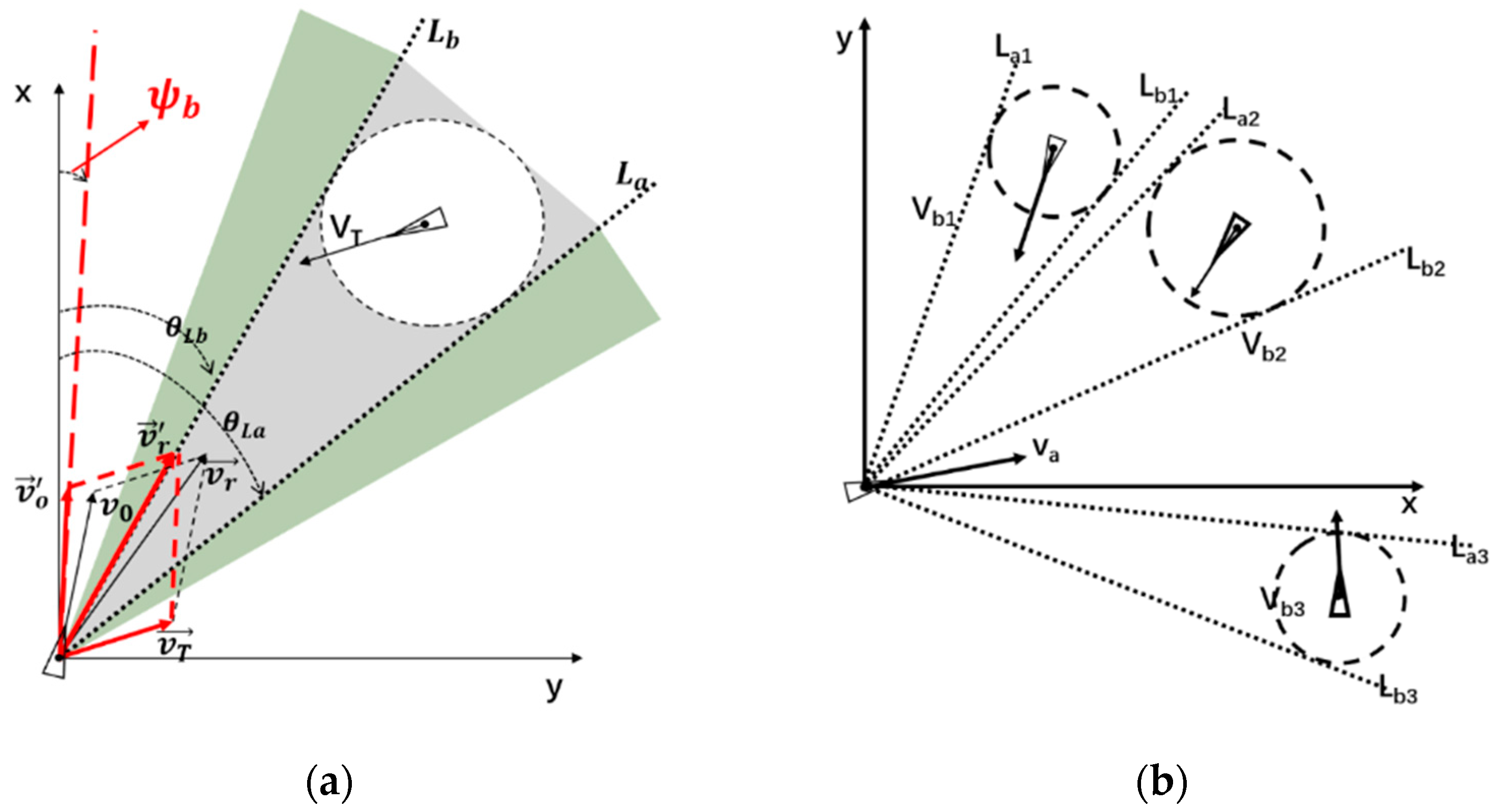
5.1. Basic Principle of VO Algorithm

Many researchers have utilized the velocity obstacle (VO) method to solve avoiding collisions problems [43,44,45]. As is shown in the Figure 5a, ${\mathit{v}}_{\mathbf{0}}$, ${\mathit{v}}_{\mathit{T}}$ are denoted as the velocity vector of own and targeted ship, targeted ships are set on the assumption that they navigate at a constant velocity in this paper. ${\mathit{v}}_{\mathit{r}}={\mathit{v}}_{\mathbf{0}}-{\mathit{v}}_{\mathit{T}}$ is the relative velocity with the included angle ${\theta }_r$, ${\mathrm{L}}_a$ and ${\mathrm{L}}_b$ are the boundaries lines tangent to the safety domain with the angles ${\theta }_{Lb}$ and ${\theta }_{La}$, if ${\theta }_{Lb}$ is chosen as the candidate relative decision course, according to the trigonometric relation, the angle ${\psi }_b$ of ${\mathit{v}}_{\mathit{0}}^{\prime }$ is one of the candidate decision courses of own ship, another result based on ${\theta }_{La}$ is ${\psi }_a$, then the final decision course can be formulated as:

$${\psi }_d=\underset{{\psi }_a or {\psi }_b}{\min }(\Vert {\psi }_0-{\psi }_a\Vert , \Vert {\psi }_0-{\psi }_b\Vert )$$

(14)

Note that the decision course is calculated by simple VO algorithm instead of a final output.

As regard to situations where multiple ships are encountering with own ship. There are a series of boundary courses to each targeted ship, as shown in Figure 5b, we employed a collection of all the candidate decision courses, $\mathrm{CD}=\left\{{\psi }_{\mathrm{a}1},{\psi }_{\mathrm{b}1},{\psi }_{\mathrm{a}2},{\psi }_{\mathrm{b}2},\dots {\psi }_{\mathrm{a}n},{\psi }_{\mathrm{bn}}\right\}$, CD is the acronym of candidate decisions, Then the decision course presents as:

$${\psi }_d=\underset{{\psi }_{an} or {\psi }_{bn}}{\min }(\Vert {\psi }_0-{\psi }_{an}\Vert , \Vert {\psi }_0-{\psi }_{bn}\Vert | n=1,2,3\dots )$$

(15)

Due to minor disturbances of environment, an error correction ${\Delta }_{\psi }$ will be add to the decision course, thus the actual decision course will be:

$${\psi }_d={\psi }_d+{\Delta }_{\psi }$$

(16)

${\Delta }_{\psi }$ is set as $3°$ in this paper.

For brief description in the following parts, the process above to find the decision course based on VO is defined as a function $\mathrm{D}(·)$, thus

$${\psi }_d=\mathrm{V}\left(\mathit{X},{\mathit{X}}_{\mathit{T}}\right)$$

(17)

where the $\mathit{X},{\mathit{X}}_{\mathit{T}}$ are statuses of own and targeted ship.

5.2. Collision Avoiding Algorithm

Due to the maneuverability of ships, the actual trajectory will not always be as expected, the deviation generally varies by ship status and decision course. A practical coordination approach for further modifying the decision course is proposed as followed.

In respond to the ends at each Section 3.2 and Section 5.1, with the Equations (6), (12) and (17), the problem to find the best collision avoidance decision course could be formulated as:

$${\psi }_d=\mathrm{V}\left({\mathit{X}}_{\mathbf{0}},{\mathit{X}}_{\mathit{T}\mathbf{0}}\right)$$

(18)

Which subjects to,

$$\{\begin{array}{c}{\mathit{C}}_p=C\left({\psi }_d,{\mathit{X}}_{\mathbf{0}}\right)\\ \mathit{X}=M\left({\mathit{C}}_p,{\psi }_0\right)\\ {\mathit{X}}_{\mathit{T}}={\mathit{X}}_{\mathit{T}\mathbf{0}}+{\mathit{V}}_{\mathit{T}}t\\ R\left(\mathit{X},{\mathit{X}}_{\mathit{T}}\right)=0\end{array}$$

(19)

The equations comprise of many unknown quantities and nonlinear functions, traditional approaches will involve heavy computation requirements. The proposed collision avoiding steps are demonstrated in the diagram below in Figure 6a, while the flow chart of every single iteration is shown in Figure 6b.

For iteration we define $\mathrm{k}=0,1,2\dots \mathrm{The}\mathrm{appraoch}\mathrm{are}\mathrm{listed}\mathrm{as}\mathrm{following}\mathrm{steps}:$

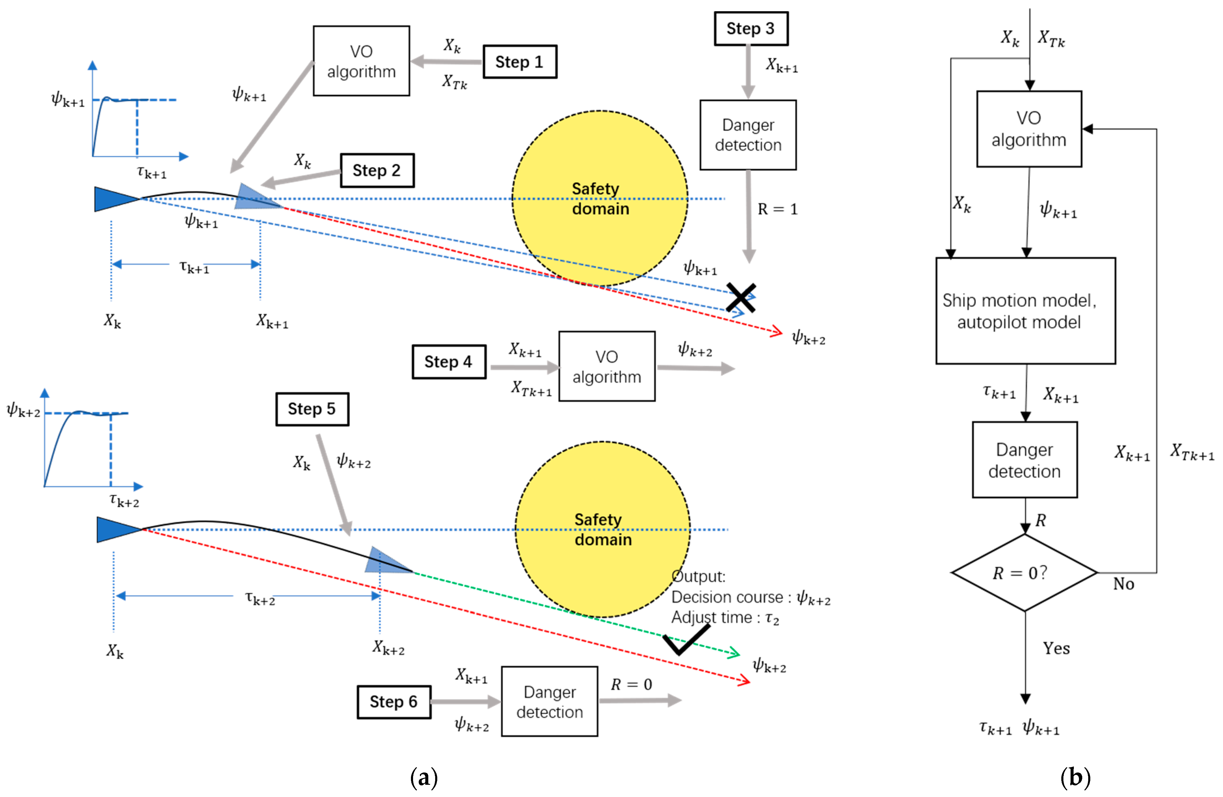
• (Step 1) The simple VO algorithm initially calculates the candidate desired course ${\psi }_{\mathrm{k}+1}$ under current ship status ${\mathit{X}}_{\mathbf{k}}$ and the targeted ship ${\mathit{X}}_{\mathit{T}\mathbf{k}}$.
• (Step 2) The controller and the ship model calculate the control parameters ${\mathit{C}}_{pk+1}={\left[{\mathit{u}}_{\mathbf{k}+\mathbf{1}},{\tau }_{\mathrm{k}+1}\right]}^T$ and predicted own ship status ${\mathit{X}}_{\mathbf{k}+\mathbf{1}}$, ${\mathit{u}}_{\mathbf{k}+\mathbf{1}}={\left[{\delta }_{1,}{\delta }_{2,}\dots {\delta }_{t,}\right]}^T$ is rudder control sequence and ${\tau }_{\mathrm{k}+1}$ is adjusting time of the ship when heading to the desired course ${\psi }_{\mathrm{k}+1}$.
• (Step 3) The danger detection function ($R=1$) indicates that own ship will be in a danger of collision if gets into the predicted status ${\mathit{X}}_{\mathbf{k}+\mathbf{1}}$ by following the desired course ${\psi }_{\mathrm{k}+1}$.
• (Step 4~Step 6) The VO algorithm recalculates a new desired ${\psi }_{\mathrm{k}+2}$ under the predicted own ship status ${\mathit{X}}_{\mathbf{k}+\mathbf{1}}$ and predicted targeted ship ${\mathit{X}}_{\mathit{T}\mathit{k}+\mathbf{1}}$ (assuming that the targeted ship steers in a constant speed), the controller and the ship model, on the bases of ${\psi }_{\mathrm{k}+2}$ and ${\mathit{X}}_{\mathbf{k}+\mathbf{1}}$, will update the adjusting time ${\tau }_{\mathrm{k}+2}$ and predicted own ship status ${\mathit{X}}_{\mathbf{k}+\mathbf{2}}$.
• (Output) According to ${\mathit{X}}_{\mathbf{k}+\mathbf{2}}$ if the value of the detection function turns to R = 0, the final desired course will be ${\psi }_{\mathrm{k}+2}$, the adjust time ${\tau }_{\mathrm{k}+2}$, and the predicted own ship status ${\mathit{X}}_{\mathbf{k}+\mathbf{2}}$, otherwise $R=1$ and the collision avoiding algorithm will repeat the steps 1~3.

Note: The safety domain of the targeted ship is assumed as a circular area, the candidate desired course will update after each iteration by increasing gradually but not larger than $\pm 90°$, the iteration will not stop until there is an appropriate desired course and a safe predicted status ($R=0$) for the own ship. The above procedures will converge in limited time, otherwise the procedures will throw an error indicating that the initial distance to the obstacle is so short that large course changing will not help even with a hard over rudder all the time.

5.3. Returning to Waypoint Algorithm

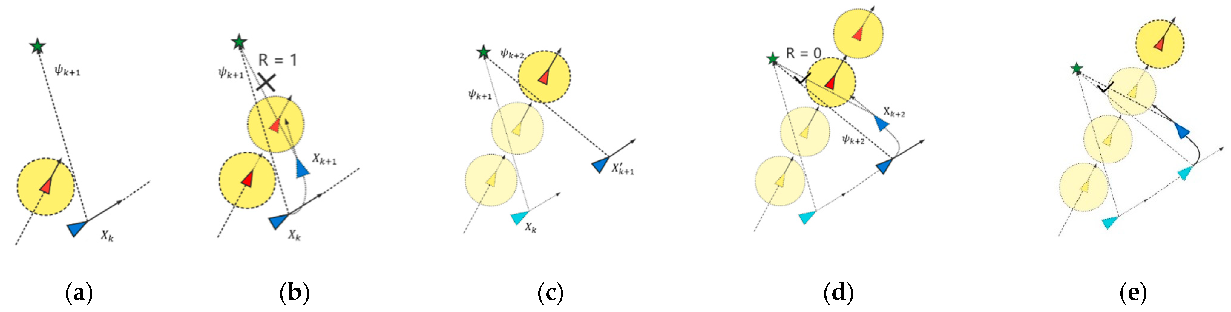
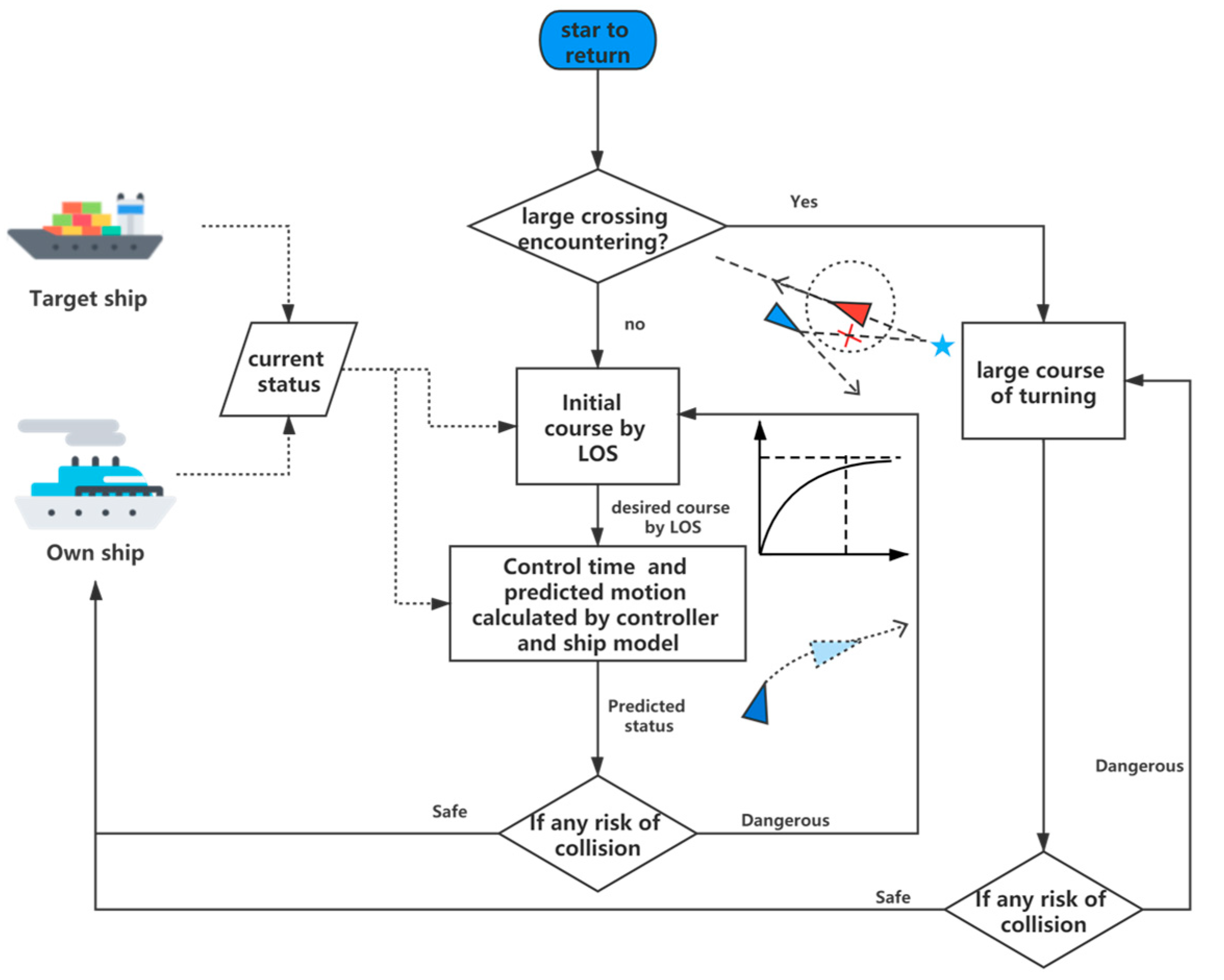
For own ship returning to the scheduled route when the targeted ship is past and the clear, the LOS (light of sight) method is used to determine the desired course for returning. the angle to the next waypoint is the initial desired course ${\psi }_{LOS}$.

The problem is that the ship will not change its course immediately due to its maneuverability and thus may intrude the safety domain of the targeted ship. the method in Section 3.1 for collision are applied, the returning problem expression can be obtained as to find the feasible desired course ${\psi }_{LOS}$.

$${\psi }_{LOS}=\mathrm{L}\left({\mathit{X}}_0,{\mathit{X}}_{\mathit{w}}\right)$$

(20)

Subject to,

$$\{\begin{array}{c}{\mathit{C}}_p=C\left({\psi }_{LOS},{\mathit{X}}_{\mathbf{0}}\right)\\ \mathit{X}={\rm M}\left({\mathit{C}}_p,{\psi }_{LOS}\right)\\ {\mathit{X}}_{\mathit{T}}={\mathit{X}}_{\mathit{T}\mathbf{0}}+{\mathit{V}}_{\mathit{T}}t\hfill \\ R\left(\mathit{X},{\mathit{X}}_{\mathit{w}},{\mathit{X}}_{\mathit{T}}\right)=0\end{array}$$

(21)

The process of finding desired course ${\psi }_{LOS}$ based on LOS method is defined as a function of $\mathrm{L}\left({\mathit{X}}_{\mathbf{0}},{\mathit{X}}_{\mathit{w}}\right)$, Where the ${\mathit{X}}_{\mathbf{0}}$ is the current status of own ship, ${\mathit{X}}_{\mathit{w}}$ is the position of the waypoint. $\mathsf{{\rm M}}\left({\mathit{C}}_p,{\psi }_{LOS}\right)$ is the ship model function predicting the future status${\rm X}$ of own ship with the control variables ${\mathit{C}}_p={\left[\mathit{u},t\right]}^T$ calculated by the controller function $\mathrm{C}\left({\psi }_{LOS},{\mathit{X}}_{\mathbf{0}}\right)$, $\mathit{u}={\left[{\delta }_{1,}{\delta }_{2,}\dots {\delta }_{t,}\right]}^T$ is the rudder sequences during the controlling time $t$ (also called adjust time).${\mathit{X}}_{\mathit{T}}$ is the predicted position of targeted ship from its initial status ${\mathit{X}}_{\mathit{T}\mathbf{0}}$ and velocity ${\mathit{V}}_{\mathit{T}}$. The risk detection function will verify if the predicted $\mathit{X},{\mathit{X}}_{\mathit{w}} \mathrm{and} {\mathit{X}}_{\mathit{T}}$ are in safe (R = 0) or not (R = 1).

As shown in the diagram (Figure 7), the algorithm steps are as follows:

• The returning desired course ${\psi }_{\mathrm{k}+1}$ is generated by LOS method (in the Figure 7a).
• The ship model as well as the controller model calculate the predicted status${\mathit{X}}_{\mathbf{k}+\mathbf{1}}$ of own ship and the targeted ship based on initial status ${\mathit{X}}_{\mathbf{k}}$ (in the Figure 7b).
• The detection function finds that $R=1$ based on predicted status, indicating that a collision accident is about to happen if the desired course ${\psi }_{K+1}$ is followed (in the Figure 7b). The own ship then keeps on its initial course not returning to the way point for an interval. (in the Figure 7b,c), after that interval the own ship repeats Step 1~2 with the current status $X_{k+1}^{\prime }$, and then check the value of R this time, if it indicates safety, the own ship will return following the desired course ${\psi }_{\mathrm{k}+2}$ (in the Figure 7d–e).

The procedures above prevent the own ship from returning to the scheduled route when it is not safe and let the own ship keep its initial course waiting for next attempt, the waiting time is equal to the cycling interval of the whole collision avoidance system. The iteration will not stop until it finds the appropriate desired course ($R=0$) to follow. The flowchart of each iteration is illustrated in Figure 8.

5.4. Large Angle Crossing Problem

Due to the characteristics of the VO algorithm and the returning algorithm, an obvious defect exists that when the encountering ships are in a situation of large angle crossing with similar velocity on the beam of the own ship, the own ship will not return to the next waypoint for quite a long time. As shown in Figure 9 the two ships are almost parallel with no risk of collision, the VO algorithm will not function, but it is difficult for the own ship to return to the waypoint, the returning algorithm in will stop own ship’s each attempt to return because when the ship changes its heading a small DCPA will generate. The own ship will keep its course for very long time until its LOS course is free out of the safety domain. General practice in navigation is to change course to the other side of the targeted ship with a large angle as is shown in the Figure 9.

We proposed a method to identify the situation and let the ship change its course to the other side sharply enough for returning.

As shown in the Figure 10, where $\mathrm{D}$ is the distance between own and targeted ship, ${\mathit{v}}_{\mathit{o}}$, ${\mathit{v}}_{\mathit{T}}$ are velocities of own and targeted ship, ${\mathit{v}}_{\mathit{r}}={\mathit{v}}_{\mathit{o}}-{\mathit{v}}_{\mathit{T}}$ is the relative velocity with respect to targeted ship, ${\theta }_{\mathrm{r}}$ is the angle of ${\mathit{v}}_{\mathit{r}}$, ${\theta }_{\mathrm{b}}$ is the bearing angle, ${\mathit{v}}_{\mathit{d}}$ is the projection on $\mathrm{D}$ towards the targeted ship, it can be interpreted as approaching rate (departing rate if ${\mathit{v}}_{\mathit{d}}$ points to the other side) towards the targeted ship, we employ $T_d$ as the approaching time along the distance D (or departing time), it can be formulated as:

$$T_d=\frac{\mathrm{D}}{\Vert {\mathit{v}}_{\mathit{r}}\Vert \cos \left({\theta }_{\mathrm{r}}-{\theta }_{\mathrm{b}}\right))}$$

(22)

So, the difficult large angle crossing situation exists when,

$$\{\begin{array}{c}\Vert T_d\Vert \ge t_{\mathrm{L}}\\ {\theta }_{\mathrm{r}}\ge {\theta }_{La} or {\theta }_{\mathrm{r}}\le {\theta }_{Lb} \\ D\le d_L \end{array}, {\theta }_{\mathrm{r}}\in \left(0,2\pi \right)$$

(23)

where $t_{\mathrm{L}}$, ${\theta }_L$, and $d_L$ are edge parameters of the approaching time, relative heading and distance, here we set $t_{\mathrm{L}}=100 s$, ${\theta }_{La}=330°$, ${\theta }_{Lb}=30°$, $d_L=3\mathrm{nm}$.

If the criterion in Equation (23) are satisfied, the system will report a large crossing situation problem and the decision course of own ship will be set to ${\psi }_d={\psi }_d\pm 30°$ (positive for starboard, and negative for left rudder).

The in Equation (23) means that if the targeted ship is near enough ($D\le d_L$), on the beam to the own ship (${\theta }_{\mathrm{r}}\ge {\theta }_{La} \mathrm{or} {\theta }_{\mathrm{r}}\le {\theta }_{Lb}$) and the approaching time for the two ships are relative long $\Vert T_d\Vert \ge t_{\mathrm{L}}$, the large angle crossing problem exits.

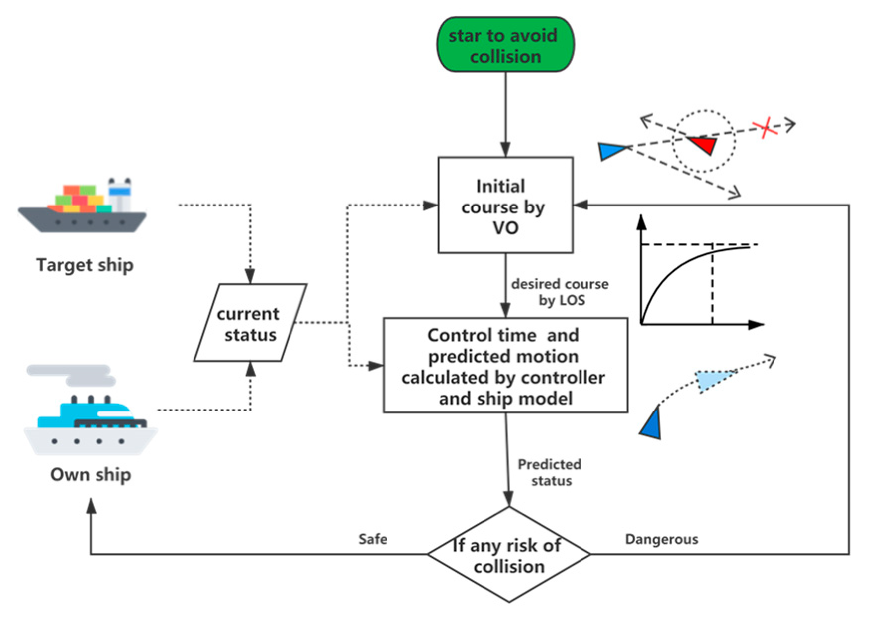
5.5. The Whole Framework of the System

This section describes the working orders of each modules of the whole system, as shown in the Figure 11, the whole system will start in a fixed interval, the own ship navigates in three shifts, avoiding collisions, keeping course and returning to route, the system will start in equal interval by checking the completion of the previous task by comparing the difference between the current heading and the desired. If the course is close to the desired within an allowable error, indicating the previous task is completed, collision detection starts. The collision avoidance module begins to work when there is any risk of collision, otherwise the returning module checks whether the situation is feasible to return to nest scheduled waypoint. The green colored collision avoidance sub-system is demonstrated in Figure 12, blue sub-system of returning is demonstrated in Figure 13.

The difference between the collision avoidance and returning module is that the returning module will make sure that own ship is not in a large crossing encounter, if own ship is close to parallel with the targeted ship, a large angle of desired course change will be set.

6. Experiment Results

6.1. Single Obstacles

Experiments are conducted by a single static obstacle and a single targeted ship to examine the effectiveness of the coordination between the decision and the controlling systems.

To clearly show that the comparative ship with traditional method enters the safety domain, the radius of all the safety domain is set as 0.5 nautical mile (926 m). For better illustration the unit are set as meter in this section.

The Figure 14 shows the results of avoiding single static obstacle, initial position of own ship is (0, 3000), the center location of the static obstacle is (2000, 3000), the unit is meter. The velocity of own ship is 15.5 kn, initial course 090. The gray area of polygon denotes an obstacle and the red circle is its safety domain. The black solid curve is the trajectory of own ship with coordination system while the dashed with normal method of VO algorithm.

The diagrams indicate that the ship with the proposed algorithm can avoid collision following more propriate course outside of the safety domain in contrast to the ship with simple VO algorithm. This is because the tradition method does not take the maneuverability into consideration. The desired course of proposed method is relatively larger (127.1° in contrast to 117.2°). The control angle is limited within $\pm 35°$, and does not step too quick.

The Figure 15 presents the results of collision avoidance by single targeted ship with the time point of 40 s, 295 s and 500 s. The initial position of own ship is (0, 3000), the targeted ship starts at (3800, 3000), the unit is meter, the velocity of own ship is 15.5 kn, and the targeted ship 10 kn, the initial course of own ship is 090, the course of the targeted ship is 270.

At the time point of 295 s in the Figure 15, the own ship with proposed algorithm passes the safety domain of the targeted ship without entering the domain, while the own ship with normal method intrudes the circle. As shown in the figure of course changing, the heading change by the proposed method is around 6° larger than that by simple VO.

As in Figure 16, the targeted ship is in a vertical crossing encounter situation with the own ship. The initial position of own ship is (0, 3000), the targeted ship starts at (2000, 3800), the unit is meter. The velocity of own ship is 15.5 kn, the targeted ship 6 kn. Initial course of own ship is 090, the targeted 180. At the time point of 260 s, the experiment shows the similar results to the previous test, the own ship takes a 8° larger heading change in contrast to the one with normal method, and this leads to intrusion of the safe domain.

6.2. Multiple Ships

In this section, a series of more complicated scenarios called “Imazu problem” are tested in larger ranges. Imazu problem [46] is a scenario set including tests from basic situations of two ships to complex 3–4 ships in encounter as shown in the following plot.

The starting location of own ship of all the 22 cases is set to the position of$\left(0,-6\right)$ the unity of which is nm (nautical mile), initial course 090, the velocities of all the ships are 11.7 kn with the exception in case 3, 7, 15, 20 and 22 where the overtaking situation happens, the targeted ship to be overtaken is set to navigate with the velocity of 7.8 kn. The goal waypoint for the own ship to return to is positioned at$\left(0,6\right)$ in each case. The targeted ships are in a distance of 6 nm to the center (0, 0) of the map but in different courses from 000 to 270, the simulation time is set to not more than 6000 s. Different form the former experiments, the unit of the distance is nm (nautical mile), each grid denotes 2 nm in the map. The safety domain radius is set to 0.5 nm much larger than that in former sections. The experiments are conducted in two groups, the group one is the comparative experiment with the proposed coordination system but without the large angle crossing problem correction, the COLREGS constraints are not applied either; In the group two, the collision avoidance is conducted with the proposed coordination system, the large crossing problem is solved and the COLREGS rule is also applied.

In the Figure 17, the experiment group one, some of the trajectories indicate that the own ship can avoid all the collisions in a generally reasonable manner. While in case 6, 10, 12, 13, 14 and 17 the own ship fails to return to the waypoint. This situation is caused by large angle crossing problem, the ship is out of collision danger, when it attempts to return, the collision detection function finds it not appropriate to change course, so the ship keeps its course all along the experiment. In case 6 and 10 the own ship is parallel to the targeted ship 1, in case 12, 13, 14 and 17 the ship is parallel to targeted ship 2; in case 9, 11, 18 and 20 the large angle crossing situation also happens, while the own ship is successful in returning to the waypoint because of the relative position change as the ships navigate, while the change is too slow in case 22 that the own ship takes long time to return.

In addition, there are left rudders in 10 cases (1, 4, 6, 9, 11, 12, 14, 16, 18 and 22) out of all the 22 scenarios, which does not match with navigation practices. This is usually caused by the targeted ships coming from the right side. Thus, the COLREGS are necessary to constrain the collision avoidance manners.

The Figure 18 shows the more mature maneuvering manners by the test trajectories. All the collisions are avoided by the own ship with successful returning to the waypoint. The large angle crossing situation problem is eliminated.

The rudder turning are improved according to the collision rule constrains, with only 5 cases (6, 12, 14, 18, 20) turning to left. Our analysis is that the targeted ship is on the right side and too close to the own ship (e.g., in case 6, 12, 14, the initial targeted ship is in less than 1 nm, in case 18 and 20 the nearest targeted ship is in less than 2 nm). The own ship is allowed to turn to left if the situation is in an urgent situation without violating the COLREGS.

To make comparison in more details, the comparisons between trajectories before modification by large cross situation and COLREGs constraints and the modified version of case 6 (Figure 19), case 4 (Figure 20) and case 22 (Figure 21) are illustrated.

Another two sets of experiments are conducted with more than 4 targeted ships, in Figure 22, we make up a scenario by cases of 2, 3, 4, 6 and 10. In Figure 23 we set a scenario with 7 targeted ships heading in various directions which is different from all the Imazu problems.

The Figure 23 show the most complicated encounter situations with more than 5 vessels encountering. with the simulation time point of 1700s, 3400s and 5100s. The own ship is in various encounter situations with the targeted ships. The own ship turns on starboard rudder. The good manners of autonomous collision avoidance indicate the effectiveness of the proposed approaches.

7. Discussions

The prediction accuracy is of great importance in the proposed coordination system, which needs the ship motion model and controller model to give the future status of own ship, thus the two models will always involve in the whole system. The prediction error will always exist and contributes to the problem of predictions. To be close to the reality, we imposed a simple error of 10% on the autopilot so that the ship heading will never be exactly controlled to the ordered course, although the outcomes of the experiment is satisfied, we infer that this is because the disturbance is not large enough. There is not any model that could predict the ship maneuverability with little error, However, the advantage of using models is that instead of searching an optimum in a random space, it could give initial information as references for initial decision making and describe the maneuverability of ships to some extent.

The validation of collision avoidance algorithm will always need reasonable testing scenarios. The Imazu [46] problems offer a bunch of situations. The withdraw is that all the targeted ships will pass through the center of the map, resulting them actually colliding at the center, which will never happen in reality. The initial layout of the targeted ships in case 6, 12, 13, etc. are too close even less than 1 nm to the own ship, leading the experiment starting in an urgent situation. Even though Imazu problem has scenarios as many as 22 cases, much more testing sets are needed to check the effectiveness of the proposed algorithm. All the targeted ships are set on fixed velocity and heading, which is not the situations at sea.

For the collision avoiding manners abiding COLREGs, the own ships in 5 out of the 22 cases turn to left rudder because of the coming targeted ships form the right side with the distance less than 2 nm, this is reasonable in navigation practice. In some cases (e.g., 8, 10, 11, 16) the own ship avoids collision by passing the bow of targeted ship. This implies that crossing the bow will also be carried out if the circumstance is safe enough.

The cycle interval of the system is undetermined in the work, we set that the system will start to function after every 20 s. If the time is too short, the ship will continuously get orders from the decision-making with the previous tasks uncompleted, the ship will not respond immediately because it cannot change status substantially in a very short time and the computation requirement is relatively heavy. On the contrary, if the time is too long, obviously the own ship may neglect potential risk or timing for returning.

8. Conclusions

Ships may deviate from its expected trajectory when avoiding collisions by changing its heading. If they are in large size with high inertia, there is an obvious lag between the controlling and the decision system. Aimed at the problem, a coordination system is designed to cover the gap and help for effective collision avoidance and returning to the waypoints in various encounter scenarios.

The controller is designed to work in a more practical manner. DCPA and the distance between other ships are involved to detect risk of collision for the timing of decision making; the situation dividing according to COLREGS are simplified to restrict the course changing direction; based on VO and LOS method, the collision avoidance and returning to the scheduled waypoint are accomplished, the VO method is modified by a recursive prediction algorithm while the LOS guidance is improved by large angle crossing function, All the parts above form a coordination system for autonomous collision avoidance system. The series of experiments including Imazu problem are conducted to test the effectiveness of the proposed algorithm.

The future research should be focused on the testing and validating of an autonomous ship, autonomous ship techniques have been developing rapidly, the demand is increasing to check if these algorithms have an extensive coverage of various conditions, this would be related to many other aspects, such as modelling and simulation, software test, performance evaluation, etc.

References

1. Huang, Y.; van Gelder, P.H.A.J.M. Time-Varying Risk Measurement for Ship Collision Prevention. Risk Anal. 2020, 40, 24–42. [Google Scholar] [CrossRef] [PubMed]
2. Gao, Z.J.; Zhang, Y.J.; Sun, P.T.; Li, W.H. Research Summary of Unmanned Ship. Dalian Haishi Daxue Xuebao J. Dalian Marit. Univ. 2017, 43, 1–7. [Google Scholar]
3. Yan, X.; Wang, S.; Ma, F.; Yan, X.; Wang, S.; Ma, F. Review and Prospect for Intelligent Cargo Ships. Chin. J. Ship Res. 2021, 16, 1–6. [Google Scholar] [CrossRef]
4. Lyu, H.; Yin, Y. COLREGS-Constrained Real-Time Path Planning for Autonomous Ships Using Modified Artificial Potential Fields. J. Navig. 2019, 72, 588–608. [Google Scholar] [CrossRef]
5. Wang, C.; Zhang, X.; Cong, L.; Li, J.; Zhang, J. Research on Intelligent Collision Avoidance Decision-Making of Unmanned Ship in Unknown Environments. Evol. Syst. 2019, 10, 649–658. [Google Scholar] [CrossRef]
6. Hu, Y.; Meng, X.; Zhang, Q.; Park, G.K. A Real-Time Collision Avoidance System for Autonomous Surface Vessel Using Fuzzy Logic. IEEE Access 2020, 8, 108835–108846. [Google Scholar] [CrossRef]
7. Su, C.M.; Chang, K.Y.; Cheng, C.Y. Fuzzy Decision on Optimal Collision Avoidance Measures for Ships in Vessel Traffic Service. J. Mar. Sci. Technol. 2012, 20, 5. [Google Scholar] [CrossRef]
8. Nomoto, K.; Taguchi, K.; Honda, K.; Hirano, S. On the Steering Qualities of Ships. J. Zosen Kiokai 1956, 1956, 75–82. [Google Scholar] [CrossRef]
9. Zhang, J.; Yan, X.; Chen, X.; Sang, L.; Zhang, D. A Novel Approach for Assistance with Anti-Collision Decision Making Based on the International Regulations for Preventing Collisions at Sea. Proc. Inst. Mech. Eng. Part M J. Eng. Marit. Environ. 2012, 226, 250–259. [Google Scholar] [CrossRef]
10. Wang, B.; He, Y.; Hu, W.; Mou, J.; Li, L.; Zhang, K.; Huang, L. A Decision-Making Method for Autonomous Collision Avoidance for the Stand-on Vessel Based on Motion Process and Colregs. J. Mar. Sci. Eng. 2021, 9, 584. [Google Scholar] [CrossRef]
11. Kadir, R.E.A.; Sahal, M.; Gamayanti, N.; Pratama, F.I. Dynamic Path Planning of Unmanned Surface Vehicle Based On Genetic Algorithm With Sliding Curve Guidance System. JAREE J. Adv. Res. Electr. Eng. 2021, 5, 47–56. [Google Scholar] [CrossRef]
12. Guo, X.; Ji, M.; Zhao, Z.; Wen, D.; Zhang, W. Global Path Planning and Multi-Objective Path Control for Unmanned Surface Vehicle Based on Modified Particle Swarm Optimization (PSO) Algorithm. Ocean Eng. 2020, 216, 107693. [Google Scholar] [CrossRef]
13. Wang, H.; Guo, F.; Yao, H.; He, S.; Xu, X. Collision Avoidance Planning Method of USV Based on Improved Ant Colony Optimization Algorithm. IEEE Access 2019, 7, 52964–52975. [Google Scholar] [CrossRef]
14. Shen, H.; Hashimoto, H.; Matsuda, A.; Taniguchi, Y.; Terada, D.; Guo, C. Automatic Collision Avoidance of Multiple Ships Based on Deep Q-Learning. Appl. Ocean Res. 2019, 86, 268–288. [Google Scholar] [CrossRef]
15. Johansen, T.A.; Perez, T.; Cristofaro, A. Ship Collision Avoidance and COLREGS Compliance Using Simulation-Based Control Behavior Selection with Predictive Hazard Assessment. IEEE Trans. Intell. Transp. Syst. 2016, 17, 3407–3422. [Google Scholar] [CrossRef] [Green Version]
16. Borkowski, P.; Zwierzewicz, Z. Ship Course-Keeping Algorithm Based on Knowledge Base. Intell. Autom. Soft Comput. 2013, 17, 149–163. [Google Scholar] [CrossRef]
17. Sun, X.; Wang, G.; Fan, Y.; Mu, D.; Qiu, B. Collision Avoidance Using Finite Control Set Model Predictive Control for Unmanned Surface Vehicle. Appl. Sci. 2018, 8, 926. [Google Scholar] [CrossRef] [Green Version]
18. Kozynchenko, A.I.; Kozynchenko, S.A. Applying the Dynamic Predictive Guidance to Ship Collision Avoidance: Crossing Case Study Simulation. Ocean Eng. 2018, 164, 640–649. [Google Scholar] [CrossRef]
19. Borkowski, P.; Pietrzykowski, Z.; Magaj, J. The Algorithm of Determining an Anti-Collision Manoeuvre Trajectory Based on the Interpolation of Ship’s State Vector. Sensors 2021, 21, 5332. [Google Scholar] [CrossRef]
20. Fossen, T.I. Handbook of Marine Craft Hydrodynamics and Motion Control; John Wiley & Sons: Hobeken, NJ, USA, 2011. [Google Scholar]
21. Tsourdos, A.; White, B.; Shanmugavel, M. Cooperative Path Planning of Unmanned Aerial Vehicles; John Wiley & Sons: Hobeken, NJ, USA, 2010. [Google Scholar]
22. Lisowski, J. Synthesis of a Path-Planning Algorithm for Autonomous Robots Moving in a Game Environment during Collision Avoidance. Electronics 2021, 10, 675. [Google Scholar] [CrossRef]
23. Zhao, L.; Roh, M.-I.; Lee, S.-J. Control method for path following and collision avoidance of autonomous ship based on deep reinforcement learning. J. Mar. Sci. Technol. 2019, 27, 1. [Google Scholar] [CrossRef]
24. Liu, Y.; Bu, R.; Gao, X. Ship Trajectory Tracking Control System Design Based on Sliding Mode Control Algorithm. Pol. Marit. Res. 2018, 3, 26–34. [Google Scholar] [CrossRef] [Green Version]
25. Abdelaal, M.; Fränzle, M.; Hahn, A. Nonlinear Model Predictive Control for Trajectory Tracking and Collision Avoidance of Underactuated Vessels with Disturbances. Ocean Eng. 2018, 160, 168–180. [Google Scholar] [CrossRef]
26. Feng, Y.-X.; Zhang, X.-K. An Improved Control Algorithm for Ship Course Keeping Based on Nonlinear Feedback and Decoration. In Proceedings of the 37th Chinese Control Conference (CCC), Wuhan, China, 25–27 July 2018; pp. 297–303. [Google Scholar] [CrossRef]
27. Zhang, Q.; Zhang, X.-K.; Im, N.-K. Ship Nonlinear-Feedback Course Keeping Algorithm Based on MMG Model Driven by Bipolar Sigmoid Function for Berthing. Int. J. Nav. Archit. Ocean Eng. 2017, 9, 525–536. [Google Scholar] [CrossRef]
28. Källström, C.; Åström, K.J.; Byström, L.; Norrbin, N.H. Further Studies of Parameter Identification of Linear and Nonlinear Ship Steering Dynamics; The Swedish State Shipbuilding Experimental Tank: Report 1920-6; Statens Skeppsprovningsanstalt: Gothenburg, Sweden, 1977. [Google Scholar]
29. Witkowska, A.; Tomera, M.; Śmierzchalski, R. A Backstepping Approach to Ship Course Control. Int. J. Appl. Math. Comput. Sci. 2007, 17, 73–85. [Google Scholar] [CrossRef] [Green Version]
30. Zhang, X.K.; Zhang, Q.; Ren, H.X.; Yang, G.P. Linear Reduction of Backstepping Algorithm Based on Nonlinear Decoration for Ship Course-Keeping Control System. Ocean Eng. 2018, 147, 1–8. [Google Scholar] [CrossRef]
31. Pierson, W.J.; Moskowitz, L. A Proposed Spectral Form for Fully Developed Wind Seas Based on the Similarity Theory of S. A. Kitaigorodskii. J. Geophys. Res. 1964, 69, 5181–5190. [Google Scholar] [CrossRef]
32. Min, B.; Zhang, X.; Wang, Q. Energy Saving of Course Keeping for Ships Using CGSA and Nonlinear Decoration. IEEE Access 2020, 8, 141622–141631. [Google Scholar] [CrossRef]
33. Baran, A.; Fiskin, R.; Kiźi, H. A Research on Concept of Ship Safety Domain. TransNav Int. J. Mar. Navig. Saf. Sea Transp. 2018, 12, 43–47. [Google Scholar] [CrossRef]
34. Fujii, Y.; Tanaka, K. Traffic Capacity. J. Navig. 1971, 24, 543–552. [Google Scholar] [CrossRef]
35. Xu, Q.; Wang, N. A Survey on Ship Collision Risk Evaluation. Promet—Traffic Transp. 2014, 26, 475–486. [Google Scholar] [CrossRef]
36. Park, J.; Jeong, J.-S. An Estimation of Ship Collision Risk Based on Relevance Vector Machine. J. Mar. Sci. Eng. 2021, 9, 538. [Google Scholar] [CrossRef]
37. Shaobo, W.; Yingjun, Z.; Lianbo, L. A Collision Avoidance Decision-Making System for Autonomous Ship Based on Modified Velocity Obstacle Method. Ocean Eng. 2020, 215, 107910. [Google Scholar] [CrossRef]
38. Lyu, H.; Yin, Y. Ship’s Trajectory Planning for Collision Avoidance at Sea Based on Modified Artificial Potential Field. In Proceedings of the 2017 2nd International Conference on Robotics and Automation Engineering (ICRAE 2017), Shanghai, China, 29–31 December 2018; Volume 2017. [Google Scholar]
39. Sawada, R.; Sato, K.; Majima, T. Automatic Ship Collision Avoidance Using Deep Reinforcement Learning with LSTM in Continuous Action Spaces. J. Mar. Sci. Technol. 2021, 26, 509–524. [Google Scholar] [CrossRef]
40. Zaccone, R. COLREG-Compliant Optimal Path Planning for Real-Time Guidance and Control of Autonomous Ships. J. Mar. Sci. Eng. 2021, 9, 405. [Google Scholar] [CrossRef]
41. Tam, C.; Bucknall, R. Collision Risk Assessment for Ships. J. Mar. Sci. Technol. 2010, 15, 257–270. [Google Scholar] [CrossRef]
42. Ding, Z.; Zhang, X.; Wang, C.; Li, Q.; An, L.; Ding, Z.; Zhang, X.; Wang, C.; Li, Q.; An, L. Intelligent Collision Avoidance Decision-Making Method for Unmanned Ships Based on Driving Practice. Chin. J. Ship Res. 2021, 16, 96–104; 113. [Google Scholar] [CrossRef]
43. Huang, Y.; Chen, L.; van Gelder, P.H.A.J.M. Generalized Velocity Obstacle Algorithm for Preventing Ship Collisions at Sea. Ocean Eng. 2019, 173, 142–156. [Google Scholar] [CrossRef]
44. Chen, P.; Huang, Y.; Mou, J.; van Gelder, P.H.A.J.M. Ship Collision Candidate Detection Method: A Velocity Obstacle Approach. Ocean Eng. 2018, 170, 186–198. [Google Scholar] [CrossRef]
45. Cho, Y.; Han, J.; Kim, J. Efficient COLREG-Compliant Collision Avoidance in Multi-Ship Encounter Situations. IEEE Trans. Intell. Transp. Syst. 2020, 2020, 1–13. [Google Scholar] [CrossRef]
46. Imazu, H. Research on Collision Avoidance Manoeuvre; Tokyo University of Marine Science and Technology: Tokyo, Japan, 1987. [Google Scholar]
Figure 1. Comparison among ship headings controlled by Backstepping (a), CGSA (b) and pure PID (c).
Jmse 09 01202 g001
Figure 2. Comparison among ship controller outputs (rudders) by Backstepping (a), CGSA (b) and pure PID (c).
Jmse 09 01202 g002
Figure 3. Detection range.
Jmse 09 01202 g003
Figure 4. Encounter situation division.
Jmse 09 01202 g004
Figure 5. VO algorithm principles; (a) Basic VO algorithm; (b) VO algorithm for multiple targeted ships.
Jmse 09 01202 g005
Figure 6. Procedures of collision avoiding algorithm; (a) Sketchmap of collision avoidance algorithm; (b) Flowchart of collision avoidance algorithm.
Jmse 09 01202 g006
Figure 7. Procedures of returning to waypoint algorithm. Initial tries to return to the waypoint by LOS in (a) and (b) are failed due to time delay by large inertia. By applying the proposed returning algorithm, the ship in (c) keeps its course and then predicted the ship status in (d) and finally returns to the way point properly.
Jmse 09 01202 g007
Figure 8. Flowchart of returning to waypoint algorithm.
Jmse 09 01202 g008
Figure 9. Large crossing problem and practices in navigation to solve the problem.
Jmse 09 01202 g009
Figure 10. Diagram of proposed method identifying the large crossing situation.
Jmse 09 01202 g010
Figure 11. Framework of the whole system.
Jmse 09 01202 g011
Figure 12. Framework of the collision avoidance module.
Jmse 09 01202 g012
Figure 13. Framework of the returning to waypoint module.
Jmse 09 01202 g013
Figure 14. Experiment on single static obstacle. Ship trajectory by time of 70 s (a) and 340 s (b). The rudder angle (c) and the heading angle are shown in diagram (c,d).
Jmse 09 01202 g014
Figure 15. Experiment on single targeted ship with head on encounter. Ship trajectory by time of 40 s (a), 295 s (b) and 500 (c), the heading angle is shown in (d).
Jmse 09 01202 g015
Figure 16. Experiment on single targeted ship with crossing encounter. Ship trajectory by time of 200 s (a), 260 s (b) and 400 s (c). The heading angle is shown in (d).
Jmse 09 01202 g016
Figure 17. Experiment on Imazu scenarios (group 1).
Jmse 09 01202 g017
Figure 18. Experiment on Imazu scenarios (group 2).
Jmse 09 01202 g018
Figure 19. Comparison of case 6 for eliminating the large angle crossing problem. in the subfigure (a), heading of the own ship keeps its course close to the blue trajectory of the targeted ship and fails to return to the waypoint, the problem is solved in subfigure (b), the ship keeps its course firstly and then identify the large crossing situation, with its heading changes to the other side in a large angle, finally return to the way point successfully. The heading angles of subfigure (a,b) are shown in (c,d).
Jmse 09 01202 g019
Figure 20. Comparison of case 4 for constraining the course change by COLREGS, the course is in a left rudder in subfigure (a), in subfigure (b), it can be found that the own ship takes longer time to return to the waypoint, this is because the initial heading is close to the targeted ship, the large angle crossing situation forms, the ship steers in a large turn on the right side and then finds its way back to the waypoint. The heading angles of (a,b) are shown in (c,d).
Jmse 09 01202 g020
Figure 21. Comparison of case 22 for constraining the course changing by COLREGS. the course is in a left rudder in subfigure (a), in subfigure (b) the starboard rudder is applied, which abides the rule in practice. The heading angles of (a,b) are shown in (c,d).
Jmse 09 01202 g021
Figure 22. A scenario that combines the case 2, 3, 4, 6 and 10, the own ship navigates to starboard side with a minor vibration of is heading initially and then return to the waypoint. Ship trajectory is shown by time of 1400 s (a), 2800 s (b) and 4200 s (c), the heading angle is shown in subfigure (d).
Jmse 09 01202 g022aJmse 09 01202 g022b
Figure 23. Experiment on 7 targeted ships. Ship trajectory is shown by time of 1700 s (a), 3400 s (b) and 5100 s (c), the heading angle is shown in subfigure (d).
Jmse 09 01202 g023