Pipeline Pressure Loss in Deep-Sea Hydraulic Systems Considering Pressure-Dependent Viscosity Change of Hydraulic Oil

Abstract

The high ambient pressure in deep-sea conditions greatly increases the viscosity of hydraulic oil and then the pipeline pressure loss in deep-sea hydraulic systems. Large pipeline pressure loss can lead to a further change of viscosity on the basis of the viscosity increase caused by the ambient pressure when the hydraulic oil flows through the pipeline. Therefore, the classic Poiseuille’s law can no longer accurately calculate the pipeline pressure loss in deep-sea conditions since it treats the viscosity as a constant. In this paper, based on laminar flow theory and the viscosity-pressure characteristics of hydraulic oil, a novel equation for pipeline pressure loss is proposed, in which the viscosity change when flowing through the pipeline is taken into account. A CFD (Computational Fluid Dynamics) model of a pipeline in the deep-sea hydraulic system has been established, and CFD simulations have been conducted to verify the correctness of the proposed equation for pipeline pressure loss. Theoretical analysis shows that the proposed novel equation for pipeline pressure loss is equivalent to the classic Poiseuille’s law when the pipeline pressure loss or the viscosity change is low. The research results in this paper can provide theoretical support for work efficiency optimization, load capacity improvement, and precise control of deep-sea operation equipment or deep-sea hydraulic systems.

1. Introduction

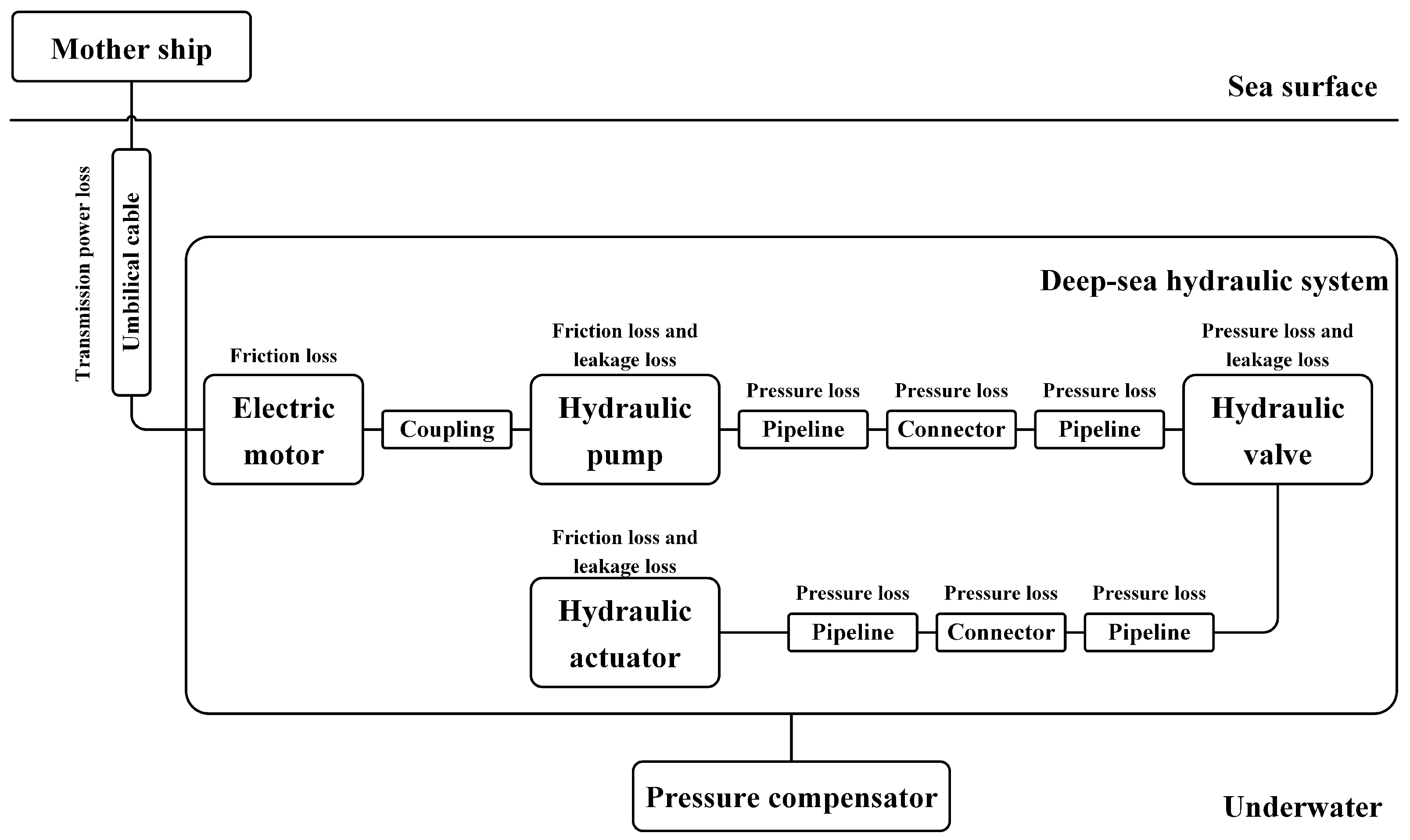
Various deep-sea operation equipment, such as human occupied vehicles (HOVs) [1], remotely operated vehicles (ROVs) [2], submarine mining vehicles [3,4], autonomous underwater vehicles (AUVs) [5], and submarine cable trenchers [6], have been successfully designed and developed. In addition, with them, humans have carried out much scientific exploration and resource development in the deep-sea environment. These high-power deep-sea operation equipment are usually powered by a motor-driven hydraulic system [7,8], and the power is provided by the mother ship on the sea surface through an umbilical cable, as shown in Figure 1. The loss in each power transmission link is also indicated in Figure 1.

The deep-sea hydraulic system is equipped with a pressure compensator [9,10,11], which introduces the seawater ambient pressure that increases with depth into the hydraulic system. Then, the internal and external pressures of the hydraulic system tend to be balanced. Therefore, the components in the deep-sea hydraulic system do not need to be designed with a special pressure-resistant structure, and the mature technology in the land hydraulic system can be transplanted and applied. As a result, the development and design costs of the deep-sea hydraulic system can be greatly reduced.

However, the viscosity of hydraulic oil increases exponentially with pressure. Hydraulic oil is the energy transfer medium of the hydraulic system. Therefore, the increase in its viscosity would cause the loss of each transmission link in the deep-sea hydraulic system to increase significantly compared with those in land conditions. Furthermore, the working efficiency, load driving capability, and precise control of deep-sea operation equipment are seriously affected. Some scholars have researched the influence on deep-sea hydraulic systems caused by the viscosity increase of hydraulic oil.

Cao et al. [12] established a deep-sea hydraulic power unit model based on the linear varying parameters modeling method, which considered the compressibility and viscosity of hydraulic oil affected by ambient pressure in the deep-sea environment. Based on the established model, simulation analysis was carried out to predict the dynamic performance of the hydraulic power unit, which was verified by experimental tests. Tian et al. [13] developed a mathematical model of the pressure control variable displacement pump, which is the power source of the deep-sea hydraulic manipulator. In the model, the increased viscosity of the hydraulic oil caused by the ambient pressure of the seawater was considered. The influence of the viscosity on the dynamic characteristics and performance of the pump was simulated and corresponding experiments were conducted. Tian et al. [14] tested the change in hydraulic oil viscosity with pressure and established a nonlinear model of an underwater manipulator that took into account the increase in hydraulic oil viscosity caused by ambient pressure. Then, the influence of ambient pressure on the dynamic performance of the manipulator was studied, and the online test under the ambient pressure of 115 MPa was carried out.

In the performance analysis of the land hydraulic system, the dynamic process and pressure loss of the connecting pipeline are ignored to simplify the model [15,16]. Under the effect of the high ambient pressure in the deep sea, the viscosity of hydraulic oil increases significantly, and then the pipeline pressure loss cannot be ignored directly. Deep-sea operation equipment usually has multiple actuators in concert, and many actuators are distributed far away from the hydraulic pump. As a result, there are numerous long-distance pipelines in the deep-sea hydraulic system. Therefore, the pipeline pressure loss has a significant impact on the operation of deep-sea operation equipment. The flow in the pipeline is generally a typical Poiseuille flow, and many scholars have carried out related studies on the Poiseuille flow or pipeline pressure loss.

Savić et al. [17] developed a numerical model for determining the pressure losses within flat pipelines. In this numerical model, the influence of pressure and temperature on the density and viscosity of the oil was taken into account. Ganji et al. [18] utilized the Arrhenius model to describe the temperature-viscosity characteristics of the fluid and researched the steady-state Hagen-Poiseuille flow in a circular pipe. Housiadas and Georgiou [19] assumed that density and the viscosity of the fluid have a linear relationship with pressure, and then proposed a novel solution for Poiseuille flows. Based on a Runge–Kutta–Fehlberg integration scheme with shooting technique, Makinde et al. [20] investigated a magnetohydrodynamic Couette-Poiseuille flow between two parallel plates in a rotating permeable channel, in which the temperature-viscosity characteristics of the fluids was taken into account. Lee et al. [21] studied how surface roughness affects the flow characteristics, and the result showed that the roll mode for the Couette-Poiseuille flow over a rough wall can be inhibited by the surface roughness. Hong-Xiang [22] calculated the pipeline pressure loss in the deep-sea hydraulic system, taking into account the increase in viscosity caused by high pressure and low temperature in deep-sea conditions. Then, a variable gain control algorithm of the underwater manipulator based on the pressure loss was developed, which was verified through simulation and experimental testing. With numerical methods, Luo et al. [23] studied the propagation of Taylor vortices in Taylor-Couette-Poiseuille flow considering the effects of an abruptly contracting and expanding annular gap. Li and Wu [24] researched the deformation and leakage mechanisms at hydraulic clearance fit in the deep-sea extreme environment, in which the viscosity-pressure characteristics of hydraulic oil was considered. With the Chebyshev collocation and the Galerkin methods, B.M. and Shivakumara [25] researched how the uniform vertical throughflow affects the stability of Poiseuille flow in a Newtonian fluid-saturated Brinkman porous medium.

Generally, the pressure loss in the pipeline can be determined by Poiseuille’s law.

$$\Delta p=\frac{128\eta LQ}{\pi D^4},$$

(1)

where $\Delta p$ is the pressure loss, $\eta$ is the viscosity, L and D are the length and the inner diameter of the pipeline, respectively, and Q is the flow rate.

The viscosity-pressure characteristics of hydraulic oil can be fitted by the Barus formula [26], which is expressed as Equation (2).

$$\eta ={\eta }_0{e}^{\alpha p_o},$$

(2)

where ${\eta }_0$ is the initial viscosity of the oil at standard atmospheric pressure, $\alpha$ is the viscosity-pressure index, and $p_o$ is the outlet pressure of the pipeline. Due to the function of the pressure compensator, for an inflow pipeline that connects the hydraulic pump and the hydraulic actuator, $p_o$ is the sum of the ambient pressure and the load pressure. As for the return pipeline that connects the hydraulic actuator and the oil tank, $p_o$ equals ambient pressure.

With Equations (1) and (2), the pressure loss considering the viscosity increase caused by the extremely high ambient pressure in the deep sea is obtained as follows.

$$\Delta p=\frac{128{\eta }_{0}LQ{e}^{\alpha p_o}}{\pi D^4}.$$

(3)

The fluid viscosity in Equation (1) is a constant value. In Equation (3), the viscosity takes into account the change caused by ambient pressure, but it is still a constant value when the hydraulic oil flows through the pipeline. When in land conditions or shallow sea conditions, the ambient pressure is tiny, and so are the outlet pressure of the pipeline $p_o$ and the pressure loss calculated by Equation (3). Therefore, the viscosity of the hydraulic oil changes minimally, and the calculation using Equation (3) is still reasonable.

However, when working in deep-sea conditions, the viscosity of hydraulic oil is greatly increased compared with land working conditions, so the pipeline pressure loss also increases significantly, which can exceed 10 MPa. Such a huge internal loss in the system seriously reduces the working efficiency of deep-sea operation equipment or deep-sea hydraulic systems. Generally, the maximum output pressure of the hydraulic pump usually does not exceed 30 MPa. Therefore, the pipeline pressure loss of up to 10 MPa reduces the load capacity of the deep-sea hydraulic system by an incredible 33%. In addition, proportional valves or servo valves are usually used in hydraulic systems to achieve high-precision control. For a proportional valve or servo valve with a given control signal, the flow rate that flows through it to the hydraulic actuator is related to the pressure difference between the inlet and outlet of the valve [14,16]. When the deep-sea hydraulic system works at different depths, the viscosity of the hydraulic oil changes and so does the pipeline pressure loss, which results in the variations of the pressure difference between the inlet and outlet of the valve and, furthermore, the flow rate to the hydraulic actuator. As a consequence of this series of changes, the hydraulic actuators have different output responses at different underwater depths, even with the same control signal, which is very unfavorable for the precise control. The above analysis shows that pipeline pressure loss has a significant influence on the work efficiency, load capacity, and precise control of deep-sea operation equipment or deep-sea hydraulic systems.

Besides, a pressure loss of 10 MPa can cause a significant change in the viscosity of the hydraulic oil when flowing through the pipeline. Taking $\alpha$ as $2.2\times {10}^{-8}$ Pa${}^{-1}$, the change percentage in hydraulic oil viscosity caused by a pressure loss of 10 MPa can be calculated using Equation (2), which is

$$\frac{{\eta }_0{e}^{\alpha (p_o+\Delta p)}-{\eta }_0{e}^{\alpha p_o}}{{\eta }_0{e}^{\alpha p_o}}\times 100\%=\left(e^{\alpha \Delta p}-1\right)\times 100\%=\left(e^{2.2\times {10}^{-8}\mathrm{P}{\mathrm{a}}^{-1}\times 10\mathrm{MPa}}-1\right)\times 100\%=24.61\%.$$

(4)

Equation (4) indicates that the viscosity of the hydraulic oil flowing through the pipeline changes by as much as 24.61%, which means that the classical Poiseuille’s law, in which the viscosity is treated as a constant value, can no longer accurately calculate the pipeline pressure loss in the deep-sea hydraulic system.

However, few studies involved pipeline pressure loss in deep-sea hydraulic systems. In addition, the corresponding research only considered the increase in viscosity caused by the ambient pressure of the deep-sea environment, instead of the viscosity change during the flowing process, as in the research of Tian et al. [14] and Hong-Xiang [22]. Therefore, it is necessary to conduct an in-depth study on the pipeline pressure loss in the deep-sea hydraulic system, in which the viscosity change of the hydraulic oil during the flowing process in the pipeline should be taken into account.

In this paper, based on laminar flow theory and the viscosity-pressure characteristics of hydraulic oil, a novel equation for pipeline pressure loss is derived, in which fluid viscosity is variable. Then, a CFD model of a pipeline in the deep-sea hydraulic system is established, and simulations are carried out to verify the correctness of the proposed novel equation for pipeline pressure loss. Finally, the proposed novel equation for pipeline pressure loss is analyzed and discussed, and it is also compared with the classic Poiseuille’s law. The research results in this paper can provide theoretical support for work efficiency optimization, load capacity improvement, and precise control of deep-sea operation equipment or deep-sea hydraulic systems.

2. Theory Analysis

Laminar flow has less energy loss than turbulent flow. Therefore, in the design of the hydraulic system, according to the volume flow rate and the set maximum average flow velocity, the pipe diameter can then be determined so that the hydraulic oil flows in a laminar flow state in the pipeline [27]. Therefore, in this paper, the laminar fluid domain in the circular pipeline is used for analysis, and the analysis model is shown as Figure 2. A micro-cylinder with a length of $dl$ and a radius of r located on the axis of the pipeline is selected as the research object. The outlet pressure of the micro-cylinder is p, the pressure loss when flowing through the micro-cylinder is $dp$, and the flow velocity on the surface of the micro-cylinder is v.

The pipeline model in Figure 2 is placed horizontally. The diameter of the pipeline usually does not exceed 100 mm. Based on the hydraulic oil density of 850 $\mathrm{kg}/{\mathrm{m}}^3$, the pressure difference between the upper and lower hydraulic oil in the pipeline due to gravity is

$$850\mathrm{kg}/{\mathrm{m}}^3\times 9.8\mathrm{N}/\mathrm{kg}\times 100\mathrm{mm}=8.33\times 10^{-4}\mathrm{MPa},$$

which is very low. Therefore, for the horizontal model shown in Figure 2, gravity can be ignored.

When the pipeline is placed vertically, the pressure difference due to gravity in a pipeline with a length of 5 m is

$$850\mathrm{kg}/{\mathrm{m}}^3\times 9.8\mathrm{N}/\mathrm{kg}\times 5\mathrm{m}=4.165\times 10^{-2}\mathrm{MPa},$$

which is far less than the pressure loss due to the viscosity of the hydraulic oil. Therefore, the results derived from the horizontal pipeline model in this paper are also applicable to vertical pipelines. Furthermore, it is obviously applicable to inclined pipes, as well.

The influence of temperature on viscosity is not considered in this analysis, and it is assumed that the hydraulic system is operating at a design condition of 40 °C.

When in the state of laminar flow, the fluids flow in the axial direction without interfering with each other. Therefore, in the radial direction, the forces of the micro-cylinder are balanced. In the axial direction, the micro-cylinder is subjected to the forces caused by pressure at both ends and the viscous friction force caused by the rest of the fluid on its surface, which are expressed as follows.

$$\left\{\begin{array}{c}{F}_i=\pi r^2(p+dp),\hfill \\ F_o=\pi r^{2}p,\hfill \\ F_f=A·\left(\eta \frac{dv}{dr}\right)=2\pi r\eta ·dl·\frac{dv}{dr}.\hfill \end{array}\right.$$

(5)

where $F_i$ and $F_o$ are the forces caused by pressure at the inlet and outlet, respectively, $F_f$ is the viscous friction force, and A is the side area of the micro-cylinder.

When the hydraulic oil in the pipeline is in the state of laminar flow, the axial forces of the micro-cylinder are also balanced. Then,

$$F_i=F_o+F_f,$$

(6)

or

$$\pi r^2(p+dp)=\pi r^{2}p+2\pi r\eta ·dl·\frac{dv}{dr},$$

(7)

or

$$dv=\frac{1}{2\eta }\frac{dp}{dl}rdr.$$

(8)

Substituting the viscosity-pressure characteristics expressed by Equation (2) into Equation (8) and replacing $p_o$ with p, we have

$$dv=\frac{1}{2{\eta }_0{e}^{\alpha p}}\frac{dp}{dl}rdr.$$

(9)

The inner radius of the pipeline is R, and the flow velocity here is 0. With these boundary conditions, we integrate and process Equation (9) as follows.

$${\int }_0^{v}dv={\int }_R^r\frac{1}{2{\eta }_0{e}^{\alpha p}}\frac{dp}{dl}rdr=\frac{1}{2{\eta }_0{e}^{\alpha p}}\frac{dp}{dl}{\int }_R^{r}rdr,$$

(10)

or

$$v=-\frac{R^2-r^2}{4{\eta }_0{e}^{\alpha p}}\frac{dp}{dl},$$

(11)

or

$$\frac{4v{\eta }_0}{R^2-r^2}dl=-e^{-\alpha p}dp.$$

(12)

The pipeline length is L and the outlet pressure of the pipeline is $p_o$. The inlet pressure is the sum of the outlet pressure $p_o$ and the pressure loss $\Delta p$. With these boundary conditions, we integrate and process Equation (12) as follows.

$${\int }_{-L}^0\frac{4v{\eta }_0}{R^2-r^2}dl=\frac{4v{\eta }_0}{R^2-r^2}{\int }_{-L}^{0}dl={\int }_{p_o+\Delta p}^{p_o}-e^{-\alpha p}dp,$$

(13)

or

$$\frac{4v{\eta }_{0}L}{R^2-r^2}=\frac{1}{\alpha }\left[e^{-\alpha p_o}-e^{-\alpha \left(p_o+\Delta p\right)}\right].$$

(14)

The flow velocity v can be obtained as follows by transforming Equation (14).

$$v=\frac{R^2-r^2}{4\alpha {\eta }_{0}L}\left[e^{-\alpha p_o}-e^{-\alpha \left(p_o+\Delta p\right)}\right].$$

(15)

According to Equation (15), the flow velocity v in the pipeline shows a quadratic parabolic distribution with the radius r, and the maximum flow velocity $v_{max}$, which is expressed as follows, occurs when r is 0, or on the axis.

$$v_{max}=\frac{R^2}{4\alpha {\eta }_{0}L}\left[e^{-\alpha p_o}-e^{-\alpha \left(p_o+\Delta p\right)}\right].$$

(16)

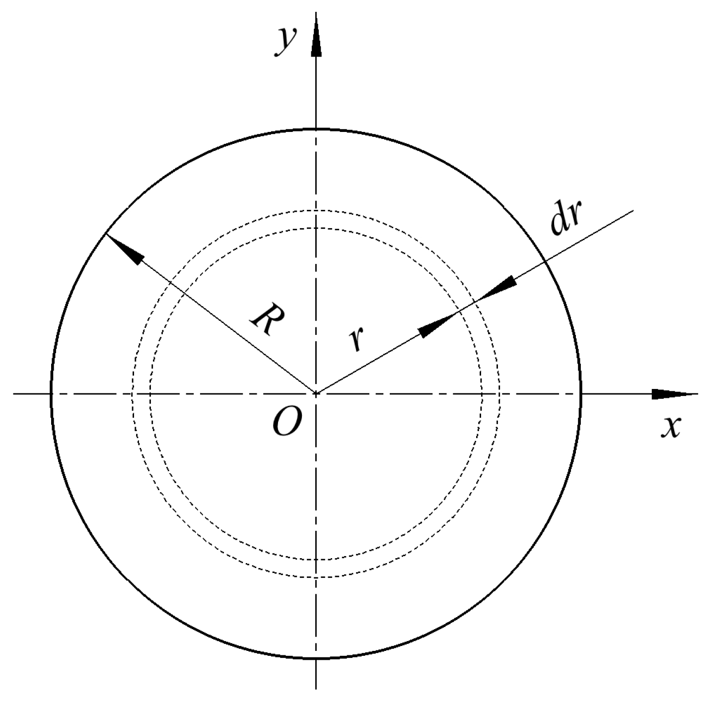
Based on Equation (15), the total flow rate of hydraulic oil in the pipeline can be derived. Figure 3 shows the pipeline cross-section. A micro-ring with radius r and width $dr$ in the cross-section is taken as the research object.

The flow rate through this micro-ring is

$$dQ=vdA=2\pi vrdr,$$

(17)

where $dA$ is the area of the micro-ring.

Substituting Equation (15) into Equation (17), we have

$$dQ=\frac{\pi }{2\alpha {\eta }_{0}L}\left[e^{-\alpha p_o}-e^{-\alpha \left(p_o+\Delta p\right)}\right]\left(R^2-r^2\right)rdr.$$

(18)

Then, the flow rate Q can be deduced as follows by integrating Equation (18).

$$\begin{array}{c}Q={\int }_0^R\frac{\pi }{2\alpha {\eta }_{0}L}\left[e^{-\alpha p_o}-e^{-\alpha \left(p_o+\Delta p\right)}\right]\left(R^2-r^2\right)rdr\hfill \\ =\frac{\pi }{2\alpha {\eta }_{0}L}\left[e^{-\alpha p_o}-e^{-\alpha \left(p_o+\Delta p\right)}\right]{\int }_0^R\left(R^2-r^2\right)rdr\hfill \\ =\frac{\pi }{2\alpha {\eta }_{0}L}\left[e^{-\alpha p_o}-e^{-\alpha \left(p_o+\Delta p\right)}\right]\left({\int }_0^R{R}^{2}rdr-{\int }_0^R{r}^{3}dr\right)\hfill \\ =\frac{\pi }{2\alpha {\eta }_{0}L}\left[e^{-\alpha p_o}-e^{-\alpha \left(p_o+\Delta p\right)}\right]\left(\frac{1}{2}{R}^4-\frac{1}{4}{R}^4\right)\hfill \\ =\frac{\pi R^4}{8\alpha {\eta }_{0}L}\left[e^{-\alpha p_o}-e^{-\alpha \left(p_o+\Delta p\right)}\right]\hfill \\ =\frac{\pi D^4}{128\alpha {\eta }_{0}L}\left[e^{-\alpha p_o}-e^{-\alpha \left(p_o+\Delta p\right)}\right].\hfill \end{array}$$

(19)

Dividing the flow rate Q by the flow area $\pi R^2$, the average flow rate $v_{ave}$ can be obtained as follows.

$$v_{ave}=\frac{Q}{\pi R^2}=\frac{1}{\pi R^2}\frac{\pi R^4}{8\alpha {\eta }_{0}L}\left[e^{-\alpha p_o}-e^{-\alpha \left(p_o+\Delta p\right)}\right]=\frac{R^2}{8\alpha {\eta }_{0}L}\left[e^{-\alpha p_o}-e^{-\alpha \left(p_o+\Delta p\right)}\right].$$

(20)

According to Equations (16) and (20), the average flow velocity $v_{ave}$ is half of the maximum flow velocity $v_{max}$, namely

$$v_{ave}=\frac{v_{max}}{2}.$$

(21)

In the textbooks or handbooks of the hydraulic system [27,28,29,30], when analyzing the Poiseuille flow with a constant viscosity in a circular pipeline, the law expressed by Equation (21) is also described. Therefore, it can be known that the change in viscosity when flowing through the pipeline does not affect the velocity distribution.

With Equations (16), (20) and (21), Equation (15) describing the velocity distribution can be rewritten as follows.

$$v=\frac{2Q}{\pi R^4}\left(R^2-r^2\right).$$

(22)

Finally, the pressure loss considering variable viscosity can be obtained as follows by transforming Equation (19).

$$\Delta p=-\frac{1}{\alpha }ln(1-\frac{128\alpha {\eta }_{0}LQ{e}^{\alpha p_o}}{\pi D^4}).$$

(23)

It can be known from Equation (23) that the pressure loss considering variable viscosity is related to the viscosity-pressure index $\alpha$ and initial viscosity ${\eta }_0$ of hydraulic oil, the length L and the inner diameter D of the pipeline, the flow rate Q, and the outlet pressure $p_o$.

In order to verify the correctness of the proposed novel equation for pipeline pressure loss, a CFD [31,32] model of an inflow pipeline in the deep-sea hydraulic system is established and simulations are carried out in the following subsections.

3. CFD Model and Settings

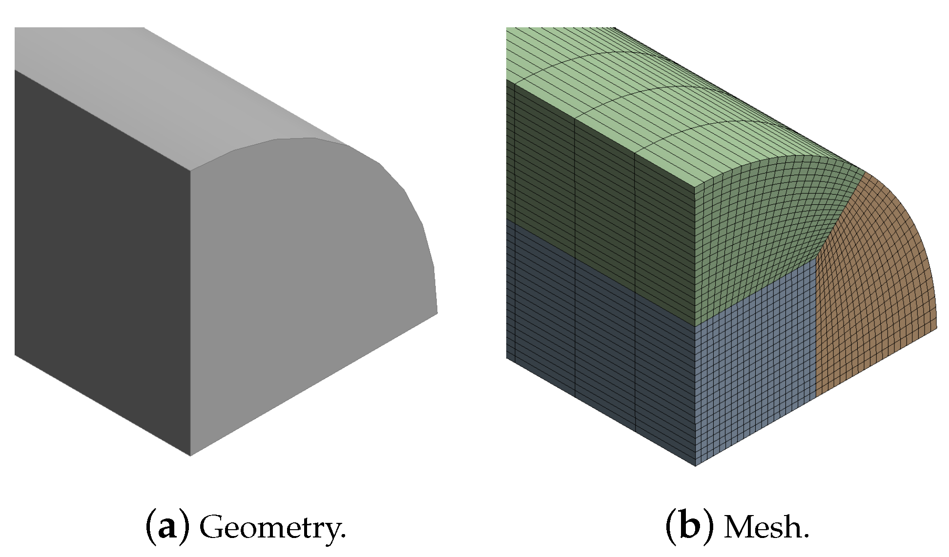
Due to the symmetry of the circular pipeline, a quarter of the fluid domain in the pipeline is established in the CFX software to save computing resources, as shown in Figure 4a. The inner diameter D and length L of the pipeline are set as 4 mm and 2 m, respectively, indicating that it is a significant slender pipeline. In order to obtain better mesh quality, the fluid domain is divided into three regions containing a cuboid with a square bottom for mesh generation, as shown in Figure 4b. For the three regions on the end face, each edge or curve is divided into 20 equal parts. In addition, the model is divided into 4000 equal parts along the axial direction to reduce the aspect ratio of the elements and so as to improve the quality. Then, the number of generated hexahedral elements and nodes are 4,800,000 and 5,045,261, respectively.

The fluid is set as a 22# hydraulic oil, whose kinematic viscosity is 22cSt at a standard atmospheric pressure and a working temperature of 40 °C. Its density is set as 850 kg/m${}^3$. Then, its initial dynamic viscosity ${\eta }_0$ is $22\mathrm{cSt}\times 850\mathrm{kg}/{\mathrm{m}}^3=0.0187\mathrm{Pa}·\mathrm{s}$.

A user-defined expression is created to import the viscosity–pressure characteristics expressed by Equation (2). For hydraulic oils, the viscosity–pressure index $\alpha$ is within $1.5\times {10}^{-8}$ Pa${}^{-1}$ to $3.5\times {10}^{-8}$ Pa${}^{-1}$ [27,29,30]. In this CFD model, set $\alpha$ as $2.2\times {10}^{-8}$ Pa${}^{-1}$, which is the viscosity-pressure index of the HFD fire-resistant hydraulic oil [30].

The flow rate Q is set as 5 L/min, and its equivalent mass flow rate is

$$5\mathrm{L}/\min \times 850\mathrm{kg}/{\mathrm{m}}^3=0.07083333\mathrm{kg}·\mathrm{s}.$$

Then, the inlet of the fluid domain is set as a mass flow rate inlet with one-quarter of the calculated mass flow rate since it is a quarter model. The ambient pressure at the bottom of the Mariana Trench is about 110 MPa, and, if the load pressure is 15 MPa, the outlet pressure $p_o$ of the fluid domain is set as 125 MPa. The cut plane and the cylindrical surface are set as the symmetry boundary and the wall boundary, respectively.

According to the aforementioned parameter settings and the hydraulic oil viscosity of 125 MPa at the outlet of the pipeline, the Reynolds number is 77.08, indicating laminar flow. Then, the analysis type is set as steady-state and the turbulence type is set as none, which means laminar flow. The minimum and maximum iterations are 50 and 100, respectively. The convergence criteria is an RMS (Root Mean Square) type residual with a target value of $1\times {10}^{-4}$.

To improve the precision and reliability of the simulation results, a mesh independence study was conducted based on the aforementioned simulation settings.

Table 1. Sets of mesh elements.

Case	1	2	3	4	5	6
Number of mesh elements	300,000	1,200,000	2,025,000	4,800,000	5,808,000	7,500,000

lists the number of total mesh elements in six cases. How the pipeline pressure loss, the average flow velocity at the outlet, and the calculation time change with the number of elements are shown in Figure 5. According to Table 1 and Figure 5, the pressure loss and the average flow velocity can be considered stable when the number of mesh elements exceeds 4,800,000. The calculation time increases with the number of mesh elements and is about 1200 s or about 20 min in the case with 4,800,000 elements. Therefore, the CFD simulation of a model with 4,800,000 elements has satisfied calculation accuracy and fast calculation speed at the same time.

Based on the established CFD model, the pipeline flow simulation of the deep-sea hydraulic system is carried out. At the same time, a simulation that does not consider the change in hydraulic oil viscosity, which is based on Equation (3), is also carried out for comparison.

4. CFD Results

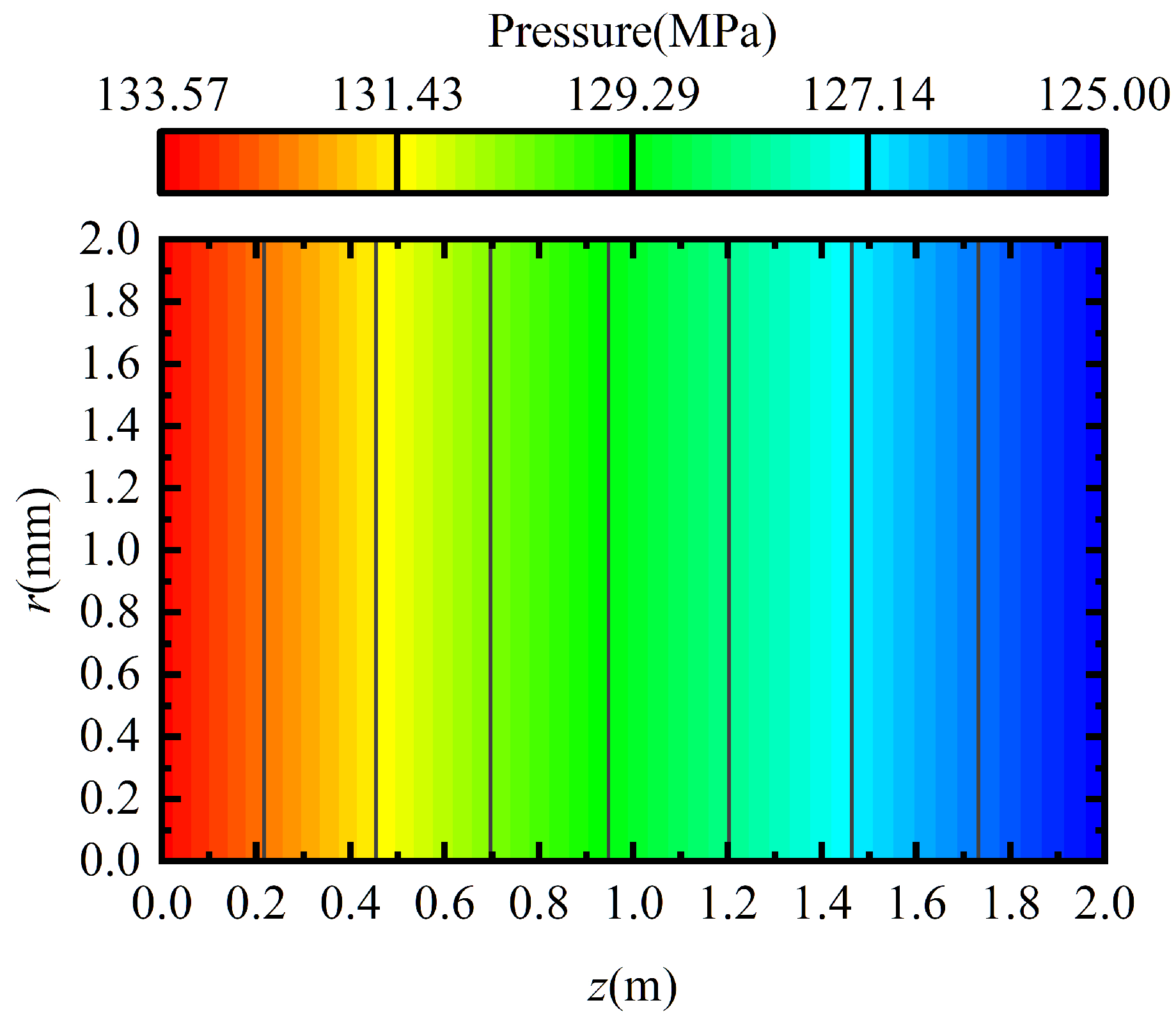
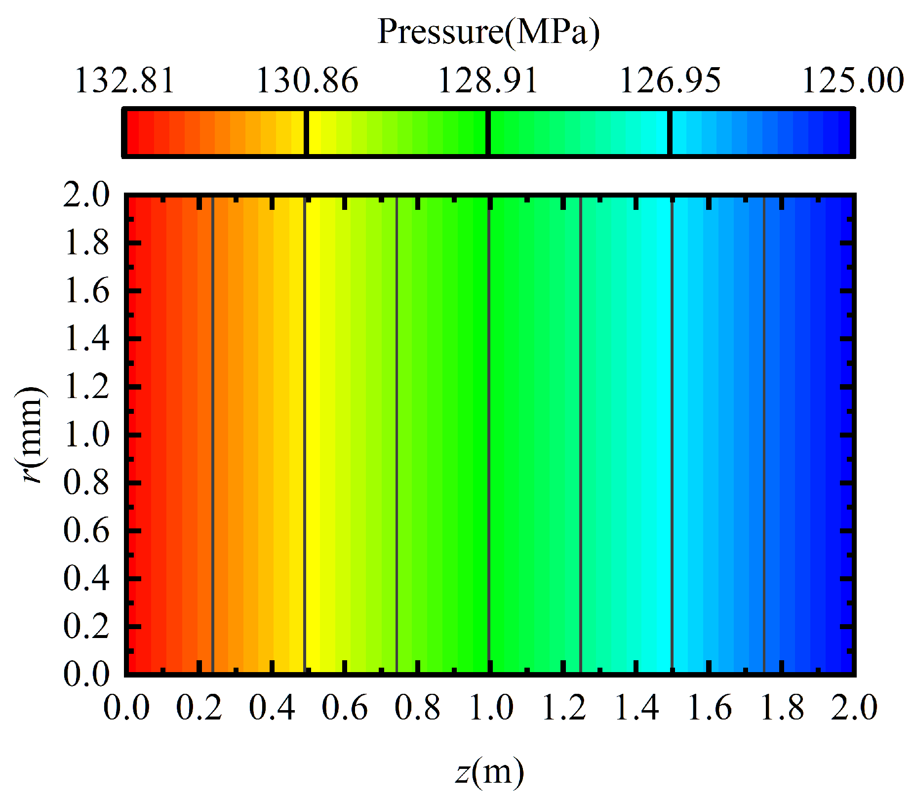
Dynamic viscosity, pressure distribution with variable viscosity, and pressure distribution with constant viscosity are shown in Figure 6, Figure 7 and Figure 8, respectively. Figure 6 shows that the established CFD successfully takes into account the viscosity change during the flow process. Calculated with the viscosities of the inlet and outlet in Figure 6, the viscosity of the hydraulic oil changes by 20.79% when flowing through the pipeline. Comparing Figure 7 and Figure 8, it can be known that the pressure loss considering the viscosity change during the flow process is greater than in the case where the viscosity is constant.

The simulated pressure loss can be obtained by reading the average value of the inlet pressure and subtracting the set outlet pressure of 125 MPa from it, as shown in

Table 2. Pressure loss.

	Simulated Value	Theoretical Value	Error
Pressure loss with variable viscosity	8.53858 MPa	8.50808 MPa	−0.36%
Pressure loss with constant viscosity	7.78795 MPa	7.75926 Mpa	−0.37%
Increment percentage	9.64%	9.65%	-

. The theoretical values calculated according to Equations (3) and (23) are also listed.

From the data in Table 2, it can be known that the theoretical results are in good agreement with the simulation results. According to the setting in Section 3, the load pressure is 15 MPa. Therefore, it can be calculated that the load capacity has dropped by 39.64%, which indicates that the operating performance of the deep-sea hydraulic system is greatly affected. In addition, the pressure loss that takes the viscosity change into account is 9.6% larger than the pressure loss in which the viscosity is constant. This means, in the deep-sea environment, the viscosity change during the flow process in the pipeline has a significant impact on the pipeline pressure loss.

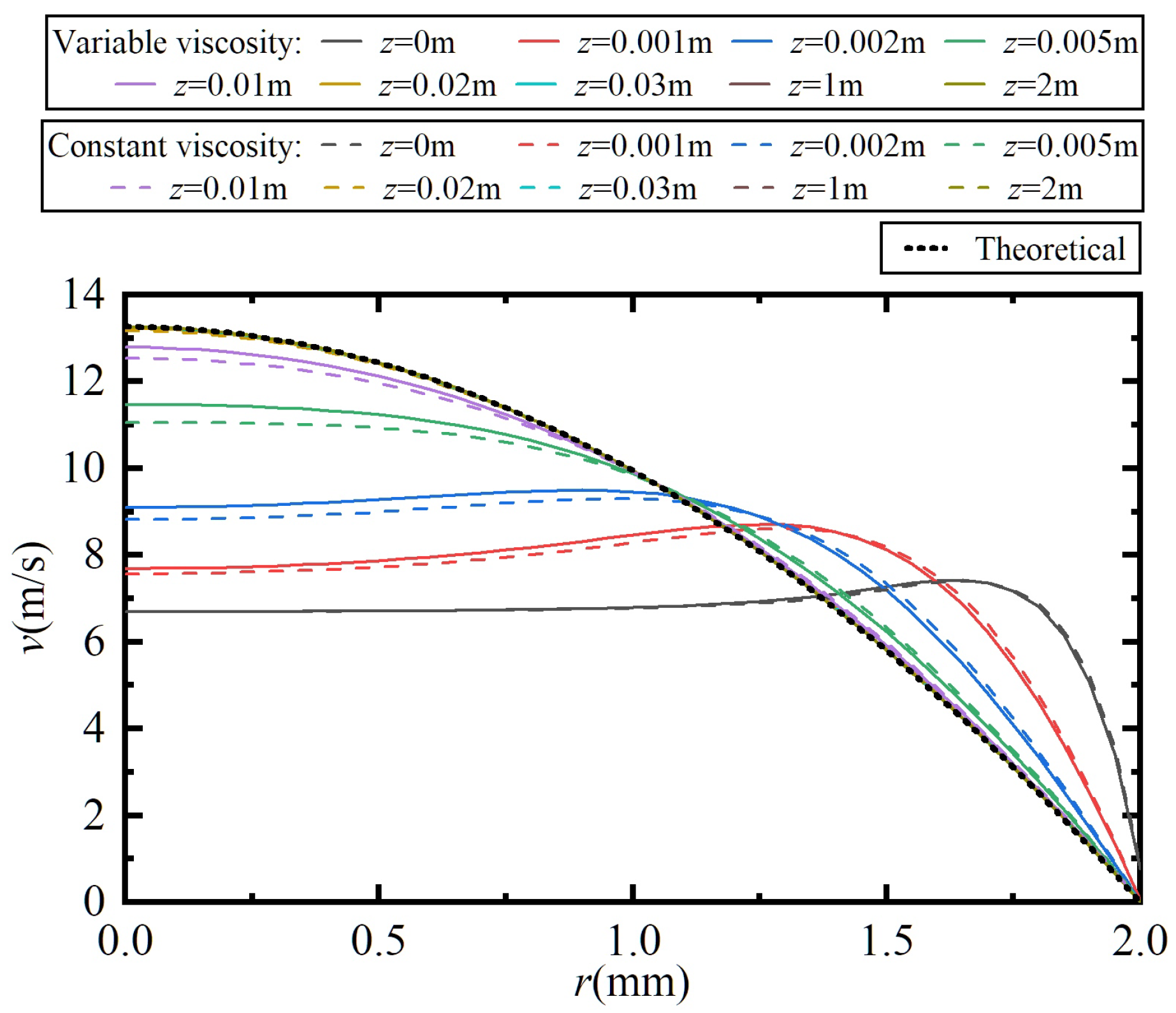
The flow velocity distribution is shown in Figure 9, in which the theoretical distribution curve according to Equation (22) is also plotted. Figure 9 shows that, regardless of whether the viscosity change during the flow process is considered, the flow velocity distribution is in good agreement with each other, which is consistent with the theoretical analysis in Section 2. The velocity distribution at the inlet or at a position less than 0.01 m away from the inlet is quite different from the theoretical distribution. This is caused by the uniform input of fluid at the flow inlet with an average flow velocity. The difference only exists in positions less than 0.01 m away from the inlet, whose range is extremely low compared to the pipeline length of 2 m. As for a position more than 0.01 m away from the inlet, the velocity distribution is in good agreement with the theoretical distribution.

In order to more comprehensively verify the proposed novel equation for pipeline pressure loss expressed by Equation (23), more CFD simulation calculations with variable input parameters are carried out, whose inputs and pressure losses are all listed in

Table 3. Variable inputs and pressure losses: part A.

Parameter	Symbol	Unit	Case 1	Case 2	Case 3	Case 4	Case 5	Case 6	Case 7
Viscosity-pressure index	$\alpha$	Pa${}^{-1}$	$2.2\times {10}^{-8}$	$1.5\times {10}^{-8}$	$2.5\times {10}^{-8}$	$2.2\times {10}^{-8}$	$2.2\times {10}^{-8}$	$2.2\times {10}^{-8}$	$2.2\times {10}^{-8}$
Initial kinematic viscosity	-	cSt	22	22	22	32	46	22	22
Pipeline length	L	m	2	2	2	2	2	1.5	2.5
Pipeline inner diameter	D	mm	4	4	4	4	4	4	4
Outlet pressure of the pipeline	$p_o$	MPa	125	125	125	125	125	125	125
Flow rate	Q	L/min	5	5	5	5	5	5	5
Reynolds number	-	-	77.08	184.90	52.98	52.99	32.86	77.08	77.08
Simulated pressure loss	$\Delta p$	MPa	8.53858	3.34203	13.29610	13.00440	20.10700	6.26105	10.93880
Theoretical pressure loss	$\Delta p$	MPa	8.50808	3.31564	13.26488	12.97332	20.06797	6.22717	10.90953
Error	-	-	−0.36%	−0.79%	−0.23%	−0.24%	−0.19%	−0.54%	−0.27%

and

Table 4. Variable inputs and pressure losses: part B.

Parameter	Symbol	Unit	Case 1	Case 2	Case 3	Case 4	Case 5	Case 6
Viscosity-pressure index	$\alpha$	Pa${}^{-1}$	$2.2\times {10}^{-8}$	$1.5\times {10}^{-8}$	$2.5\times {10}^{-8}$	$2.2\times {10}^{-8}$	$2.2\times {10}^{-8}$	$2.2\times {10}^{-8}$
Initial kinematic viscosity	-	cSt	22	22	22	22	22	22
Pipeline length	L	m	2	2	2	2	2	2
Pipeline inner diameter	D	mm	6	8	4	4	4	4
Outlet pressure of the pipeline	$p_o$	MPa	125	125	85	45	125	125
Flow rate	Q	L/min	5	5	5	5	4	6
Reynolds number	-	-	51.39	38.54	185.83	448.02	61.66	92.49
Simulated pressure loss	$\Delta p$	MPa	1.56294	0.48855	3.36462	1.37981	6.69430	10.46120
Theoretical pressure loss	$\Delta p$	MPa	1.55913	0.48756	3.33803	1.35494	6.67429	10.41898
Error	-	-	−0.24%	−0.20%	−0.79%	−1.80%	−0.30%	−0.40%

. According to the data in Table 3 and Table 4, all simulated pressure losses are in good agreement with the theoretical pressure losses calculated by Equation (23), and the maximum error is −1.80%. All the CFD results justify the correctness of the proposed novel equation for pipeline pressure loss in this paper.

5. Discussions

The CFD calculation results in the last section fully prove the correctness of the proposed novel equation for pipeline pressure loss. In this section, this novel equation will be further analyzed and discussed.

According to Equation (23), the pressure loss considering variable viscosity is related to hydraulic oil properties, pipeline dimensions, and working conditions. Because the expression contains logarithmic and exponential operations, it becomes difficult to directly analyze the relationship between pressure loss and various parameters. Therefore, based on Equation (23) and the set values in Section 3, curves are drawn to show how the pressure loss varies with each parameter. In addition, the increment percentage of pressure loss compared to classical Poiseuille’s law, which can be calculated with Equations (3) and (23), is plotted. In addition, so is the change percentage of viscosity calculated by Equation (4).

5.1. Influence of Hydraulic Oil Properties

It can be known from Figure 10 and Figure 11 that the pressure loss increases with the increase in the viscosity-pressure index or the initial viscosity. The greater the viscosity index is, the faster the pressure loss increases, while the pressure loss changes approximately linearly with the initial viscosity. The increment percentage of pressure loss compared to classical Poiseuille’s law and the change percentage of viscosity show a similar pattern of change.

According to the pressure loss changes shown in Figure 10 and Figure 11, for deep-sea hydraulic systems, it is recommended to use hydraulic oil with a low viscosity-pressure index and a low initial viscosity, which can reduce pipeline pressure loss, thereby improving work efficiency and load capacity. In addition, comparing Figure 10 and Figure 11, it can be known that the viscosity-pressure index has a greater impact on pressure loss, so hydraulic oils with a low viscosity-pressure index should be given priority.

According to the percentage curves in Figure 10 and Figure 11, it can be known that, when the viscosity of the hydraulic oil flowing through the pipeline changes minimally, the pressure loss calculated by Equation (23) is less different from the classic Poiseuille’s law. When the viscosity changes greatly, the difference between the two calculation methods becomes larger. According to Figure 10, when the viscosity-pressure index is $3\times {10}^{-8}$ Pa${}^{-1}$, the viscosity changes by 172.30%, and the difference in pressure loss calculated by the two methods reaches 58.31%.

5.2. Influence of Pipeline Dimensions

According to Figure 12, the pressure loss increases approximately linearly with the increase in the pipeline length, and so do the two percentage curves. As for the influence of pipeline inner diameter that is shown in Figure 13, the pressure loss decreases sharply as the pipeline inner diameter increases when the pipeline inner diameter is less than 12 mm. When the pipeline inner diameter is greater than 12 mm, the pressure loss changes minimally. The two percentage curves in Figure 13 also show a similar pattern of change.

Then, for deep-sea hydraulic systems, it is recommended to use pipelines with short lengths and large inner diameters to reduce pipeline pressure loss, thereby improving work efficiency and load capacity. In addition, according to Figure 13, an excessively large pipeline inner diameter contributes minimally to reducing pipeline pressure loss but increases the weight and space of the deep-sea hydraulic system.

The percentage curves in Figure 12 and Figure 13 also indicate that, when the viscosity of the hydraulic oil changes minimally, the pressure loss calculated by Equation (23) is less different from the classic Poiseuille’s law.

5.3. Influence of Working Conditions

The maximum outlet pressure of 140 MPa in Figure 14 is obtained from the ambient pressure of 110 MPa at the bottom of the Mariana Trench plus the load pressure of 30 MPa. It can be known from Figure 14 and Figure 15 that the pressure loss increases with the increase in the outlet pressure or the flow rate. The greater the outlet pressure is, the faster the pressure loss increases, while the pressure loss changes approximately linearly with the flow rate. The percentage curves show a similar pattern of change.

According to Figure 14 and Figure 15, for deep-sea hydraulic systems, attention should be paid to the working conditions of large working flow rate or large pipeline outlet pressure, in which large pipeline pressure loss would occur and, thereby, reduce the work efficiency and load capacity of the deep-sea hydraulic system. Besides, by comparing Figure 14 and Figure 15, it can be known that the pipeline outlet pressure has a greater impact on pressure loss. For the inflow pipeline which connects the hydraulic pump and the hydraulic actuator, the pipeline outlet pressure is the sum of the load pressure and the ambient pressure in the deep sea. As for the return pipeline that connects the hydraulic actuator and the oil tank, pipeline outlet pressure equals ambient pressure. Then, it can be known that the extremely high ambient pressure in the deep-sea environment has a significant impact on the working efficiency and load capacity of the deep-sea hydraulic system.

The percentage curves in Figure 14 and Figure 15 also indicate that, when the viscosity of the hydraulic oil changes minimally, the pressure loss calculated by Equation (23) is less different from the classic Poiseuille’s law.

The temperature also has a great influence on the viscosity of hydraulic oil. However, because the hydraulic system has a large number of heat sources, and the low-temperature seawater with a large specific heat capacity is sufficient, the thermal field distribution of deep-sea hydraulic pipelines becomes very complicated. Therefore, the influence of temperature is not considered in the theoretical analysis and CFD simulation in this paper, and it is assumed that the hydraulic system is operating at a design condition of 40 °C. The following only briefly discusses the influence of temperature.

The viscosity of hydraulic oil increases greatly in low-temperature conditions. Due to sufficient seawater with a large specific heat capacity and low temperature, the heat dissipation conditions of deep-sea hydraulic systems are much better than those in land conditions. When the deep-sea hydraulic system has not been started or is in a standby state for a long time, the temperature of the hydraulic oil will tend to be the same as the seawater temperature, which is only about 2–4 °C. As a result, the viscosity of hydraulic oil greatly increases. This can significantly increase the pipeline pressure loss when the deep-sea hydraulic system is cold started or restored from a long-term standby state compared with the normal working state. Therefore, the work efficiency and the load capacity of deep-sea hydraulic systems are greatly reduced.

5.4. Relationship between the Novel Equation and the Classic Poiseuille’s Law

According to the discussions in the previous subsections, when the pressure loss or the viscosity change is minimal, the pressure loss calculated by Equation (23) is almost the same as the result of the classic Poiseuille’s law. In this subsection, the relationship between them will be discussed from the perspective of theoretical analysis.

The transformation of Equation (23), which is the proposed novel equation for pipeline pressure loss, is as follows

$$-\alpha \Delta p=ln(1-\frac{128\alpha {\eta }_{0}LQ{e}^{\alpha p_o}}{\pi D^4}).$$

(24)

Taking the natural logarithm of Equation (24), we have

$$e^{-\alpha \Delta p}=1-\frac{128\alpha {\eta }_{0}LQ{e}^{\alpha p_o}}{\pi D^4}.$$

(25)

According to Equations (2) and (4), the term $e^{-\alpha \Delta p}$ indicates the degree of change in hydraulic oil viscosity. When the pressure loss $\Delta p$ is tiny or the viscosity changes minimally, we have

$$e^{-\alpha \Delta p}\approx 1-\alpha \Delta p.$$

(26)

Substituting Equation (26) into Equation (25), we have

$$1-\alpha \Delta p\approx 1-\frac{128\alpha {\eta }_{0}LQ{e}^{\alpha p_o}}{\pi D^4},$$

(27)

or

$$\Delta p\approx \frac{128{\eta }_{0}LQ{e}^{\alpha p_o}}{\pi D^4}.$$

(28)

The expression of Equation (28) is exactly the same as that of Equation (3), which is obtained based on classical Poiseuille’s law.

In addition, the proposed novel equation can be expanded by the Taylor series. The Taylor series of the logarithmic function is

$$ln(1+x)=x-\frac{x^2}{2}+\frac{x^3}{3}-\cdots .$$

(29)

Then,

$$\begin{array}{c}\Delta p=-\frac{1}{\alpha }ln(1-\frac{128\alpha {\eta }_{0}LQ{e}^{\alpha p_o}}{\pi D^4})\hfill \\ =-\frac{1}{\alpha }ln\left[1+\left(-\frac{128\alpha {\eta }_{0}LQ{e}^{\alpha p_o}}{\pi D^4}\right)\right]\hfill \\ =-\frac{1}{\alpha }\left[\left(-\frac{128\alpha {\eta }_{0}LQ{e}^{\alpha p_o}}{\pi D^4}\right)-\frac{{\left(-\frac{128\alpha {\eta }_{0}LQ{e}^{\alpha p_o}}{\pi D^4}\right)}^2}{2}+\frac{{\left(-\frac{128\alpha {\eta }_{0}LQ{e}^{\alpha p_o}}{\pi D^4}\right)}^3}{3}-\cdots \right]\hfill \\ =\frac{128{\eta }_{0}LQ{e}^{\alpha p_o}}{\pi D^4}+\frac{1}{\alpha }\frac{{\left(-\frac{128\alpha {\eta }_{0}LQ{e}^{\alpha p_o}}{\pi D^4}\right)}^2}{2}-\frac{1}{\alpha }\frac{{\left(-\frac{128\alpha {\eta }_{0}LQ{e}^{\alpha p_o}}{\pi D^4}\right)}^3}{3}+\frac{1}{\alpha }\times \cdots .\hfill \end{array}$$

(30)

The first term in Equation (30) is a one-time term, which is also exactly the same as Equation (3).

The derivation of the above two methods shows that the proposed novel equation for the pipeline pressure loss is equivalent to the classic Poiseuille’s law when the pipeline pressure loss or the viscosity change is minimal. Then, we can conclude that the classic Poiseuille’s law is a simplified expression of the novel proposed equation for pipeline pressure loss in the case of small viscosity changes. In other words, the novel pressure loss equation is an extension of the classic Poiseuille’s law.

6. Conclusions

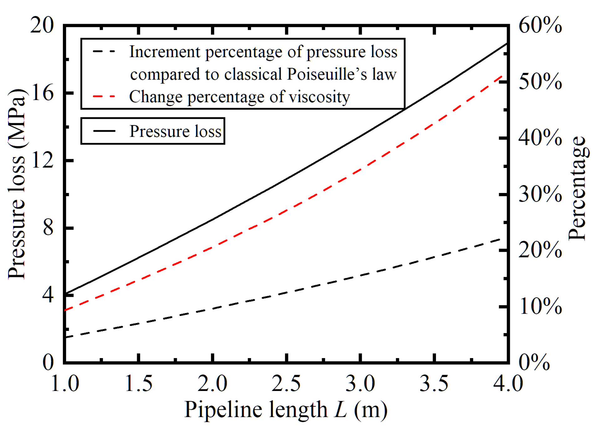
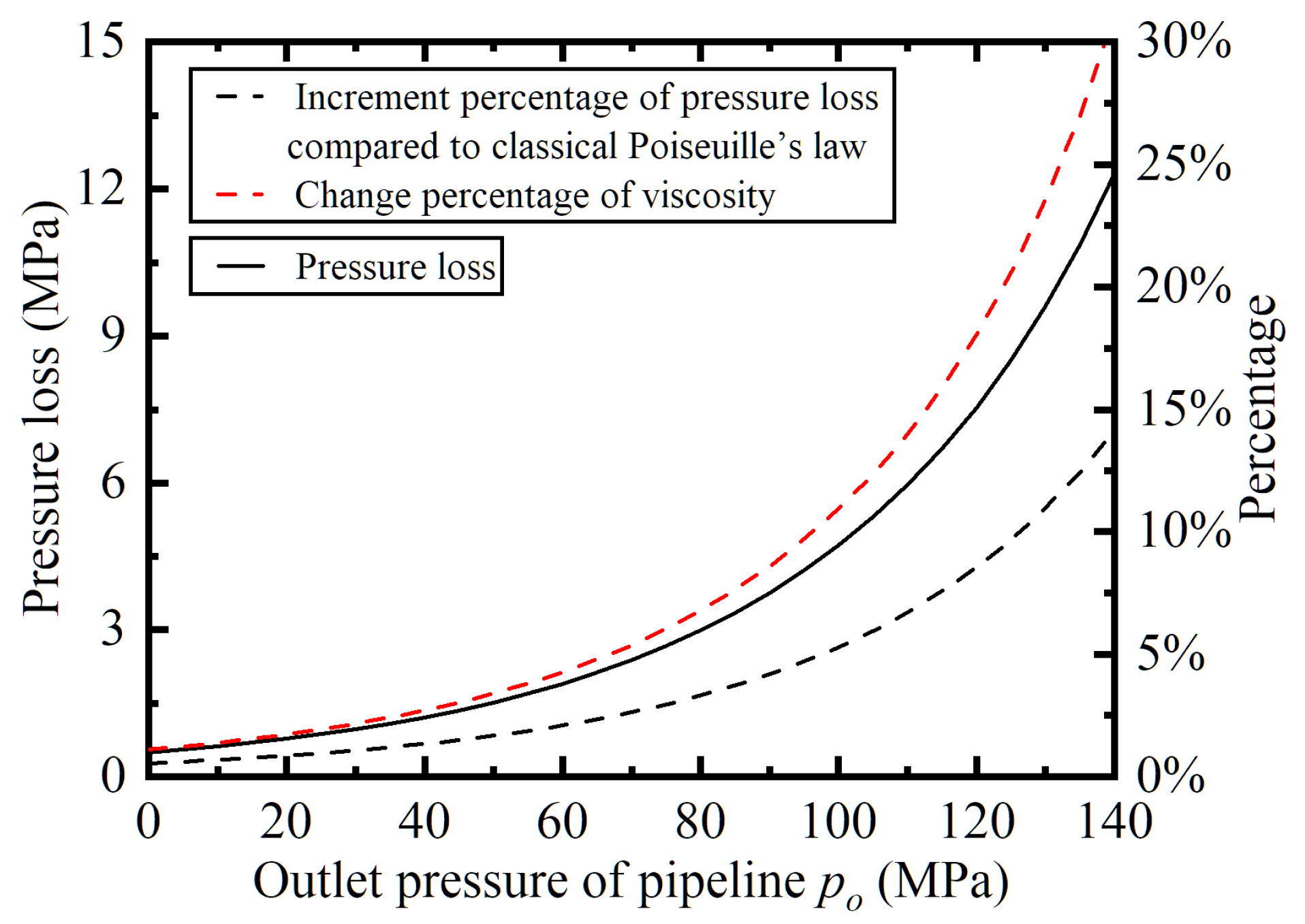
(1.) Based on laminar flow theory and the viscosity-pressure characteristics of hydraulic oil, a novel equation for pipeline pressure loss is proposed, in which the viscosity change when flowing through the pipeline is taken into account. The pipeline pressure loss is related to the viscosity-pressure index and the initial viscosity of the hydraulic oil, the length and inner diameter of the pipeline, the flow rate, and the outlet pressure.

(2.) Theoretical analysis shows that the proposed novel equation for pipeline pressure loss is equivalent to the classic Poiseuille’s law when the pipeline pressure loss or the viscosity change is minimal, which means the novel pressure loss equation is an extension of the classic Poiseuille’s law.

(3.) The larger the viscosity-pressure index or the initial viscosity of the hydraulic oil, the length of the pipeline, the flow rate, or the outlet pressure is, the greater the deviation between the pressure loss calculated by the proposed novel equation and the classic Poiseuille’s law. In addition, the smaller the inner diameter of the pipeline is, the greater the deviation is. The difference in pressure loss calculated by the two methods reaches 58.31% when the viscosity-pressure index of the hydraulic oil is $3\times {10}^{-8}$ Pa${}^{-1}$.

(4.) A CFD model of a pipeline in the deep-sea hydraulic system is established, and CFD simulations are conducted. The maximum error between the pressure loss calculated by the novel equation and the one calculated by the CFD simulation is only −1.80%. The fluid velocity distribution obtained by CFD simulation is consistent with the theoretical analysis. All the CFD results justify the correctness of the proposed novel equation for pipeline pressure loss.