Fishing Net Health State Estimation Using Underwater Imaging

Abstract

Fishing net cleanliness plays a critical role for aquaculture industry as bio-fouled nets restrict the flow of water through the net leading to a build-up of toxins and reduced oxygen levels within the pen, thereby putting the fish under increased stress. In this paper, we proposed an underwater fishing Net Health State Estimation (NHSE) method, which can automatically analyze the degree of fouling on the net through underwater image analysis using remotely operated vehicles (ROV) images, and calculate a blocking percentage metric of each net opening. The level of fouling estimated through this method help the operators decide on the need of cleaning or maintenance schedule. There are mainly six modules in the proposed NHSE method, namely user interaction, distortion correction, underwater image dehazing, marine growth segmentation, net-opening structure analysis, and blocked percentage estimation. To evaluate the proposed NHSE method, we collected and labeled several underwater images in Mulroy Bay, Ireland with pixel-wise annotations. In order to verify the universality and robustness of the algorithm, we simulated and built a virtual fishing farm, and, on this basis, collected and labeled fishing net images under different environmental conditions. Seven evaluation metrics are introduced to demonstrate the effectiveness and advantages of the proposed method.

1. Introduction

Developing new cage farming technologies is important for sustainable and economical aquaculture, while fishing net, which is an integral part of cage, plays an essential role in aquaculture. Generally, there are two ways for cleaning of the fishing net in traditional aquaculture. One way is manually checking the health state of fishing net combined with considering season, temperature and water quality, or cleaning at regular intervals, for instance two weeks in summer. It requires a significant of manpower and material resources whether it is checking or cleaning. Moreover, frequent cleaning will also reduce the overall life-cycle of fishing net.

Hence, a net health state monitoring or estimation technic is of great practical value. Some researchers [1,2,3] focus on designing a monitoring system through different types of sensors, such as water flow sensor, oxygen sensor, or temperature sensor, for combined analyses and subsequent establishment of the current state of the underwater surroundings of fishing net. A multi-sensor based system can get accurate data from different contexts, but the sensor deployment, data collection, and comprehensive analysis still make such systems complex. In this paper, we aim to estimate the health state of fishing net through a more intuitive way, by quantifying visual inspection under water, images are used for fishing net health state estimation, which is more consistent with the way aquaculture professionals obtain standard information.

This study aims to address fishing net health estimation problem by an image processing way, so here we talk about the traditional fishing related environment monitoring and related image processing algorithms. For sensor based monitoring, how to remove the noise of the collected data and comprehensively analyze the multi-sensor data are the keys to this type of algorithm. Cordova-Rozas et al. [2] chose pH and temperature sensors to monitor the water quality and provide real-time information to fish-farmers to anticipate risks and have a more efficient production. In [4], a so-called fish pond monitoring system is designed to collect temperature information without analysis. Wahjuni et al. [3] aim to control some cultivation environment parameters such as pH, dissolved oxygen, and temperature, then design a fuzzy inference system for water quality monitoring. Chen et al. [1] establish an automated monitoring system of wireless sensor networks for fish farm aquaculture environment, which collects temperature, dissolved oxygen, pH, and water level information.

Underwater image processing, limited by marine growth, light, water quality, and seasonal influences, is more challenging than general image processing. Luo et al. [5] proposed a tuna recognition algorithm for fisheries monitoring, which consists of SIFT feature extract and SVM classification. Huang et al. [6] proposed a fish tracking and segmentation algorithm for stereo video-based monitoring on wild sea surfaces. An underwater image enhancement method, which uses minimum information loss and histogram distribution prior, is proposed in [7]. The proposed method includes an underwater image dehazing part and a contrast enhancement part. Christensen et al. [8] presented an optical fish detection network to detect, localize and classify fish in murky water conditions typical of the Baltic and North Sea. Recently, virtual data in subsea inspections [9] and the application of statistical learning algorithms [10] have been observed to be of benefit for detection of features of interest in an underwater environment.

It is observed for aquaculture that most underwater environment monitoring methods are based on multi-sensor data, which collect and combine different types of data for simple analysis and judgement. At the same time, most underwater image processing methods focus on image restoration, enhancement, fish detection, tracking, and classification. Under such circumstances, using images for monitoring, the health of fish nets can be of benefit. This paper proposed a visual information based underwater fishing net health state estimation algorithm and addressed the proposed problem in a number of ways. In particular:

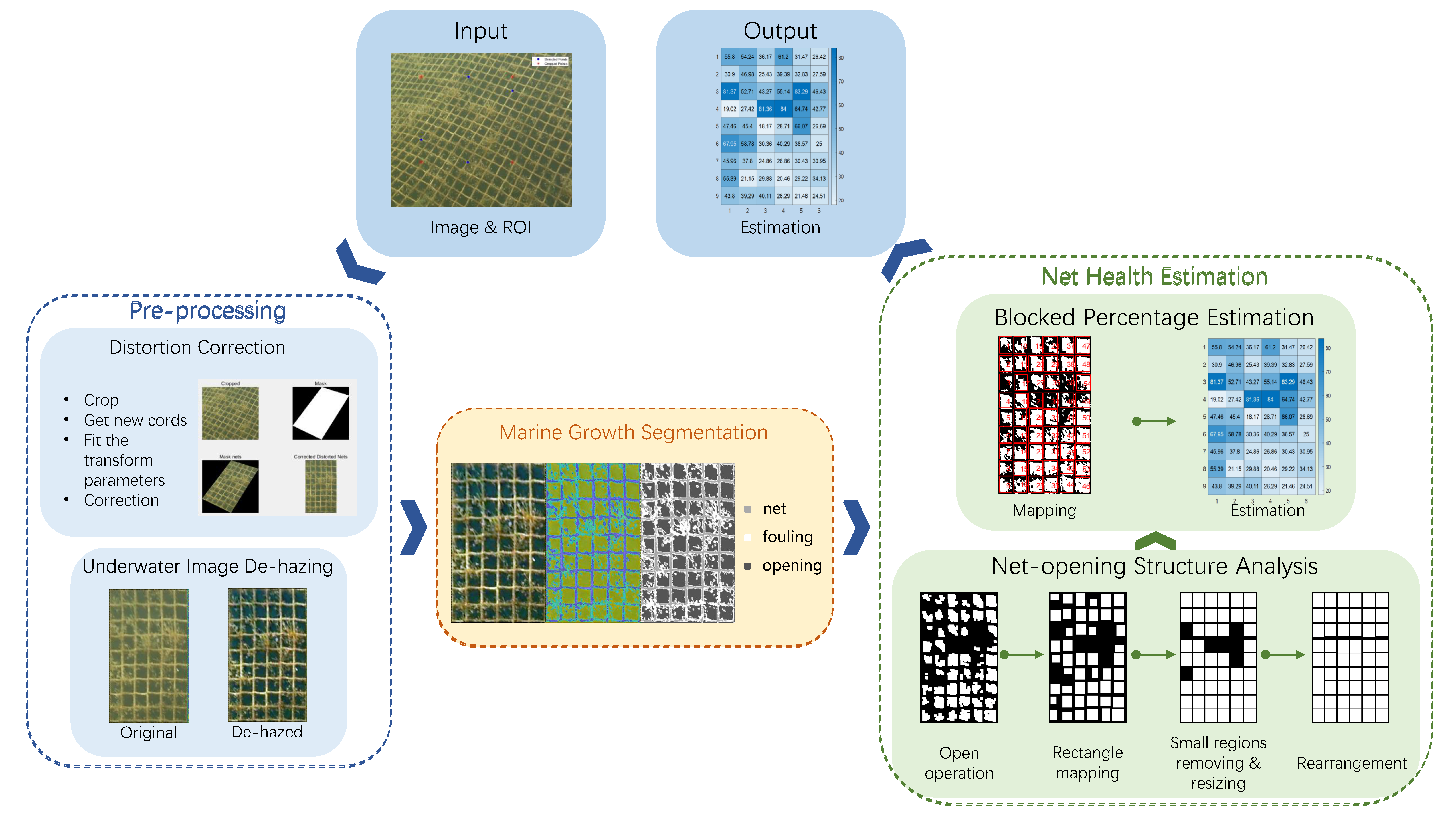
• A visual information based framework of underwater fishing net health state estimation is proposed.
• Net-opening structure analysis and blocked percentage estimation methods are introduced to infer the health state of each net cell.
• A Virtual Fishing Net(VFN) dataset is built, which can easily simulate the situation of fishing nets in different conditions.
• Seven evaluation metrics are introduced for a comprehensive evaluation for both intermediate results and final estimation results.

The findings are expected to highlight the possibilities of underwater image processing in aquaculture and lead to several studies. It also highlights the need and methods of creating a framework for the assessment of the health of fishing net health.

2. Methodology

To ensure the universality, stability, and effectiveness of the proposed Net Health State Estimation (NHSE) algorithm, three modules: pre-processing, marine growth segmentation, and net health estimation modules are designed as shown in Figure 1. For any input underwater image, Region of Interest (RoI) is selected and corrected for further segmentation. The image de-hazing method [11] is introduced to achieve a more accurate and better visualization. Subsequently, we utilize the k-means algorithm to separate the regions of net, bio-fouling, and net-opening. According to the segmentation results, a net-opening structure analysis method is proposed to calculate the number of cells, which greatly affected the results of estimation. Finally, we take both segmentation and structure into consideration to estimate the blocking percentage of each cell.

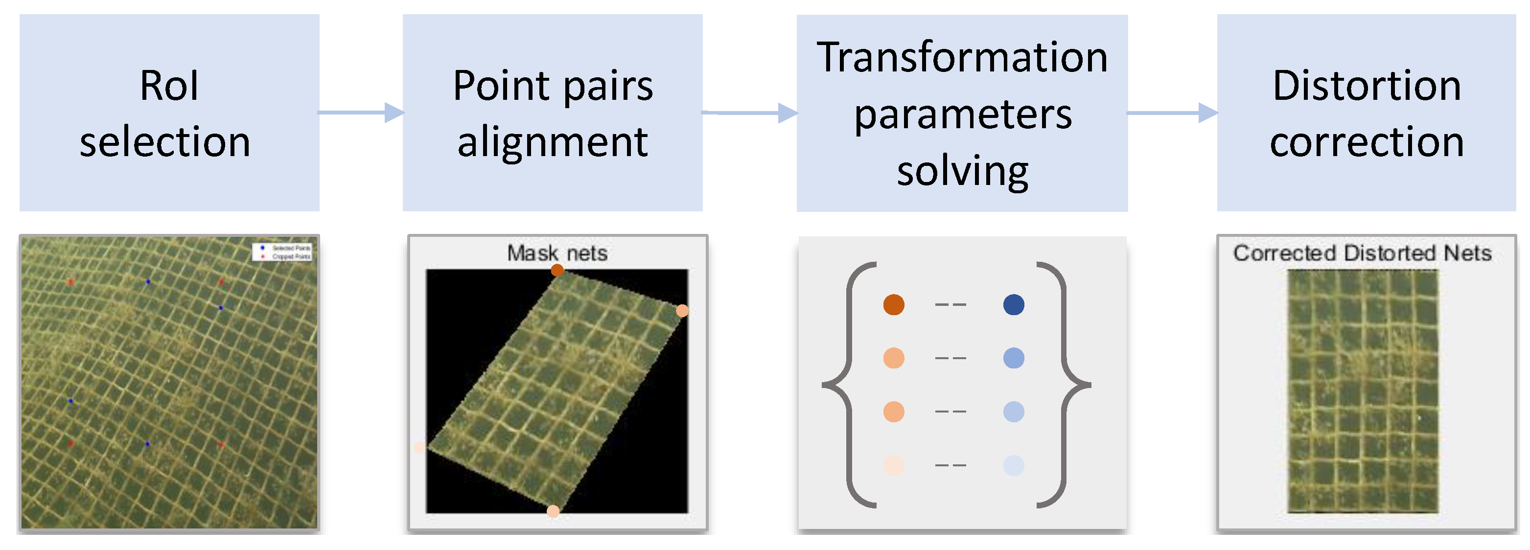
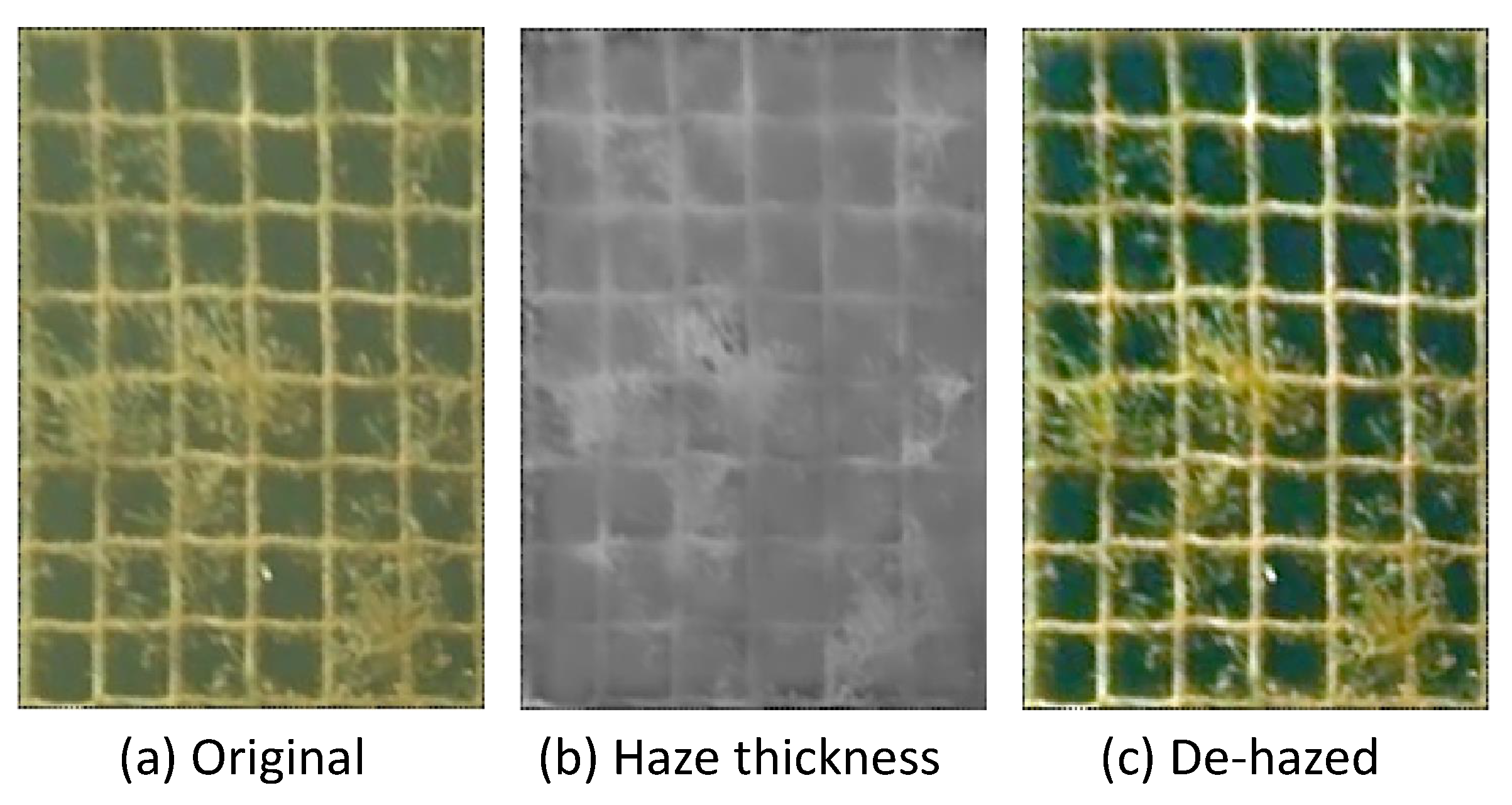
2.1. Pre-Processing

Underwater images captured by ROV have arbitrary angles, scales, and turbidity [12], which increased the difficulty of estimation. Hence, pre-processing, as the first step of NHSE, is necessary to correct and enhance the raw underwater image.

2.1.1. Distortion Correction

Image distortion is mainly caused by five basic operations, namely, translation, scale, flip, rotation, and shear. Simply speaking, affine transformation is a two-dimensional linear transformation, which maintains straightness (transformed straight lines keep straight) and parallelism(parallel lines keep parallel and the order of points in a line remain), includes five aforementioned transformations, and is a composite of them in any combination and sequence, while, for real-world 3D scenes, perspective transformation is more applicable to actual situations. As ROV is working with arbitrary attitude, the collected images have varying types and degrees of distortion. For instance, three common types are illustrated in Figure 2.

In this work, perspective transformation is used for distortion correction as it can cover most situations. Generally speaking, what perspective transformation does is mapping the points $\left(x,y\right)$ on a two-dimensional plane to a three-dimensional space $\left(X,Y,Z\right)$, and then back to the previous two-dimensional plane $\left(x^{\prime },y^{\prime }\right)$ as follows:

$$\left[\begin{array}{c}X\\ Y\\ Z\end{array}\right]=\left[\begin{array}{ccc}{m}_{11}& m_{12}& m_{13}\\ m_{21}& m_{22}& m_{23}\\ m_{31}& m_{32}& m_{33}\end{array}\right]\left[\begin{array}{c}x\\ y\\ 1\end{array}\right]$$

(1)

$$\begin{array}{c}X=m_{11}·x+m_{12}·y+m_{13}\hfill \\ Y=m_{21}·x+m_{22}·y+m_{23}\hfill \\ Z=m_{31}·x+m_{32}·y+m_{33}\hfill \end{array}$$

(2)

$$\begin{array}{c}{x}^{\prime }=\frac{X}{Z}=\frac{m_{11}·x+m_{12}·y+m_{13}}{m_{31}·x+m_{32}·y+m_{33}}\hfill \\ \\ y^{\prime }=\frac{Y}{Z}=\frac{m_{21}·x+m_{22}·y+m_{23}}{m_{31}·x+m_{32}·y+m_{33}},\hfill \end{array},$$

(3)

where $z=1$ means $\left(x,y\right)$ is in a two-dimensional plane. Divide both numerator and denominator by $m_{33}$ in Equation (3), which can be re-written as:

$$\begin{array}{c}{x}^{\prime }=\frac{X}{Z}=\frac{{m^{\prime }}_{11}·x+{m^{\prime }}_{12}·y+{m^{\prime }}_{13}}{{m^{\prime }}_{31}·x+{m^{\prime }}_{32}·y+1}\hfill \\ \\ y^{\prime }=\frac{Y}{Z}=\frac{{m^{\prime }}_{21}·x+{m^{\prime }}_{22}·y+{m^{\prime }}_{23}}{{m^{\prime }}_{31}·x+{m^{\prime }}_{32}·y+1}\hfill \end{array}.$$

(4)

Thus, there are eight unknowns need to be solved as shown in Equation (4). In other words, we need four pairs of points to fit the perspective transformation in this study. Fortunately, four points are selected to determine RoI and also can be used to solve Equation (4). Figure 3 shows the flowchart of distortion correction. In step 2, point pairs alignment is introduced to calculate the new coordinates in cropped plane C, and then get the coordinates in correction plan according to relative location of selected points in plane C. The transformation parameters will be solved in step 3 by Equation (4).

2.1.2. Underwater Image De-Hazing

Due to the complex imaging environment of the ocean/lake, the underwater image captured by ROV has serious degradation. Color deviation caused by light absorption and blurred details and decreased contrast caused by scattering are two main reasons. Therefore, underwater image enhancement is necessary for further analysis to achieve a more accurate estimation. Light travels similarly in air and water; inspired by the image de-hazing algorithm, we utilize a simple yet effective Dark Channel Prior (DCP) algorithm [11] to remove the underwater haze from a single input image. The widely used model to describe the formation of a haze image is as follows: [13,14]:

$$\mathbf{I}\left(\mathbf{x}\right)=\mathbf{J}\left(\mathbf{x}\right)t\left(\mathbf{x}\right)+\mathbf{A}\left(1-t\left(\mathbf{x}\right)\right),$$

(5)

where $\mathbf{I}$ is the observed intensity, $\mathbf{J}$ is the scene radiance, $\mathbf{A}$ is the global light, and t is the medium transmission describing the portion of the light that is not scattered and reaches the camera. The goal of haze removal is to recover $\mathbf{J}$, $\mathbf{A}$, and t from $\mathbf{I}$. The first term $\mathbf{J}\left(\mathbf{x}\right)t\left(\mathbf{x}\right)$ is called direct attenuation [15], which describes the initial scene and its decay in the medium, for instance air or water. In addition, the second term $\mathbf{A}\left(1-t\left(\mathbf{x}\right)\right)$ is called air-light [16], which is caused by scattered light and leads to color shift. Dark channel prior means at least one color channel of non-sky region has very low intensity at some pixels:

$${\mathbf{J}}^{dark}\left(\mathbf{x}\right)=\underset{c\in \left\{r,g,b\right\}}{min}\left(\underset{\mathbf{y}\in \mathsf{\Omega }\left(\mathbf{x}\right)}{min}\left(J^c\left(\mathbf{y}\right)\right)\right)\to 0,$$

(6)

where c is the color channel, $\mathsf{\Omega }\left(\mathbf{x}\right)$ is a patch centered at $\mathbf{x}$. According to Equation (5) and dark channel prior, the estimated transmission $\tilde{t}$ can be derived as:

$$\tilde{t}\left(\mathbf{x}\right)=1-\omega \underset{c}{min}\left(\underset{y\in \mathsf{\Omega }\left(\mathbf{x}\right)}{min}\left(\frac{I^c\left(\mathbf{y}\right)}{A^c}\right)\right),$$

(7)

where $\mathsf{\Omega }=0.95$ is a constant parameter, while the global light $\mathbf{A}$ is regarded as the highest intensity within a patch. Then, the initial scene $\mathbf{J}$ can be recovered as:

$$\mathbf{J}\left(\mathbf{x}\right)=\frac{\mathbf{I}\left(\mathbf{x}\right)-\mathbf{A}}{max\left(t\left(\mathbf{x}\right),t_0\right)}+\mathbf{A},$$

(8)

where $t_0$ is set to 0.1.

Figure 4 shows an example of underwater image de-hazing. Figure 4b is the estimated haze thickness. The de-hazed image has higher contrast and better visualization (Figure 4a) compared with the original image (Figure 4c).

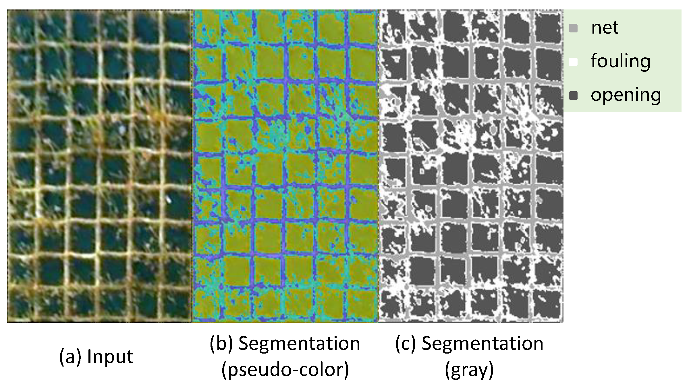
2.2. Marine Growth Segmentation

The corrected and enhanced underwater image is obtained after pre-processing. The goal of this section is to segment out the net-opening regions. Notably, there are totally three kinds of elements: marine growth, fishing net, and net-opening. k-means++ [15], which specifies a procedure to initialize the cluster centers before proceeding with the standard k-means optimization iterations, is introduced for more stable and efficient segmentation. In this work, we initial the number of cluster $k=3$, and segment the image in RGB color space. The main steps of k-means++ are shown in Algorithm 1. The segmentation results are shown in Figure 5.

Algorithm 1 Main steps of k-means++.

1: Choose one center randomly from data   2: For other data point z, compute the distance $D\left(z\right)$ between z and the nearest center   3: Compute the probability $P\left(z\right)$ of being the next center for each point k: $P\left(z\right)=\frac{D{\left(z\right)}^2}{\sum _{z\in \mathrm{Z}}D{\left(z\right)}^2}$   4: Repeat steps 2 and 3 until all k centers are determined   5: Process standard k-means

2.3. Net Health Estimation

The green part as shown in Figure 1, estimating net-opening structure and blocked percentage from the segmentation results are the main tasks of this section. In general, net-opening structure analysis is designed to derive the number, size, and location of each cell, which can be utilized for the blocked percentage estimation part.

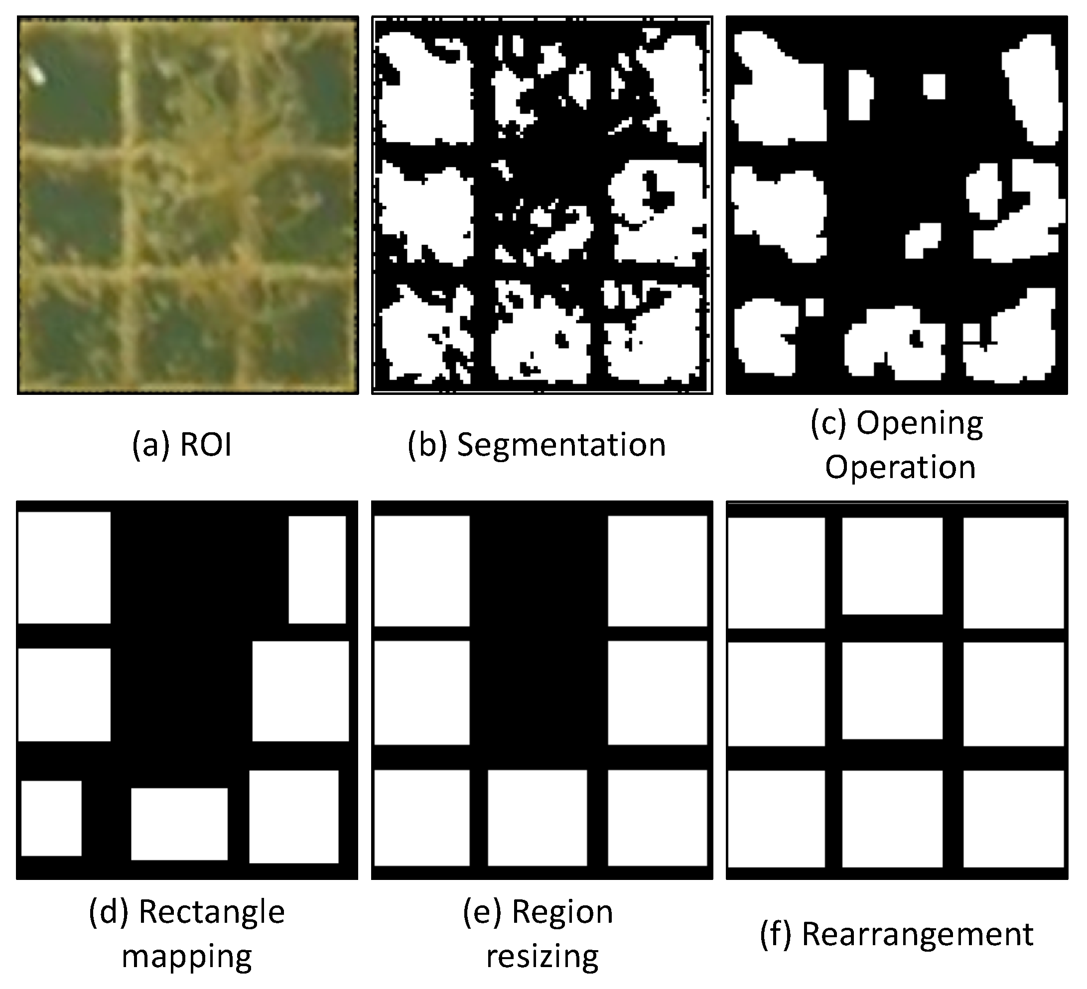
2.3.1. Net-Opening Structure Analysis

The location and size of each cell (i.e., the clean net cell) are critical information for estimation. In this part, the aforementioned information is estimated through the net-opening segmentation results, which, as illustrated in Figure 6, has pixel-wise accuracy due to the de-hazed or enhanced image. However, in the meantime, there are some isolated pixels or small patches, which increased the difficulty in structure analysis.

There are four steps in this part: morphology operation, rectangle mapping, small regions removing and resizing, and rearrangement. Morphology operation is introduced to remove the isolated regions and keep cell regions separated as shown in Figure 6b,c. In this study, we use image opening operation (∘) described as:

$$S\circ B=\left(S\ominus B\right)\oplus B,$$

(9)

where ⊖ and ⊕ denote erosion and dilation, respectively. S is the segmented binary image, while B is the structuring element.

Net-opening areas become more compact and independent to neighbors. Next, remove the small regions and fit the smallest circumscribed rectangle for each net-opening area. Figure 6d shows the mapped rectangle regions; notably, small mapped rectangles can not cover the whole region of a cell. Hence, small regions removing and resizing step aims to replace the incomplete area by an estimated region in the same location. For example, the rectangle in the left corner (in Figure 6d) is replaced by a resized rectangle as shown in Figure 6e.

Here, we define the area of jth $\left(j=1,\dots ,n_j\right)$ region as $R_j$ as shown in Figure 6c, thus, the upper-left and lower-right corners of the initial mapped rectangle ${St}_j$ can determined by $min{\mathbf{X}}_j,min{\mathbf{Y}}_j,max{\mathbf{X}}_j,max{\mathbf{Y}}_j$, where ${\mathbf{X}}_j$ and ${\mathbf{Y}}_j$ are a set of coordinates in jth region. The small regions threshold is set to $0.4\ast R_m$, where $R_m$ is the mean area of all ${St}_j$, the mapped rectangle ${St}_i\in \left\{{St}_j|{St}_j>0.4\ast R_m\right\}$.

As some cells contain more marine growth, the last step can not recover all the missing cells. Step rearrangement is introduced to estimate the center and size of missing cells. In particular, the x- and y-axis coordinates of missing cells are calculated according to the mean column and row coordinate, respectively. In addition, the size of missing cell is estimated as the same way. Now, each cell has a relatively reasonable location and size. The detailed algorithm is shown in Algorithm 2.

Algorithm 2 Region resizing and Rearrangement

Input: $\mathbf{St}=\left\{{St}_i\right\}$ Output: ${\mathbf{St}}^{*}$   1:  the search range: sr;     2:  the centre of i-th rectangle: $C_i=\left(x_i,y_i\right)$;     3:  index of column has maximum number of regions: $MAX\_idx\_col$;     4:  index of row has maximum number of regions: $MAX\_idx\_row$;     5:  initialization;     6:  for ${St}_i$ do     7:      search in column:     8:      $idx\_col=\left\{i|x_i\in \left[max\left(x_i-sr,0\right),min\left(x_i+sr,MAX\_X\right)\right]\right\}$     9:      if $\#idx\_col>\#MAX\_idx\_col$ then    10:          $MAX\_idx\_col\leftarrow idx\_col$    11:      search in row:    12:      $idx\_row=\left\{i|y_i\in \left[max\left(y_i-sr,0\right),min\left(y_i+sr,MAX\_Y\right)\right]\right\}$    13:      if $\#idx\_row>\#MAX\_idx\_row$ then    14:          $MAX\_idx\_row\leftarrow idx\_row$    15:      update $C_i\leftarrow mean\left(C_{idx}\right)$; $H_i\leftarrow mean\left(H_{idx}\right)$; $W_i\leftarrow mean\left(W_{idx}\right)$    16:  for $y_m,m\in \left\{MAX\_idx\_col\right\}$ do    17:      for $x_n,n\in \left\{MAX\_idx\_row\right\}$ do    18:          if $\left(x_i,y_i\right)\notin \left[\left(x_n-sr,y_m-sr\right),\left(x_n+sr,y_m+sr\right)\right]$ then    19:                $W_{mean}\leftarrow \frac{1}{k}{\sum }_{*=1}^{k}W\left(x_{*},y_m\right)$    20:                $H_{mean}\leftarrow \frac{1}{l}{\sum }_{*=1}^{l}H\left(x_n,y_{*}\right)$    21:                create new $St\left\{\left(x_i,y_i\right);W_{mean};H_{mean}\right\}\to {\mathbf{St}}^{*}$    22:  return ${\mathbf{St}}^{*}$

2.3.2. Blocked Percentage Estimation

The structure for each cell $S{t}_i$ is obtained by the net-opening structure analysis module. In addition, the net-opening segmentation results can be treated as the area $O_i$, and then the blocked percentage ${BP}_i$ can be computed simply as:

$${BP}_i=\frac{O_i}{{St}_i}.$$

(10)

3. Experiments

3.1. Dataset

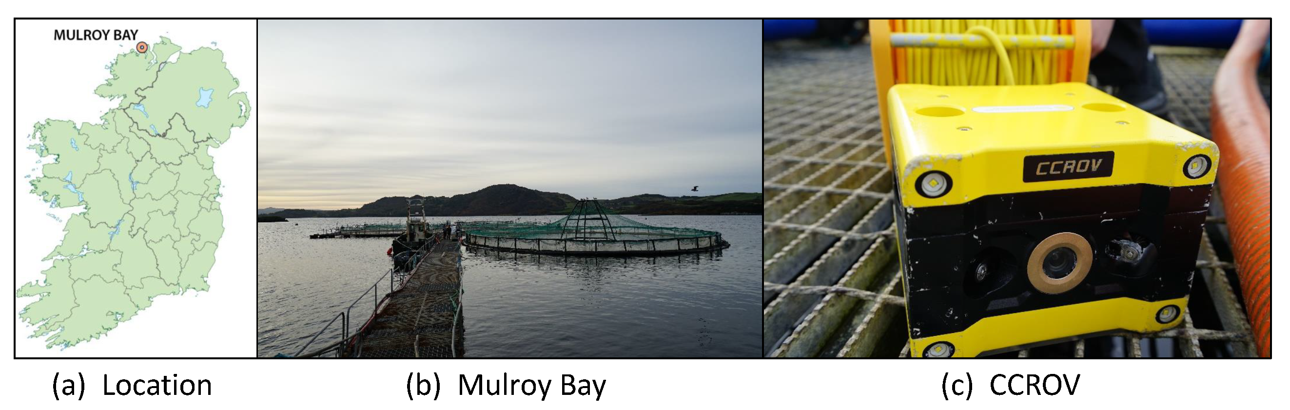
3.1.1. Real Scene Dataset

To the best of the authors’ knowledge, there is no benchmark underwater net blockage percentage estimation dataset. Under such circumstances, we collected and labeled 30 underwater images from five raw underwater images for evaluation. All the raw images are captured by CCROV in Mulroy Bay, Ireland as shown in Figure 7. The detailed camera settings is listed in

Table 1. Camera settings.

Image sensor	Sony IMX 117 1/2.3 inch CMOS
Lens	FOV90°, f/2.8, infinity focus
Image resolution	4000 × 3000
Video resolution	4K (3840 × 2160) 30P

. Such development of varied images from observed data have been done before with extensive investigation of detection performance through receiver operating characteristics [12,17].

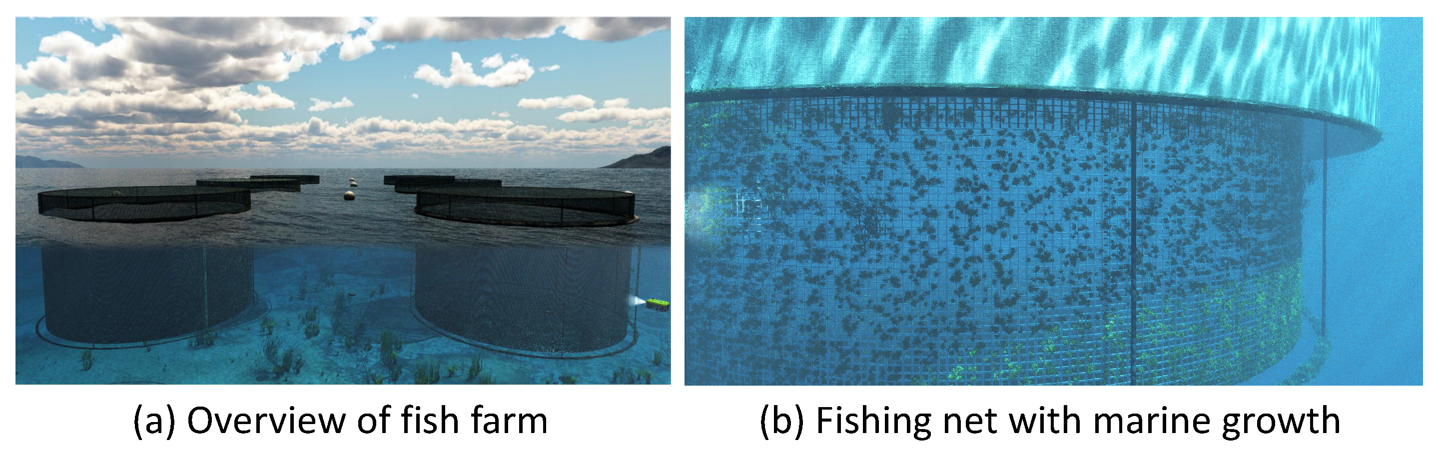
3.1.2. Virtual Fishing Net (VFN) Dataset

As collecting the real scene data are extremely expensive and time-consuming, a customized virtual scene [9] can help us to get enough samples with varied conditions, such as colors of water, angles, densities of marine growth, and visibilities. In this work, VUE xStream is used to build the virtual fishing farm under the guidance of SINTEF Ocean Research Institute combined with our experience on visiting the real site called the Mulroy Bay in Ireland. Figure 8 shows some overview images of the virtual farm.

Six raw virtual scenes are captured and labelled from the built virtual fishing farm. In order to be more in line with the real scenes, different viewing angles, colors, visibilities, and densities of marine growth as shown in Figure 9, are taken into consideration. For each raw scene, 30 samples are then captured manually following the principle of covering most part of the raw image. Figure 10 shows some samples with two kinds of ground truth. The pixel-wise ground truth is generated by labeling the net and marine growth part, while the rectangle ground truth is used to locate the hole of the clean fishing net. Both pixel-wise and rectangle ground truth are combined for evaluation.

3.2. Evaluation Metrics

There are three intermediate results in NHSE: net-opening segmentation, net hole location, and blocked percentage estimation. Thus, here we introduce seven evaluation metrics: precision, recall, F1-score for segmentation results, mean IoU (Intersection-Over-Union), standard deviation of IoU for location results, Pearson Correlation Coefficient(PCC), and mean error for blocked percentage.

3.2.1. For Segmentation Results

Precision, Recall and F1-score are widely used in image segmentation. In this work, the net-opening part segmentation, as the first module, should be evaluated and lay the foundation for health state estimation. Precision and Recall can be calculated simply as:

$$precision=\frac{TP}{TP+FP}$$

(11)

$$recall=\frac{TP}{FN+TP},$$

(12)

where TP, FP, and FN are True Positive, False Positive, and False Negative, respectively. F1-score can be interpreted as a weighted average of the precision and recall, where an F1-score reaches its best value at 1 and worst score at 0. The relative contribution of precision and recall to the F1-score are equal. The formula for the F1-score is:

$$F_1=\frac{2TP}{2TP+FP+FN}.$$

(13)

3.2.2. For Location Results

Intersection over Union (IoU) is an evaluation metric used to measure the accuracy in object detection. In this work, IoU is introduced to evaluate the performance of the Net-opening Structure analysis module as shown in Section 2.3. The mean IoU of all net-opening boxes can therefore be determined via:

$$mIoU=\sum _{i=1}^n\frac{{AO}_i}{{AU}_i},$$

(14)

where n is the total number of net-opening boxes, In the numerator, we compute the area of overlap between the predicted net-opening box and the ground-truth bounding box. While AU is the area encompassed by both the predicted net-opening box and the ground-truth bounding box, stdIoU is simply the standard deviation of all IoU.

3.2.3. For Blocked Percentage Results

There are no ready-made criteria for net health state estimation. The output of the proposed NHSE is a matrix of blocked percentage of each net-opening, while the ground truth of blocked percentage is calculated by the labeled pixel-wise segmentation and rectangle information described in Section 3.1. The goal of evaluation is to measure the differences or relations between two aforementioned matrices. Thus, we calculated the absolute deviation of two blocked percentage with same location. In addition, Pearson Correlation Coefficient(PCC), which is a number between −1 and +1 that indicates to which extent two variables are linearly related, is also introduced for relation evaluation. A correlation coefficient of 1 means that two variables are perfectly positively linearly related. The PPC formula basically comes down to dividing the covariance by the product of the standard deviations:

$${\rho }_{XY}=\frac{cov\left(X,Y\right)}{{\sigma }_X{\sigma }_Y}=\frac{E\left(XY\right)-E\left(X\right)E\left(Y\right)}{\sqrt{E\left(X^2\right)-E^2\left(X\right)}\sqrt{E\left(Y^2\right)-E^2\left(Y\right)}},$$

(15)

where $cov\left(·\right)$ is to compute the covariance and $E\left(·\right)$ stands for expectation.

3.3. Quantitative Evaluation on Real Scene

In this section, NHSE is evaluated by the aforementioned metrics as shown in Figure 11. Net-opening segmentation evaluation metrics, which consist of precision, recall, and F1-score and are labeled with blue. NHSE achieved 80% precision and 94.6% recall. F1-score, which achieved 0.84, balanced precision and recall to demonstrate the comprehensive performance of segmentation module. For net hole location evaluation, we introduce mean and standard deviation of IoU to measure the overlap degree between estimated net hole and ground truth. The green part in Figure 11 illustrates that the estimated net hole has reasonable location and size compared with ground truth. Meanwhile, the standard deviation of IoU is 0.068, which indicates the net-opening structure analysis module is stable and reliable. NHSE is able to estimate the blocked percentage for each net hole; then, all of these values compose a percentage matrix. Hence, only evaluating the values at the same location separate with the structure and distribution is not convincing. Both PCC and mean error of blocked percentage are introduced to evaluate not only the value, but also the distribution of the blocked percentage in the whole net. NHSE achieved 0.884 PCC and 0.051 mError, respectively, as shown in Figure 11.

3.4. Quantitative Evaluation on Virtual Scene

As discussed in Section 3.1, a variety of underwater fishing net images are collected and labeled, which allow us to evaluate the proposed NHSE with a more comprehensive way. On one hand, test NHSE on virtual data to verify the extendibility. On the other hand, verify the stability of the algorithm in different scenarios, such as variations in image capture angles, foiling levels, and turbidity.

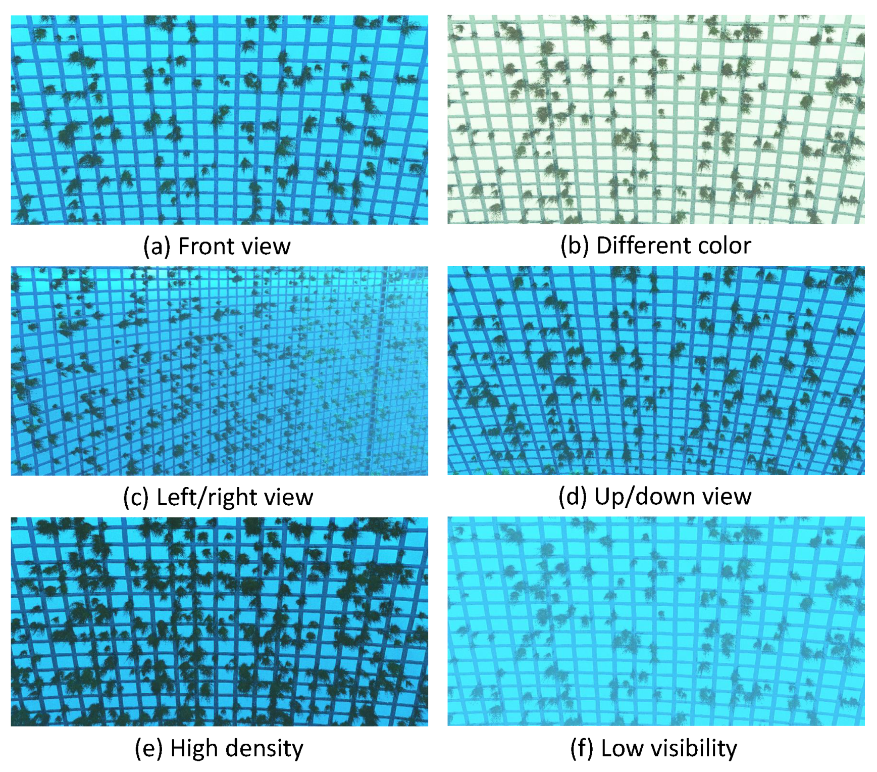
3.4.1. Variations in Image Capture Angles

Due to the uncertainty of the underwater environment, it is difficult to guarantee that every captured image is in front view. This section simulates this situation to test the effect of the algorithm on images collected from different angles as shown in Figure 9c,d.

The first four rows in

Table 2. Quantitative evaluation results on the VFN dataset.

	Seg. Eval.			Struc. Eval.		Bloc. Eval.
	Precision↑	Recall↑	F1-Score↑	mIoU↑	stdIoU↓	PCC↑	mError↓
Front	0.9892	0.9439	0.9660	0.8776	0.0539	0.9715	0.0616
Left/Right	0.9414	0.9269	0.9328	0.8313	0.0770	0.9253	0.0690
Up/Down	0.9808	0.9327	0.9561	0.8690	0.0630	0.9430	0.1652
Mean of angles	0.9705	0.9345	0.9516	0.8593	0.0646	0.9466	0.0986
Color	0.9853	0.9544	0.9695	0.8932	0.0582	0.9778	0.0466
Density	0.9618	0.9548	0.9583	0.8630	0.0899	0.9757	0.0546
Visibility	0.9848	0.9553	0.9698	0.8958	0.0530	0.9765	0.0574
Mean of all	0.9739	0.9447	0.9617	0.8717	0.658	0.9616	0.0757

show the performance on each kinds of angles and the mean of them. The performance of the most distorted image, i.e., Left/Right view as shown in Figure 9, is slightly decreased compared with Front and Up/Down views, but it is still competitive. Overall, the mean F1-score, which reaches 0.9516, implies the Underwater Image De-hazing (Section 2.1.2) and Marine Growth Segmentation (Section 2.2) modular achieved convincing performance. For the net-opening location evaluation, mIoU and stdIoU are 0.8593 and 0.0646, respectively, which means that the net-opening structure analysis module can locate the hole position. Moreover, PCC and mean Error indicate the estimation and GT have high correlation and distribution, but low error.

3.4.2. Variations in Underwater Situations

Different water areas have different ecological environments, which also lead to different water quality. In order to test the robustness and universality of the algorithm in practical applications, this section discusses the effect of the algorithm in different colors, visibility, and density of marine growth.

As shown in Table 2, the PCC values in the three scenarios are all greater than 0.97, which means that the NHSE can accurately estimate the congestion in the selected area. At the same time, the average error value is less than 0.057, indicating that the estimation of the degree of blockage in each cell area is reliable.

3.4.3. Conclusions

The experimental results, as illustrated in the last row of Table 2, on the VFN dataset show that the proposed NHSE algorithm can deal with complex underwater conditions and give reliable estimation results, and has high practicability.

3.5. Qualitative Evaluation

To comprehensively demonstrate the performance of the proposed NHSE, we show several estimation and the corresponding intermediate results including segmentation and structure results in Figure 12. Estimation results in Figure 12f indicate that NHSE can predict the blocked percentage accurately, which is consistent with RoI in Figure 12a. For example, in the first row of Figure 12, the net holes in the left corner of RoI are severely blocked, which is correctly estimated by NHSE in Figure 12f.

Again, for virtual scenes, as shown in Figure 13, samples in different virtual scenes are selected. The segmentation results and structure estimation results are consistent with GT in most cases, and accurate blocked percentage estimation results are obtained. The sample in row two, which is collected from the boundary part of the raw Right/Left view image, has some distortion in color and more noise, which leads to unsatisfactory structure estimation result, while the blocked percentage basically consistent results with GT. It further illustrates the stability of the algorithm in extreme cases.

4. Discussion and Conclusions

An underwater fishing Net Health State Estimation (NHSE) method is proposed in this work, which consists of pre-processing, marine growth segmentation, and net health estimation modules. NHSE can be utilized for the underwater images taken by ROV at any situations, and gives an estimated blocked percentage for each cell. In order to verify the scalability and robustness of the algorithm, we also built a virtual farm and collected virtual fishing net data under different conditions including angle, color, density of marine growth, and visibility. Seven evaluation metrics are introduced to demonstrate the effectiveness and practicality of NHSE.

References

- Chen, J.H.; Sung, W.T.; Lin, G.Y. Automated monitoring system for the fish farm aquaculture environment. In Proceedings of the 2015 IEEE International Conference on Systems, Man, and Cybernetics, Hong Kong, China, 9–12 October 2015; pp. 1161–1166. [Google Scholar]
- Cordova-Rozas, M.; Aucapuri-Lecarnaque, J.; Shiguihara-Juárez, P. A Cloud Monitoring System for Aquaculture using IoT. In Proceedings of the 2019 IEEE Sciences and Humanities International Research Conference (SHIRCON), Lima, Peru, 12–15 November 2019; pp. 1–4. [Google Scholar]
- Wahjuni, S.; Maarik, A.; Budiardi, T. The fuzzy inference system for intelligent water quality monitoring system to optimize eel fish farming. In Proceedings of the 2016 International Symposium on Electronics and Smart Devices (ISESD), Bandung, Indonesia, 29–30 November 2016; pp. 163–167. [Google Scholar]
- Hairol, K.N.; Adnan, R.; Samad, A.M.; Ruslan, F.A. Aquaculture Monitoring System using Arduino Mega for Automated Fish Pond System Application. In Proceedings of the 2018 IEEE Conference on Systems, Process and Control (ICSPC), Melaka, Malaysia, 14–15 December 2018; pp. 218–223. [Google Scholar]
- Luo, S.; Li, X.; Wang, D.; Sun, C.; Li, J.; Tang, G. Intelligent tuna recognition for fisheries monitoring. In Proceedings of the 2015 12th International Computer Conference on Wavelet Active Media Technology and Information Processing (ICCWAMTIP), Chengdu, China, 18–20 December 2015; pp. 158–162. [Google Scholar]
- Huang, T.W.; Hwang, J.N.; Romain, S.; Wallace, F. Fish tracking and segmentation from stereo videos on the wild sea surface for electronic monitoring of rail fishing. IEEE Trans. Circuits Syst. Video Technol. 2018, 29, 3146–3158. [Google Scholar] [CrossRef]
- Li, C.Y.; Guo, J.C.; Cong, R.M.; Pang, Y.W.; Wang, B. Underwater image enhancement by dehazing with minimum information loss and histogram distribution prior. IEEE Trans. Image Process. 2016, 25, 5664–5677. [Google Scholar] [CrossRef] [PubMed]
- Christensen, J.H.; Mogensen, L.V.; Galeazzi, R.; Andersen, J.C. Detection, Localization and Classification of Fish and Fish Species in Poor Conditions using Convolutional Neural Networks. In Proceedings of the 2018 IEEE/OES Autonomous Underwater Vehicle Workshop (AUV), Porto, Portugal, 6–9 November 2018; pp. 1–6. [Google Scholar]
- O’Byrne, M.; Ghosh, B.; Schoefs, F.; Pakrashi, V. Applications of Virtual Data in Subsea Inspections. J. Mar. Sci. Eng. 2020, 8, 328. [Google Scholar] [CrossRef]
- O’Byrne, M.; Pakrashi, V.; Schoefs, F.; Ghosh, B. Semantic segmentation of underwater imagery using deep networks trained on synthetic imagery. J. Mar. Sci. Eng. 2018, 6, 93. [Google Scholar] [CrossRef]
- He, K.; Sun, J.; Tang, X. Single image haze removal using dark channel prior. IEEE Trans. Pattern Anal. Mach. Intell. 2010, 33, 2341–2353. [Google Scholar] [PubMed]
- O’Byrne, M.; Schoefs, F.; Pakrashi, V.; Ghosh, B. An underwater lighting and turbidity image repository for analysing the performance of image-based non-destructive techniques. Struct. Infrastruct. Eng. 2018, 14, 104–123. [Google Scholar] [CrossRef]
- Narasimhan, S.G.; Nayar, S.K. Vision and the atmosphere. Int. J. Comput. Vis. 2002, 48, 233–254. [Google Scholar] [CrossRef]
- Fattal, R. Single image dehazing. ACM Trans. Graph. 2008, 27, 1–9. [Google Scholar] [CrossRef]
- Arthur, D.; Vassilvitskii, S. k-means++: The Advantages of Careful Seeding. In Proceedings of the Eighteenth Annual ACM-SIAM Symposium on Discrete Algorithms. Society for Industrial and Applied Mathematics, Philadelphia, PA, USA, 7–9 January 2007; pp. 1027–1035. [Google Scholar]
- Tan, R.T. Visibility in bad weather from a single image. In Proceedings of the 2008 IEEE Conference on Computer Vision and Pattern Recognition, Anchorage, AK, USA, 23–28 June 2008; pp. 1–8. [Google Scholar]
- Pakrashi, V.; Schoefs, F.; Memet, J.B.; O’Connor, A. ROC dependent event isolation method for image processing based assessment of corroded harbour structures. Struct. Infrastruct. Eng. 2010, 6, 365–378. [Google Scholar] [CrossRef]