A-Priori Calibration of a Structured Light Underwater 3D Sensor

Abstract

In this study, we introduce a new calibration method for underwater optical stereo scanners. It uses air calibration, additional underwater parameters, and extended camera modeling. The new methodology can be applied to both passive photogrammetric and structured light three-dimensional (3D) scanning systems. The novel camera model uses a variable principal distance depending on the radial distance to the principal point instead of two-dimensional distortion functions. This allows for an initial improvement of 3D reconstruction quality. In a second step, certain underwater-specific parameters—such as refraction indices, glass thickness, and view-port distances—are determined. Finally, a correction function for the entire measurement volume can be obtained from a few underwater measurements. Its application further improves the measurement accuracy. Measurement examples show the performance of the new calibration method in comparison to current underwater calibration strategies. A discussion of the possibilities and limits of the new calibration method and an outlook for future work complete this work.

1. Introduction

Capturing objects under water and generating three-dimensional (3D) geometric models has become increasingly important in various fields of application, such as inspection tasks of industrial structures of energy production [1,2], biologic objects [3,4,5,6], shipwrecks [7,8], or archaeological sites and objects [8,9,10,11,12]. Depending on the specific application, several techniques have been established for underwater 3D object acquisition, i.e., underwater photogrammetry [3,5,7,12,13,14,15], laser scanning techniques [1,2,16,17,18,19], ultrasound sensors [20], and time-of-flight methodology [21]. Each of these techniques have advantages and disadvantages.

Photogrammetric measurements typically provide high spatial object point resolution and high measurement accuracy. The field of view of the cameras may be several square meters. However, preparation of the scene by placing landmarks onto or nearby the objects might require high effort. Additionally, photogrammetric underwater measurements typically require non-moving scenes and scanner fixation, e.g., on a tripod.

Laser scanning systems for underwater 3D acquisition are commercially available [19]. These systems can measure distances up to 40 m. Furthermore, they are suitable for application in polluted water. However, due to the line-scanning measurement principle, spatial and temporal resolution of the captured object points is limited.

Scanners using structured light projection techniques have been introduced for underwater 3D measurements in the past few years [21,22,23,24,25,26]. This technique provides some advantages over passive photogrammetry and laser scanning. More 3D points with higher spatial density can be captured, enabling a more detailed 3D reconstruction of the observed object. As no scene preparation is required, this measurement principle is versatile and allows for relative movements up to a certain velocity. Measurement data are obtained immediately and can be subsequently processed. The main disadvantage that have prevented wide commercial applicability is the necessity of a high-power lighting system. Consequently, recent systems have a small field of view and a short measurement distance.

Calibration of the 3D scanning system is essential for the accuracy and responsible for the systematic errors of the measurements. An excellent and extensive overview of camera calibration techniques for accurate underwater measurements is given by Shortis [27].

One strategy to obtain underwater calibration parameters is to analogously perform the calibration on classical air calibration, for instance using a chessboard [28] or other calibration targets [27] in a water basin under comparable conditions (e.g., temperature, salinity, pressure) to the place of measurement. The pinhole camera model can be used and the loss of a single viewpoint (projection center) is neglected. Refraction effects lead to distortions that can be described in the same manner as in air calibration. However, remaining deviations and errors will be larger than in air case due to ray refraction, especially when the measurement depth is extensive.

Considering the refraction at the media boundary, the camera model must be modified. Here, the works of Telem and Filin [15], as well as Sedlacek and Koch [14,29] provide solutions under consideration of all underwater environment conditions.

In previous studies [26,30], we developed a calibration method using air calibration according to the classical pinhole model with distortion correction and a subsequent determination of underwater parameters using at least four underwater measurements. In this work, we further developed this model by replacing the radial distortion function by a variable principal distance and a-priori estimation of underwater parameters. Finally, a refinement of the calibration was achieved by determining a 3D correction function over the measurement volume.

The goal of this work was to develop a methodology for an easy-to-handle pre-calibration of underwater optical stereo 3D scanners based on photogrammetric principles using conventional air calibration and an adapted camera modeling. In our experiments, we showed that the new methodology can be successfully applied to such scanners. However, in order to achieve highest measurement accuracy, additional calibration effort is necessary.

We used data of a handheld 3D underwater stereo scanner with structured light projection for a measurement volume of 250 mm × 200 mm × 100 mm.

2. Materials and Methods

Recent photogrammetric underwater applications of 3D scanning required high effort with regard to both preparation of the measurements and calibration of the scanner. In order to achieve high measurement accuracy, refraction of the vision rays at the boundary between the different media (air to glass and glass to water) must be taken into account. Recently, a number of different models were developed [14,15,31].

The goal of this work was to generate a set of calibration parameters for achieving the best measurement accuracy without any underwater measurements or, optionally, with minimal effort of underwater measurements. The strategy includes a novel geometric modeling of radial lens distortion and estimation of several parameters.

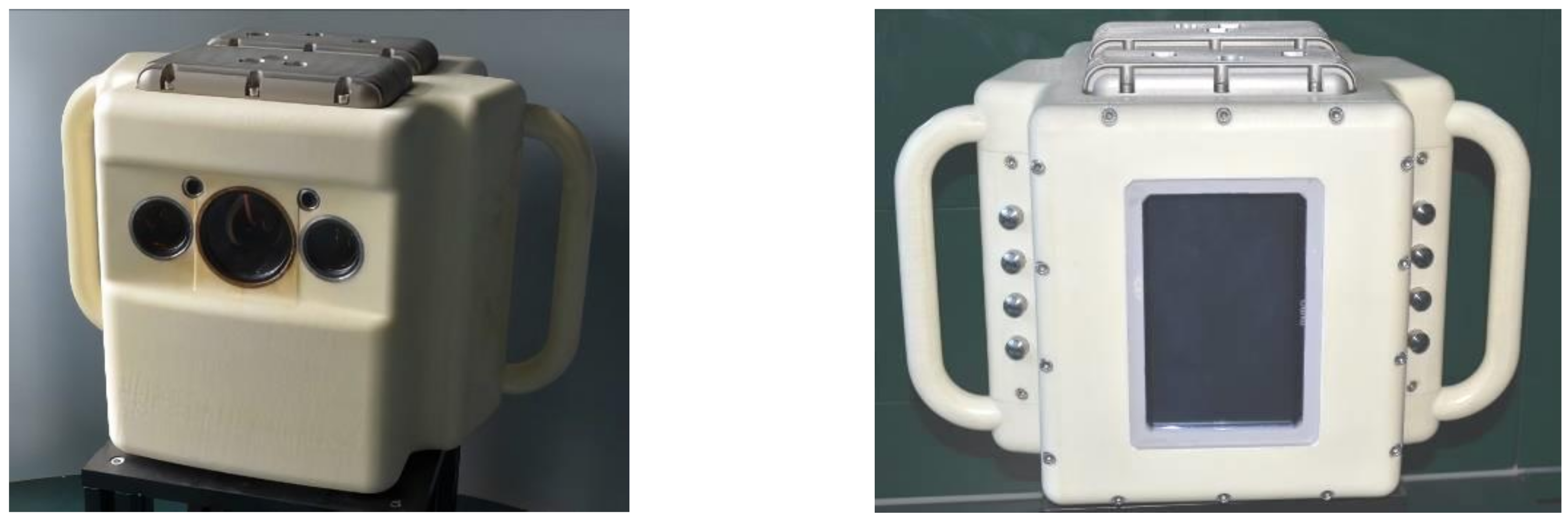
The new methodology was developed for a-priori calibration of underwater 3D stereo scanners. Our scanner is a hand-held underwater 3D scanner that covers a measurement volume of approximately 250 mm × 200 mm × 100 mm [26]. It has plane viewports adjusted in perpendicular direction to the principal rays of the cameras. This property is used as a constraint to the extended model described in the following section.

2.1. Extended Pinhole Camera Model

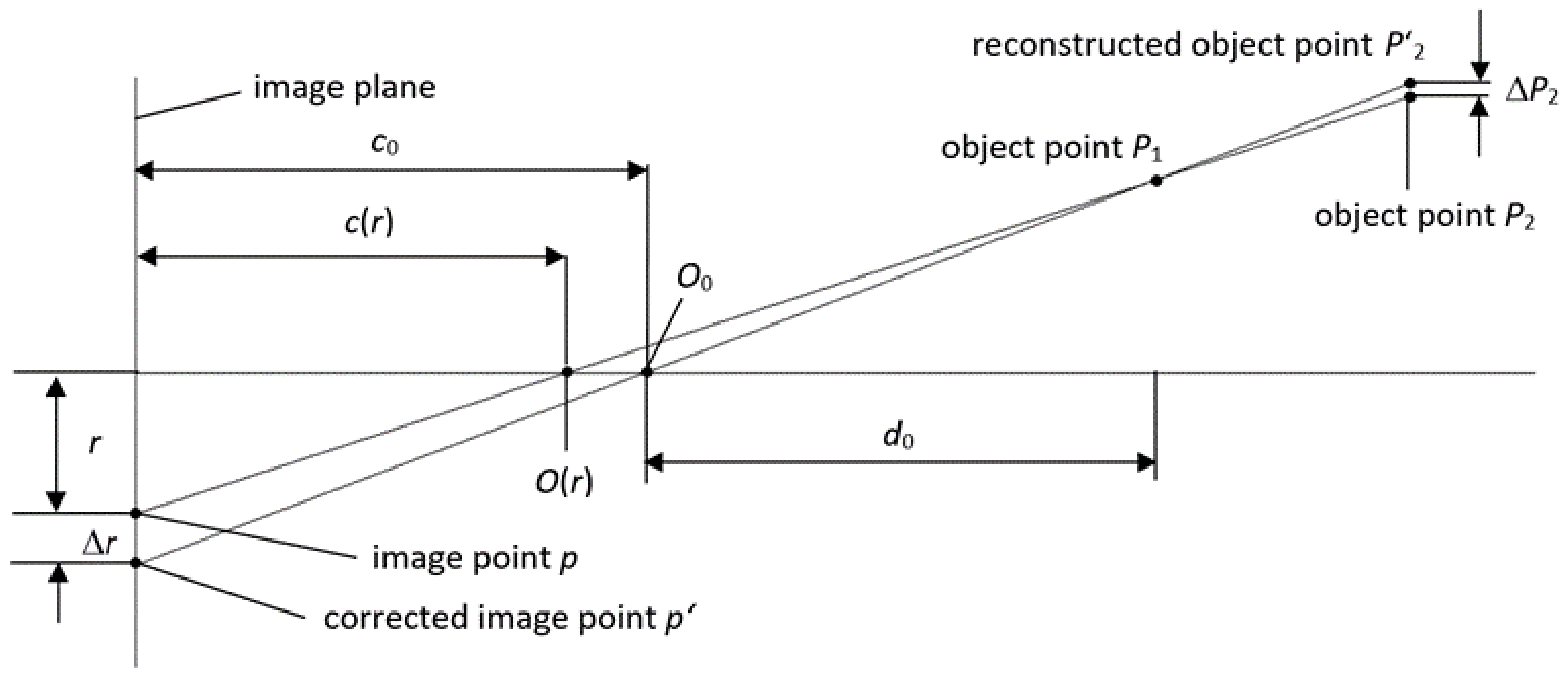
Typically, for stereo-photogrammetric 3D reconstruction, the common pinhole model (PM) is extended by so-called distortion functions. These distortion functions are mainly lens-dependent but also take inhomogeneities of the image sensor and adjustment deviations into account. Generally, distortion functions are described by several functional parameters or matrices of correction vectors. Considering the pinhole model, distortion correction leads to deviation of the vision rays in the projection center. Physically, however, vision rays do not pass through the projection center but close nearby. Pinhole-style modeling implies that correct 3D reproduction is achieved only for one certain plane in the measurement volume. At other distances, systematic errors appear in the reconstruction of the 3D points. These errors are typically neglected because their amount is below the noise level. However, at short measurement distances, these errors may become significant. A typical limit for significance is a magnification factor larger than 1/30, i.e., a measurement distance below 30 times the focal length of the lens for high-accuracy measurements.

For extended modeling, we assumed that vision rays passing close to the projection center O₀ intersected the optical axis in the point O(r). The higher the radial distance r of the point p to the principal point p₀, the farther the intersection point O(r) to O₀, i.e., in direction to the sensor image plane.

Common modeling uses the PM and a 2D correction function for distortion effects and assumes optimal parameter determination via calibration, thus leading to ideal results for just one object plane in the measurement volume. Reconstructed points outside this plane have certain systematic errors. The size of these errors correlates with the distortion function and can be approximated from the parameters of the distortion function. Assuming a typical measurement volume, the systematic errors are quite small and significantly smaller than the typically occurring random measurement errors. Consequently, these systematic errors can be neglected. In case of underwater measurements, however, they may increase due to refraction effects. Hence, the errors must be considered and compensated, or a new model avoiding these errors must be used. This new model will be introduced in the following section. It should be called “extended pinhole model with variable principal distance”.

2.2. Alternative Modeling of Radial Distortion

The common radial distortion function is typically described by a polynomial in the sensor image plane is replaced by a variable principal distance. All other non-radial parts of distortion are neglected, because the amount of the radial parts typically is about 95% of the total distortion. The modeling by variable principal distance is close to the physical truth at image generation and leads to the effect that no distance-dependent errors occur at distortion correction. This is illustrated in Figure 1. Only points at distance d₀ are properly corrected by Δr (e.g., point P₁ in Figure 1), whereas other points such as P₂ are erroneously corrected with reconstruction error ΔP₂. Using variable principal distance, all points are correctly reconstructed.

Instead of a polynomial over r in the image plane, a variable principal distance c(r) and an appropriately shifted projection center O(r) is used. Determination of c(r) may be realized in different ways and calculated according to Equation (6) (see Section 2.3 (calibration)). In case of calculating 3D points by triangulation using a stereo camera setup, every image point has its own variable principal distance c(r) and its own projection center O(r).

A precondition for calculating 3D coordinates is the determination of proper point correspondences. They cannot be directly obtained from rectified images [32], as this would require the common pinhole camera model. However, if function c(r) is known, appropriate correction values can be calculated. Thus, correspondence finding can be realized iteratively in rectified images and an estimated pinhole model can be used as first approximation.

2.2.1. Transition to the Underwater Case

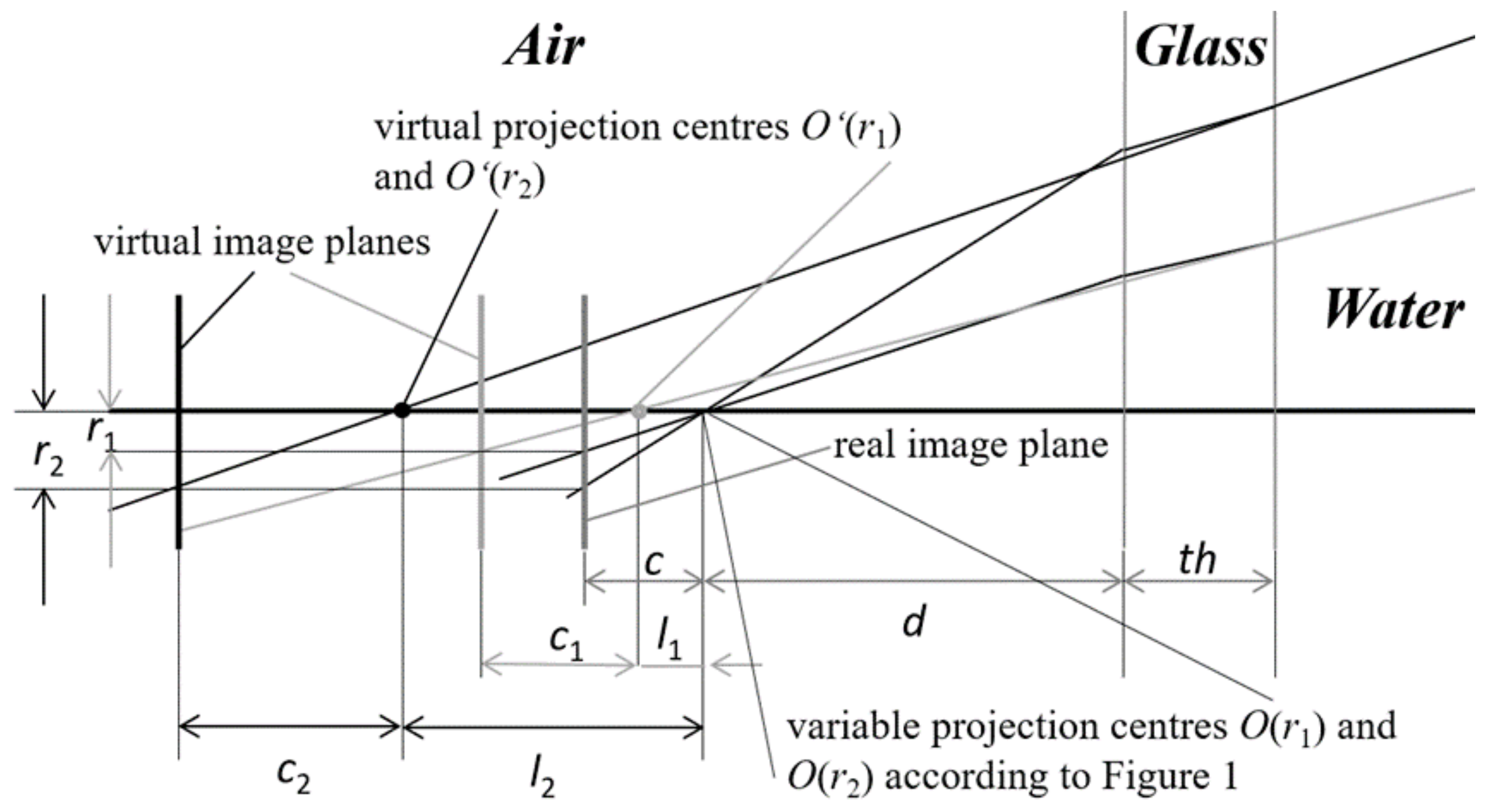
As previously shown by the authors [26], vision rays are refracted at the boundary between air and glass in the housing, and between glass and water outside the housing according to certain parameters, like refraction indices, glass thickness, distance between camera, and vision glass. In order to correctly reconstruct the scene, changed ray courses must be determined and inserted into the reconstruction calculation. Accordingly, considering a variable principal distance c(r), radially dependent virtual principal distance c’(r) for the underwater case leads to:

$$c’\left(r\right)=\frac{r}{\tan \left(\arcsin \left(\frac{\sin \left(\arctan \left(r/c(r)\right)\right)}{n_w}\right)\right)}$$

(1)

For the translation of the projection center this means:

$$l\left(r\right)=l_w\left(r\right)+l_g\left(r\right)$$

(2)

with $l_w\left(r\right)=d\left(1-\frac{r}{c\cdot \tan \left(\arcsin \left(\frac{\sin \left(\arctan \left(r/c\left(r\right)\right)\right)}{n_w}\right)\right)}\right)$, $l_g\left(r\right)=th\left(1-\frac{c}{r}\cdot \tan \left(\arcsin \left(\frac{\sin \left(\arctan \left(r/c\left(r\right)\right)\right)}{n_g}\right)\right)\right)$, where th is the thickness of the glass, n_w refraction index of water, and n_g refraction index of glass. The refraction index of air is set to n_a = 1.0 and is omitted in the equations. For the new projection centers O’(r) it holds:

$$O’\left(r\right)=O\left(r\right)-l\left(r\right)\cdot R\cdot e$$

(3)

where O(r) is the initially determined projection center of the camera outside housing according to the pinhole model, e is the unit vector, and R is the rotation matrix describing the deviation of the principal ray of the camera according to the pinhole model calibration. Figure 2 shows the vision ray course for two image points with different distances to the principal point.

Application of Formulas (1)–(3) can be realized by using extended software modules according to the common methods (see Luhmann et al. [33]). Non-radial distortion effects can be compensated by application of additional functions. Finally, remaining errors may be compensated by a 3D correction function in the measurement volume [34]. It is expected that significant errors may remain, because some assumptions are very simplifying (e.g., the assumed orientations of the principal rays in relation to the glass surfaces of the housing ports). Determination of corresponding correction functions can be realized in a final calibration step (see Section 2.3 calibration).

2.2.2. Simplified Pinhole Model for Underwater Application

When using existing photogrammetric software for the underwater 3D reconstruction, the method described in the following should be applied.

As described before, every image point p_i = (x_i,y_i) has its own individual principal distance and own projection center, depending on the radial distance to the principal point p₀ = (x₀,y₀). Parameters are refraction indices, glass thickness, distance between camera and glass, and variable principal distances.

Both experiments and simulations using parameters close to real conditions have shown that the variance of c’(r) and O’(r) is relatively small. This is due to the fact that the variable principal distance in air is smaller for big radial distances, but larger in water. Hence, both effects partly compensate, which leads to the assumption that if using a fixed principal distance and a fixed projection center (if as using the classical pinhole model) only causes a small error in the 3D point calculation. For known parameters, the error can be estimated a-priori. Furthermore, it can be described and compensated for a plane at a certain distance in water by a classical radial distortion function or distortion matrix. Additionally, remaining errors due to deviation of the points from the reference plane can be appropriately predicted by calculation.

Fixed principal distance c’ (and fixed projection center O’ analogously) can be chosen as average values over all image points:

$$c’=\frac{1}{n}{\displaystyle \sum _{i=1}^{n}c’\left(r_i\right)};r_i=\sqrt{\left(x_i-x_0\right)+\left(y_i-y_0\right)}$$

(4)

Distortion function is valid for reference plane E₀, being in distance d₀ to the projection center O’. Accordingly, E₀ should be adjusted parallel to the image plane. If the camera sensor planes are not parallel, two different reference planes E₁ and E₂ may be chosen, and the common reference plane E₀ is obtained by averaging E₁ and E₂. Distortion will be calculated by:

$$\Delta r=r\cdot \left(\frac{c_0\cdot \left(l\left(r\right)+d_0\right)}{c’\left(r\right)\cdot \left(len+d_0\right)}-1\right)$$

(5)

Here, len is a fix value for shifting the projection center which can be chosen as average value over all l(r).

This model can be checked or replaced by a classical model by a pinhole calibration directly performed under water. It should be noted, however, that distance-dependent distortion effects are considerably larger than at air application of the scanner. However, the expected errors can be derived using Formulas (1)–(3).

2.3. Calibration

Calibration is performed in three steps and completely in air. Optionally, a fourth calibration step, which requires underwater measurements, can be added. The first step is identical to classical air calibration where intrinsic (principal distance, principal point, distortion) and extrinsic (relative orientation between the stereo cameras) parameters are determined in the world co-ordinate system (WCS).

Depending on the technical realization of the sensor hardware, air calibration is performed without or inside underwater housing. Accordingly, glass thickness and glass material (refraction index) must be considered. From the two-dimensional radial distortion function, the variable principal distance c(r) can be estimated with c₀ as principal distance of the air calibration and assuming a main reference distance d₀ at air calibration:

$$c\left(r\right)=\frac{r\cdot \left(d_0+c_0\right)}{r+d_0/c_0\left(r+\mathrm{\Delta }r\right)}$$

(6)

Naturally, this estimation is erroneous, because the determination of the radial distortion within intrinsic calibration is erroneous, too. However, due to the new modeling concept, these errors are reduced. Alternatively, c(r) can be determined separately by goniometric measurements. However, the risk of high random errors is high. The corresponding error cannot be determined because there does not exist any reference method. As we will see later in Section 3, extended modeling with variable principal distance actually leads to decreased systematic 3D measurement errors at air calibration.

The second step of calibration comprises determination of refraction indices, glass thickness, and distance between the camera and housing ports. The glass thickness can be measured and the refraction indices are known for the materials used. The refraction index of water depends both on temperature and salinity. The distances d₁ and d₂ between the two cameras to the housing ports may be estimated using the hardware design and possibly refined after performance of underwater measurements [26]. However, first experiments and simulations have shown a very weak dependence of the resulting 3D reconstruction error on the values of d₁ and d₂. Actually, an uncertainty of d₁ and d₂ of some millimeters lead to errors of few micrometers in the 3D measurement and can be typically ignored.

In the third step of underwater calibration the parameters for the 3D calculation according to Equations (1)–(3) are determined.

The quality of this calibration can be evaluated by four (or more) underwater measurements of planes and ball-bars in a certain arrangement. These measurements characterize the quality of the calibration by determination of certain characteristic quantities (e.g., length measurement deviation, flatness deviation [35]). Alternatively, they may serve for determination of a 3D correction function, which can be understood as the fourth step of the calibration process. This fourth step should be performed in accordance to the estimated remaining errors and the requirements to the measurement accuracy, if required.

The minimal number of evaluation measurements in order to estimate low-frequency systematic errors is four: two plane measurements M₁ and M₂ at the front and the back of the measurement volume (MV), and two (M₃ and M₄) ball-bed measurements in the same regions in the MV. These measurements can be used to estimate the distribution of the systematic error in the MV [34] and a correction function can be defined. This function may be a polynomial in R³ or a field of 3D correction vectors at certain sampling points. It corrects the 3D measurement points depending on the distance and the radial displacement to the main axis of the sensor (which can be constructed as average of both optical axis of the cameras).

2.4. Material

In order to evaluate the proposed new methodology for a-priori calibration of optical underwater 3D scanners recordings of a hand-held underwater 3D scanner were used and compared to the results obtained from measurements using the calibration method proposed in [26]. Figure 3 shows the scanning device. Calibration was initially performed without housing using the commercially available software BINGO [36]. Afterwards, measurements were performed in order to evaluate the air calibration and to assess the effects of the use of the extended pinhole model with variable principal distance.

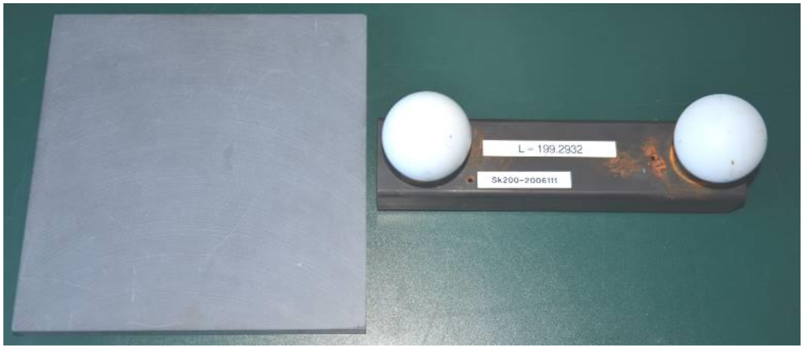
Subsequently, measurements inside housing and underwater measurements were performed. Measurement objects were a plane made of ceramics and a ball-bed with a calibrated distance between the sphere center points (see Figure 4).

3. Experiments and Results

3.1. Calibration Evaluation

Calibration of the scanner was performed using a scene without landmarks including a frustum of a pyramid and using the software BINGO. This results in a set of intrinsic and extrinsic parameters for both cameras. Distortion functions were determined by application of a number (8 of 60) of one-parametric distortion functions.

The amount of the radial symmetric distortion was 98% (left camera) and 95% (right camera), respectively. The average distance of the measured points was about 500 mm. The function c(r) was calculated at 1000 discrete values for r according to Equation (6). A third-degree polynomial was fitted to these sampling points for both cameras in order to obtain the functional description of c(r).

Subsequently, the underwater parameters were determined (

Table 1. Underwater parameters of the 3D scanner obtained from literature (refraction indices, water index is 1.0), design (viewport distance), and mechanical measurement (glass thickness).

Glass Thickness	Refraction Index Water	Refraction Index Glass	Distance to Viewport
3.0 mm	1.334	1.76	60 mm

). According to Equations (1) to (3), the functions c’(r) and l(r) were obtained in the third step of the underwater calibration.

Additionally, using the four measurements M₁ to M₄ (see Section 2.3) a 3D correction function Δv = f(x,y,z) was determined and applied according to the description in Section 2.3 as follows. Plane measurements (approximated by two planes E₁ and E₂ in the WCS) were used to correct Z coordinates described by a squared polynomial in r according to the estimated symmetry points s₁ and s₂ of the plane deformation. Correction values for points outside the planes E₁ and E₂ are obtained by linear interpolation or extrapolation. Ball-bed measurements were used to estimate the correction function in X and Y. Here, linear scaling of the points according to the radius regarding s₁ and s₂ was applied for points in E₁ and E₂ and interpolation or extrapolation was processed analogously to Z correction.

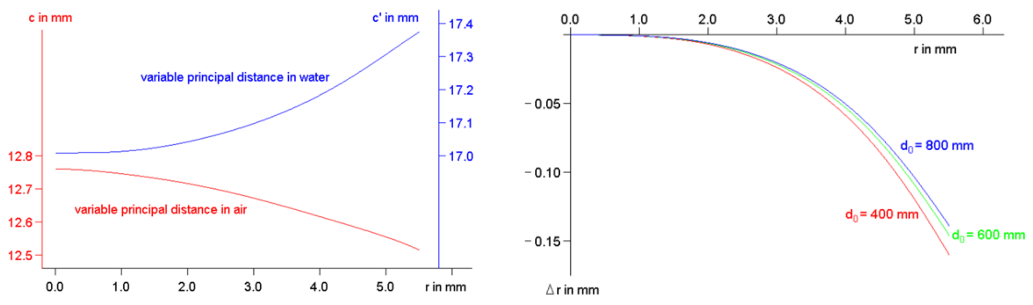
Finally, a conventional pinhole model was generated according to the description of Section 2.2.2. See Figure 5 for the function plots of c(r) in air and c’(r) in water according to Equation (1) and calculated radial distortion function Δr according to Equation (5) for three different arbitrarily chosen values for the standard distance d₀ (d₀₁ = 400 mm, d₀₂ = 600 mm, and d₀₃ = 800 mm).

3.2. Experimental Evaluation

In order to evaluate the different calibrations, several measurements of a plane and a ball-bed at different distances between 380 mm and 500 mm were performed. For evaluation, flatness deviation, and length measurement deviation were determined according to a prior description [26] and in accordance to the VDI/VDE guidelines of the “Verein Deutscher Ingenieure” [35]. First, measurements were realized without underwater housing in air. The results obtained by the common pinhole model with distortion correction was compared to the results obtained by the new modeling with variable principal length and projection center using identical measurement data.

Table 2. Comparison of air calibration cal₁ using variable principal distance (PD) and projection center to classical pinhole calibration cal₂ including distortion correction (DC) using identical measurement data.

Calibration	PD	DC	Length Error	Flatness Error
cal1	variable	no	100 µm (0.05% 1)	212 µm (0.05% 2)
cal2	fix	yes (radial and other)	145 µm (0.07% 1)	266 µm (0.07% 2)

¹ reference length was 200 mm, ² plane diagonal was between 270 mm and 400 mm.

shows the results of length and flatness deviation at air measurements.

In a second experiment, underwater measurements were performed. Characteristic quantities were determined for identical underwater measurement data using different calibrations, i.e., previous underwater calibration [26] (cal₀), new methodology with variable principal distance without (cal₁), 3D correction function (cal₂), and fix principal distance model (cal₃), according to Section 2.2.2.

Table 3. New underwater calibration method without underwater measurements (cal₁) with 3D correction polynomial (cal₂) and as approximated classical pinhole calibration (cal₃) compared to previous calibration [26] (cal₀).

Calibration	Air/Water	PD	DC	Length Error	Flatness Error
cal0	air + water	variable	yes	0.21 mm (0.11% 1)	2.5 mm (0.8%2)
cal1	air	variable	no	0.40 mm (0.20% 1)	2.0 mm (0.6%2)
cal2	air + water	variable	no	0.15 mm (0.08% 1)	1.0 mm (0.3%2)
cal3	air	fix	yes	0.87 mm (0.44% 1)	2.4 mm (0.8%2)

¹ reference length was 200 mm, ² plane diagonal was between 250 mm and 300 mm.

shows the results of length and flatness deviation in underwater measurements.

Although it is difficult to compare accuracy results of different calibration and 3D calculation methods, we compared our results with some (partly extracted) values from the literature (see

Table 4. Comparison of selected 3D accuracy results from the literature.

Author/Reference	Method	Validation	Percentage Error 1
Li et al. 1996 [37]	Photogrammetry	Length error	0.8
Telem and Filin 2010 [15]	Photogrammetry	Flatness and length error	0.1–0.4
Zhang 2011 [24]	Fringe projection	Length error	0.5
Bruno et al. 2011 [23]	Fringe projection	Flatness error	0.5
Bianco et al. 2013 [25]	Fringe projection	Flatness and length error	0.1–0.3
Buschinelli et al. 2016 [38]	Fringe projection	Length error (ball-bar)	0.4

¹ percentage error was estimated by the authors from the published error values.

). As can be seen, most error results transformed to percentage have similar magnitude. A more extensive analysis of underwater calibration methods including error quantities is presented by Shortis [27].

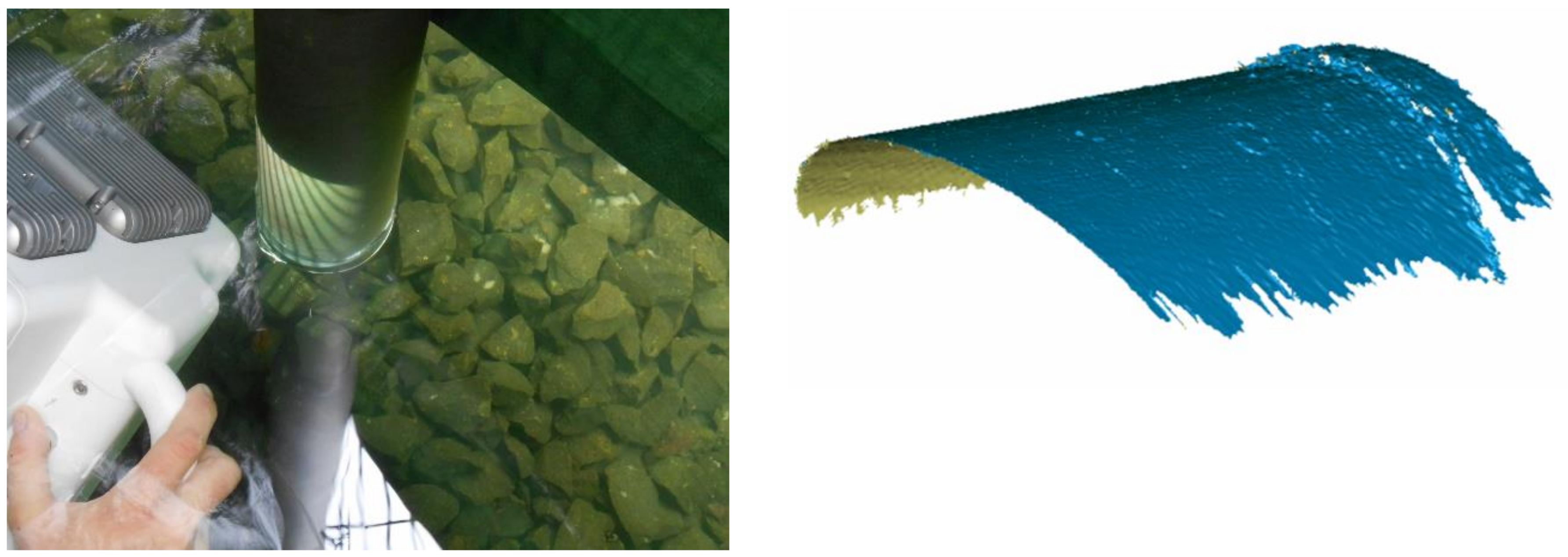
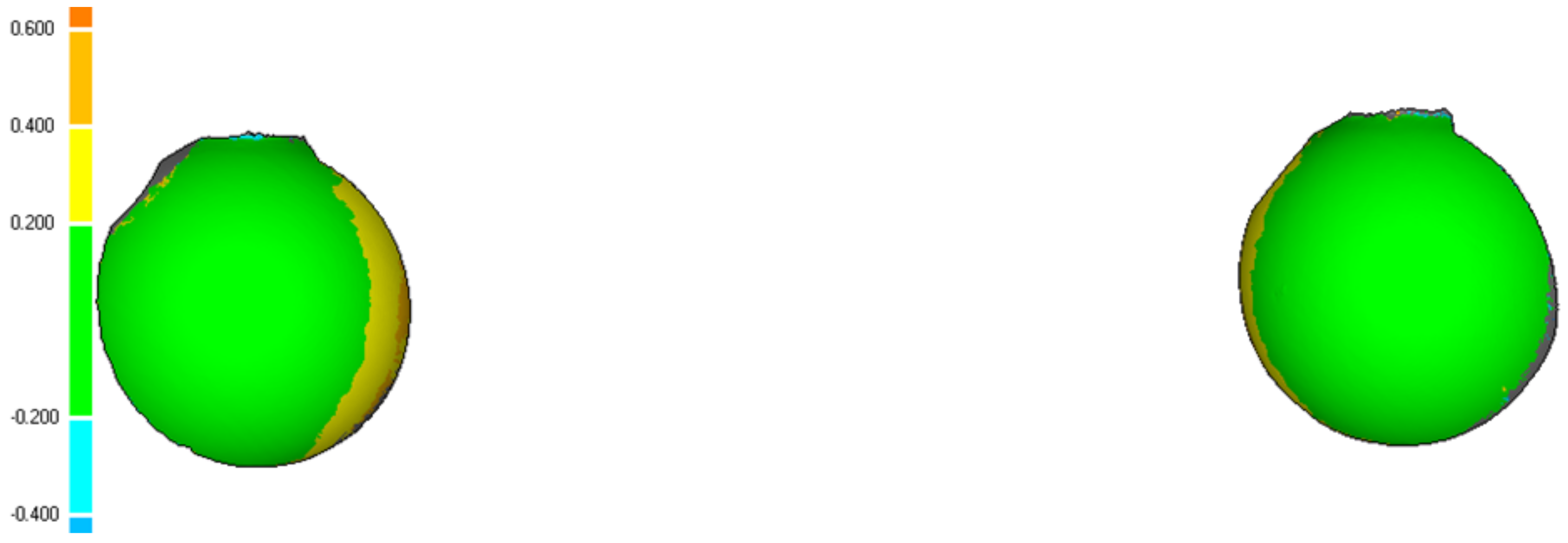
An application example of the scanner showing projected fringe pattern and 3D reconstruction result is shown in Figure 6. Figure 7 shows the difference of two ball-bed measurements in air and water, respectively. Different colors represent the deviation in the 3D comparison.

3.3. Error Consideration

The remaining errors of the new methodology may have multiple sources. As the typically used pinhole model has its deviations from reality, the new modeling with variable principal distance has deviations, too. One potential error source in this regard is the method to determine c(r). The proposed method assumes a correct distortion determination for the distance of the reference plane. However, this is only an approximation. We assume that by using a better method for finding c(r), the results can be further improved. Additionally, chromatic aberration effects may influence the determination of the distortion function or variable principal distance, respectively. Whereas at air calibration white light is typically present, blue light has greater impact to the image generation under water.

One next potential error source is the deviation from the perpendicularity between principal rays of the two cameras and glass ports of the housing. By using this as precondition, deviations may be compensated only by a 3D correction function. Deviations of the actual refraction indices from the used values seem to be negligible as well as small deviations of the parameters d₁ and d₂ (camera distances to the viewports). This was confirmed by simulations.

All deviations of the real situation from the assumed model properties lead to systematic errors of the reconstruction of the vision ray and subsequently to systematic errors of the determined 3D measurement points.

Other error sources may be inhomogeneities of media. For instance, the glass of the vision ports might contain material discontinuities.

4. Discussion

The results have shown the capability of the new methodology for calibration of a structured light optical underwater 3D stereo scanner. Additional effort with respect to classical air calibration is low. Measurement accuracy is comparable to former results and values from the literature (see [27]). Improvements regarding the 3D measurement accuracy are insignificant. Scanning object points in considerably different distances let expect to show the advantage of the new modeling concept.

By performing an additional calibration step using underwater measurements, high accuracy can be achieved using an additional correction function. The new method is advantageous for close range photogrammetric measurements, where the measurement distance is short and varying.

The presented experimental results obtained by complete air calibration (cal₁) almost achieve the results from the literature. However, for more comprehensive statements concerning measurement accuracy of the new methodology more experiments should be performed. This is one of the most important future tasks. It should be mentioned that the data used are from measurements using a very short distance to the measurement objects. In this context, local relative systematic errors are expected to be particularly high. Hence, for measurements at larger distances (e.g., 1 m), the new methodology, including the subsequent under water refinement of the calibration, provides more accurate 3D measurement results.

However, the introduced new methodology can be further improved. Certain error sources were neglected and simplifications were made. The method has not been applied to other underwater scanning devices yet.

Another shortcoming of the method is the use of a plane for determination of the additional correction function. Such a plane (material should be granite or ceramics) is easy to handle for small measurement volumes but may become cumbersome, heavy, and expensive for larger fields of view (e.g., 1 m²).

In order to overcome these remaining weaknesses of the method, future work should aim to replace the plane measurements in water by calibration bodies which can be handled more easily.

Another focus of future work should be further verification by using more measurements of underwater 3D scanners of similar type in order to confirm results.

5. Conclusions

A-priori underwater calibration of optical 3D stereo scanners is possible using the described new method. This methodology follows a new geometric modeling of the radial lens distortion, leading to a variable principal distance depending on the radial distance of the points with respect to the principal point.

Application of the new calibration method provides satisfying 3D accuracy results with low effort. It provides a good alternative to complex calibration if no high-end precision is necessary. Varying external conditions, such as water temperature and salinity, can be considered in the calibration. A post-processing correction step using a small number of underwater measurements provides an improvement of the accuracy by factor two. It is expected that further improvements are possible, which will achieve a further reduction of the remaining errors.