Experimental and Numerical Investigation on the Transport Characteristics of Particle-Fluid Mixture in Y-Shaped Elbow


Abstract
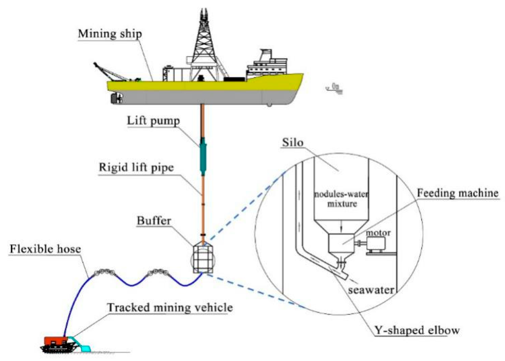
1. Introduction
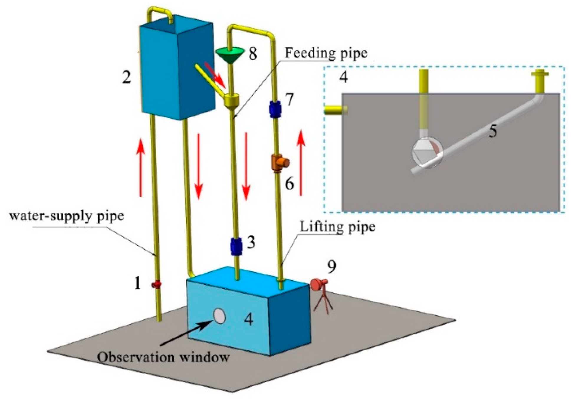
2. Experimental Platform
3. Numerical Morphology
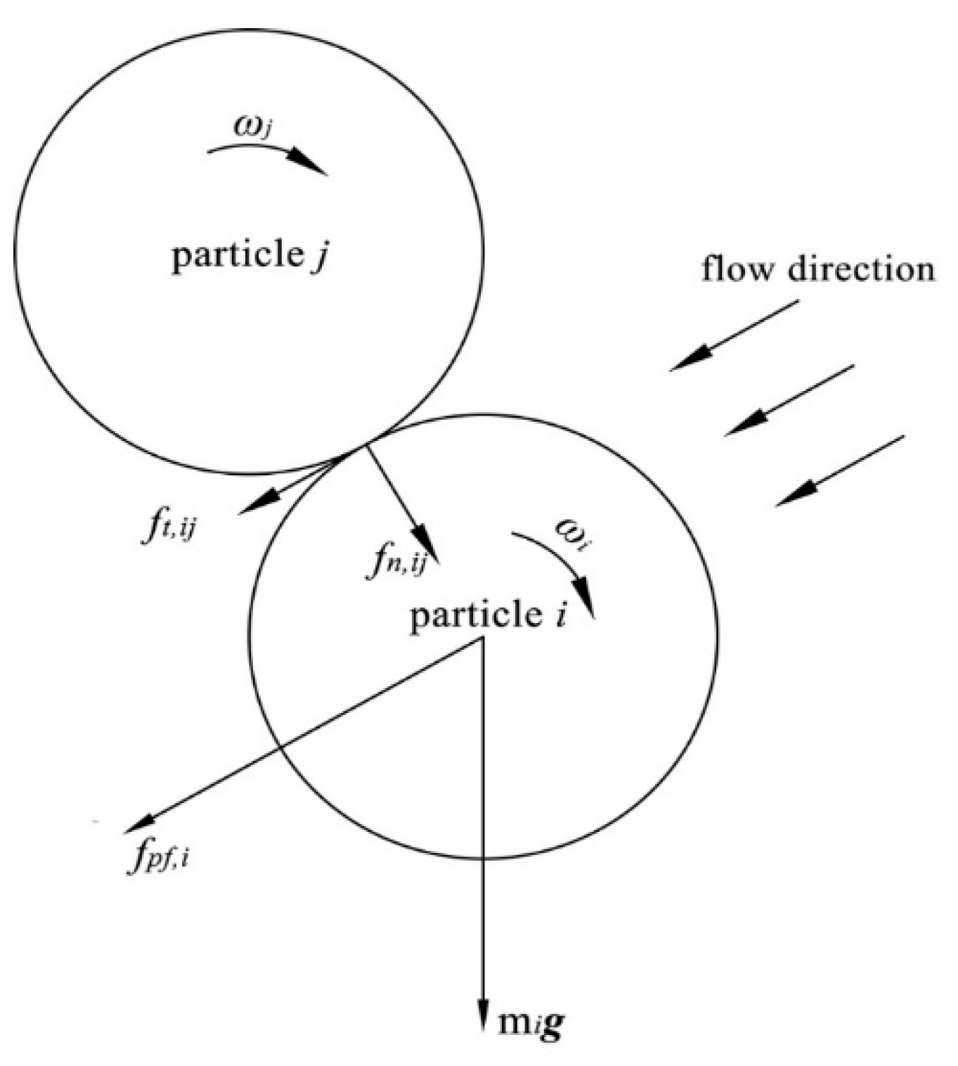
3.1. Fluid and Particle Equations
- (1)
- Continuity equation
- (2)
- Momentum equationwhere is the fluid density, ui and uj are the velocity components in Cartesian coordinates i, j, respectively, P is the static pressure of fluid, τij is the fluid viscous tensor component, g is the acceleration of gravity and Fpf is the interaction forces between continuous and discrete phases.where ffp,i stands for the interaction force between the particle i and fluid and kc is the number of particles in a CFD cell of volume ΔVc.
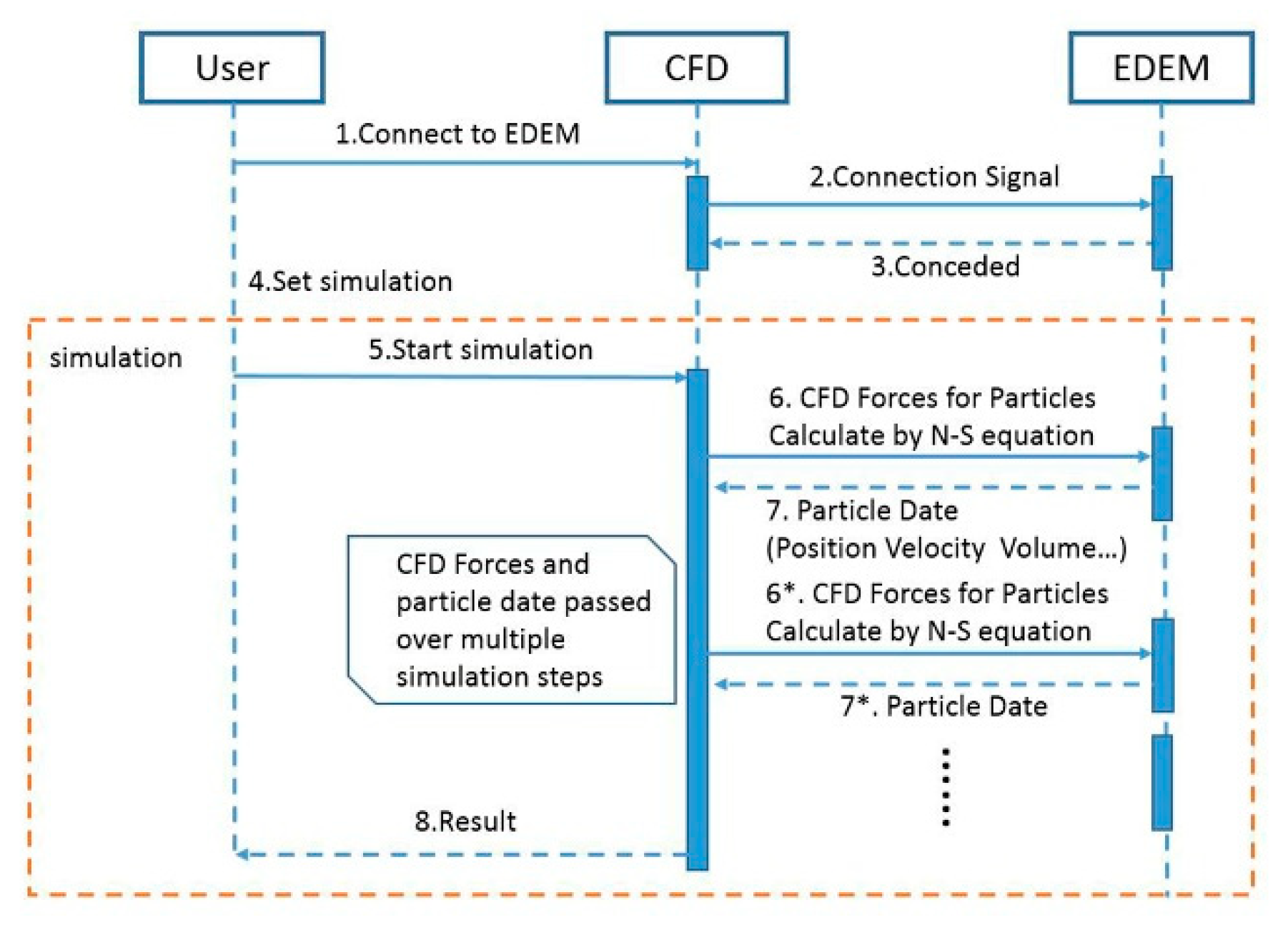
3.2. CFD-DEM Coupling Method
3.3. Y-Shaped Elbow Model and Mesh Generation
3.4. Simulation Parameters Setup
3.4.1. CFD Settings
3.4.2. EDEM Settings
4. Results and Discussion
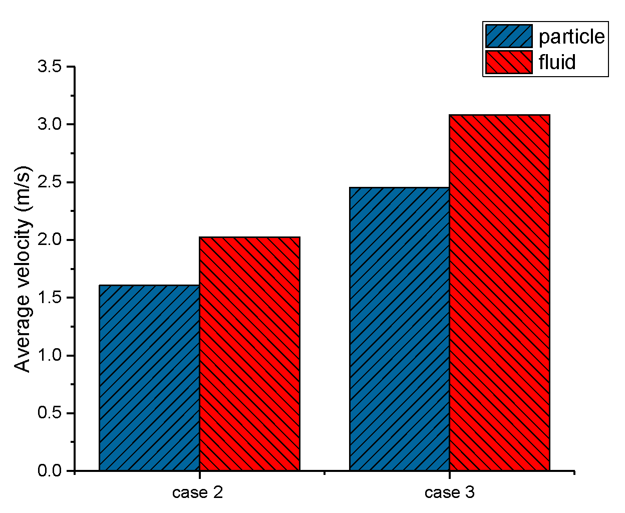
4.1. Particle Analysis
4.1.1. Particle Distribution
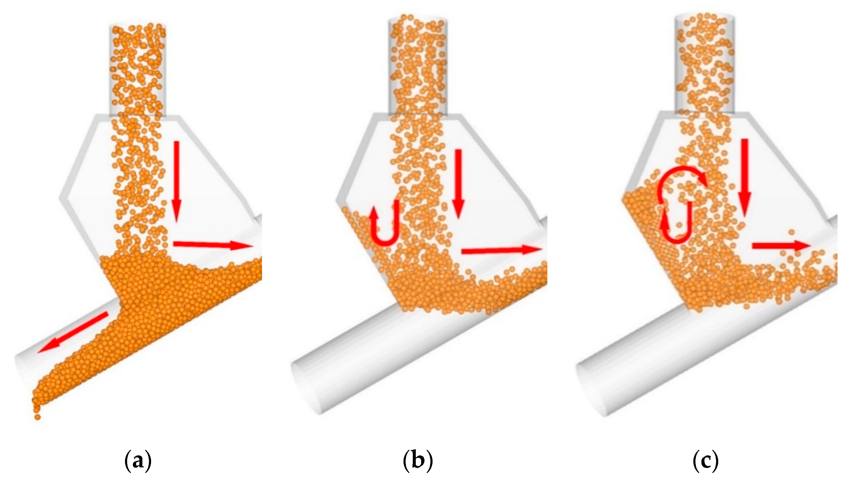
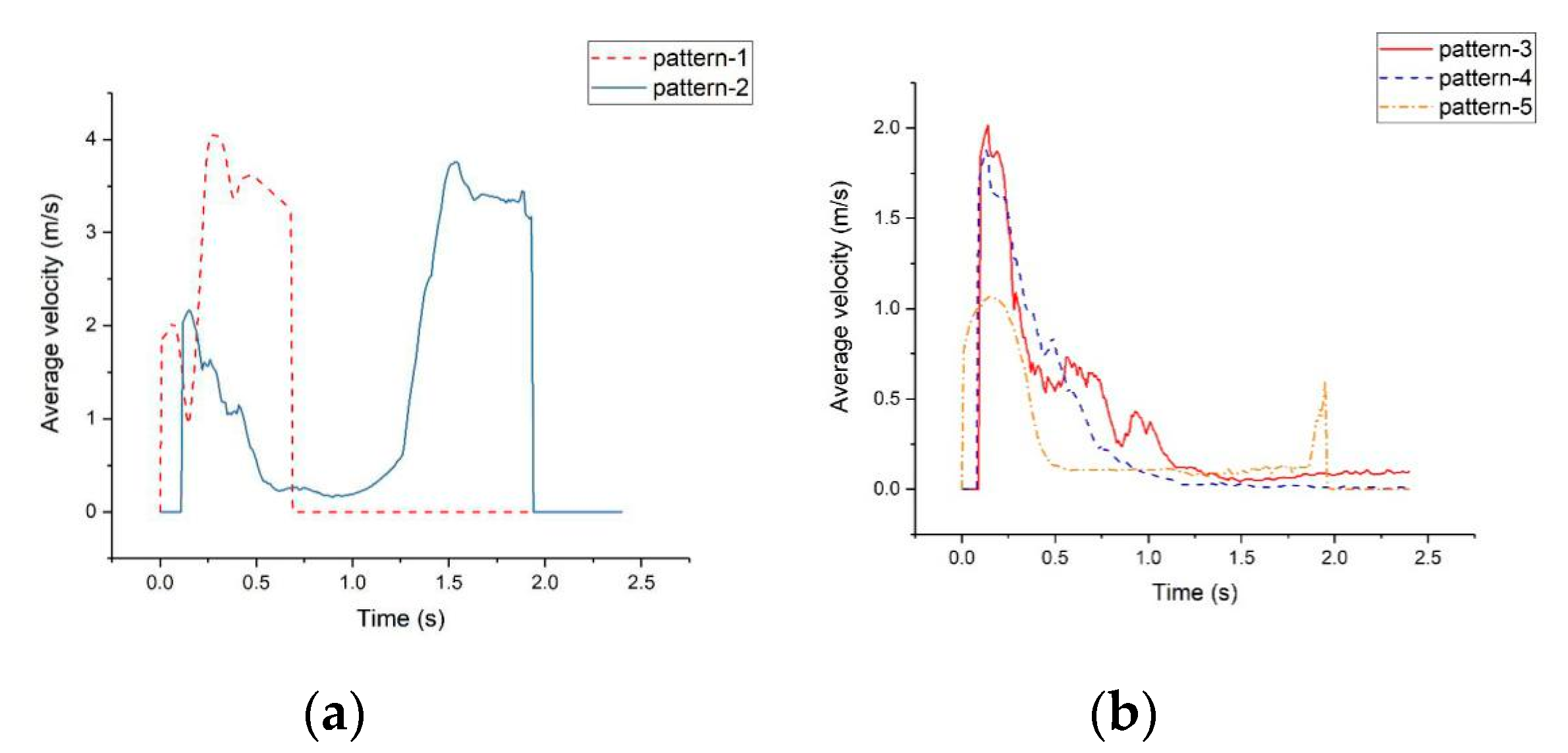
4.1.2. Particle Motions
4.2. Flow Field
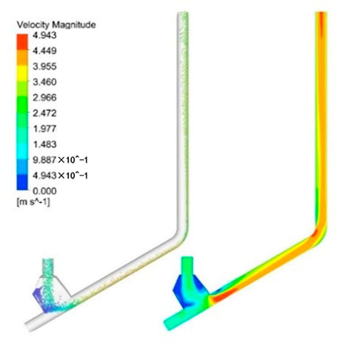
4.2.1. Contour of Velocity
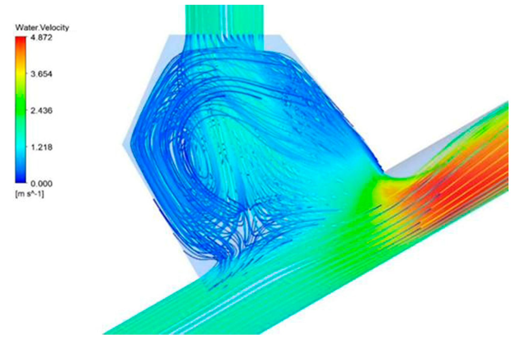
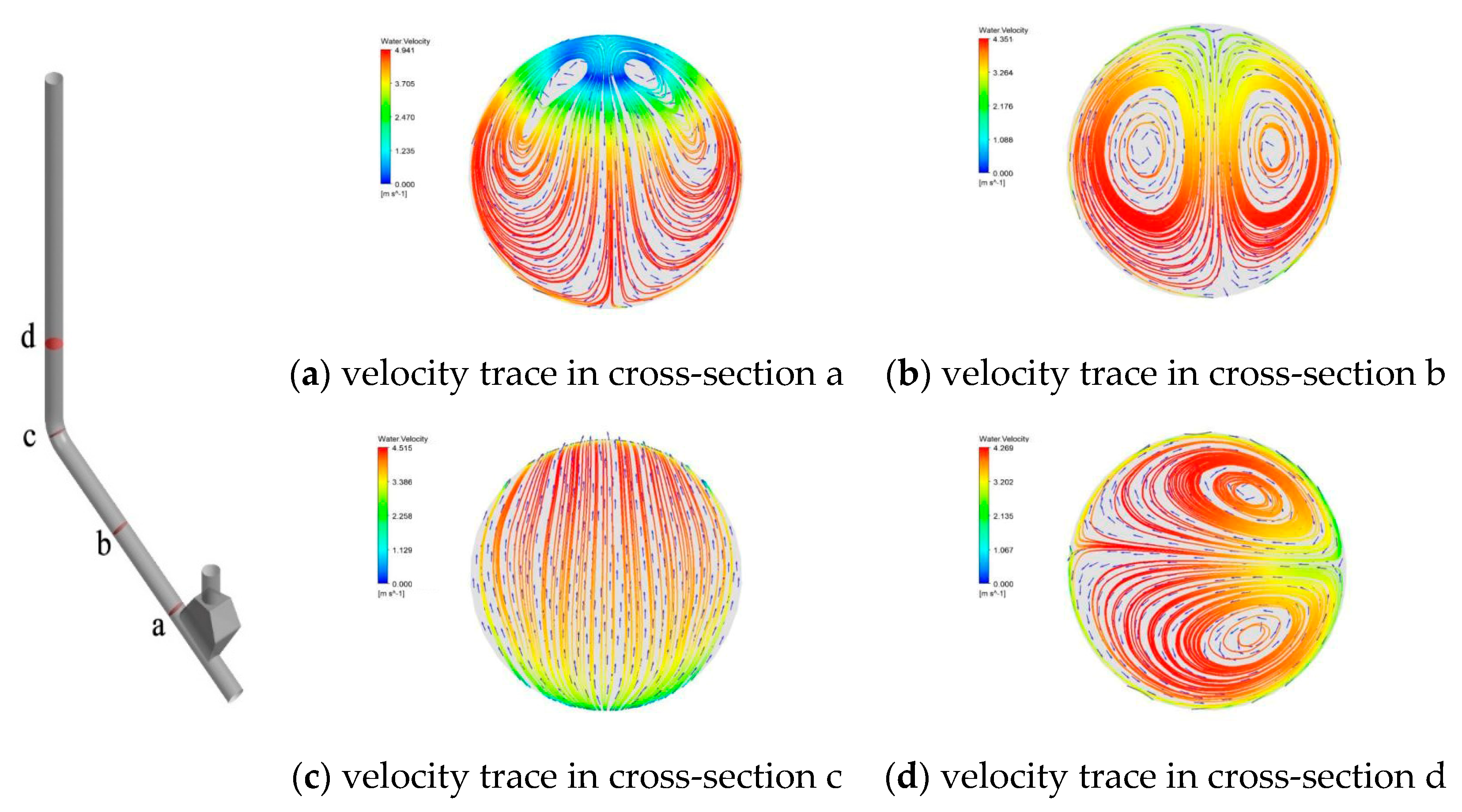
4.2.2. Secondary Flow
5. Conclusions
Author Contributions
Funding
Acknowledgments
Conflicts of Interest
References
- Liu, Y.B.; Chen, J.Z.; Yang, Y.R. Numerical simulation of liquid-solid two-phase flow in slurry pipeline transportation. J. Zhejiang Univ. Eng. Sci. 2006, 40, 858–863. [Google Scholar]
- Kaushal, D.R.; Thinglas, T.; Tomita, Y.; Kuchii, S.; Tsukamoto, H. CFD modeling for pipeline flow of fine particles at high concentration. Int. J. Multiph. Flow. 2012, 43, 85–100. [Google Scholar] [CrossRef]
- Ravikumar, S.K.; Ziazi, R.M.; Chambers, F.W.; McNally, M.E.; Hoffman, R.M. Computational prediction of particle-laden slurry flow in a vertical pipe using Reynolds Stress Model. In Fluids Engineering Division Summer Meeting; American Society of Mechanical Engineers: New York, NY, USA, 2013; Volume 55560, p. V01CT20A008. [Google Scholar]
- Li, M.; He, Y.; Liu, Y.; Huang, C. Hydrodynamic simulation of multi-sized high concentration slurry transport in pipelines. Ocean Eng. 2018, 163, 691–705. [Google Scholar] [CrossRef]
- Messa, G.V.; Malavasi, S. A CFD-based method for slurry erosion prediction. Wear 2018, 398, 127–145. [Google Scholar] [CrossRef]
- Qiang, Z. Simulation Analysis of Sinking Process of Particles Falling into Water Based on Coupled CFD-DEM. Master’s Thesis, Jilin University, Jilin, China, 2014. [Google Scholar]
- Parsi, M.; Kara, M.; Agrawal, M.; Kesana, N.; Jatale, A.; Sharma, P.; Shirazi, S. CFD simulation of sand particle erosion under multiphase flow conditions. Wear 2017, 376, 1176–1184. [Google Scholar] [CrossRef]
- Huang, S.; Shu, Y.L.; Zhou, J.J.; He, D.P.; Peng, T.Y. Numerical simulation for solid-liquid two-phase flow in discharge pipeline and flange connection by CFD-DEM coupling. Hydromechatronics Eng. 2017, 12, 1–6. [Google Scholar]
- Kannojiya, V.; Deshwal, M.; Deshwal, D. Numerical Analysis of Solid Particle Erosion in Pipe Elbow. Mater. Today Proc. 2018, 5, 5021–5030. [Google Scholar]
- Cundall, P.A.; Strack, O.D.L. A discrete numerical model for granular assemblies. Géotechnique 1979, 29, 47–65. [Google Scholar] [CrossRef]
- Chen, X.; Zhong, W.; Zhou, X.; Jin, B.; Sun, B. CFD–DEM simulation of particle transport and deposition in pulmonary airway. Powder Technol. 2012, 228, 309–318. [Google Scholar] [CrossRef]
- Capecelatro, J.; Desjardins, O. An Euler–Lagrange strategy for simulating particle-laden flows. J. Comput. Phys. 2013, 238, 1–31. [Google Scholar] [CrossRef]
- Park, K.M.; Yoon, H.S.; Kim, M.I. CFD-DEM based numerical simulation of liquid-gas-particle mixture flow in dam break. Commun. Nonliner Sci. 2018, 59, 105–121. [Google Scholar] [CrossRef]
- Huang, S.; Su, X.; Qiu, G. Transient numerical simulation for solid-liquid flow in a centrifugal pump by DEM-CFD coupling. Eng. Appl. Comp. Fluid. 2015, 9, 411–418. [Google Scholar] [CrossRef]
- Kloss, C.; Goniva, C.; Hager, A.; Amberger, S.; Pirker, S. Models, algorithms and validation for opensource DEM and CFD–DEM. Prog. Comput. Fluid Dyn. 2012, 12, 140–152. [Google Scholar] [CrossRef]
- Blais, B.; Bertrand, O.; Fradette, L.; Bertrand, F. CFD-DEM simulations of early turbulent solid–liquid mixing: Prediction of suspension curve and just-suspended speed. Chem. Eng. Res. Des. 2017, 123, 388–406. [Google Scholar] [CrossRef]
- Uzi, A.; Levy, A. Flow characteristics of coarse particles in horizontal hydraulic conveying. Powder Technol. 2018, 326, 302–321. [Google Scholar] [CrossRef]
- Park, Y.C.; Yoon, C.H.; Lee, D.K.; Kwon, S.K. Experimental Studies on Hydraulic Lifting of Solid-liquid Two-phase Flow. Ocean Polar Res. 2004, 26, 647–653. [Google Scholar] [CrossRef]
- Chen, C.G.; Yang, Y.; Tang, D.S.; Jin, X.; Xiao, H. Study on the settling regularity of solid particles in vertical pipelines. Int. J. Sediment Res. 2010, 4, 16–21. [Google Scholar]
- Wang, Y.; Yang, N.; Jin, X. Study on the Motion Path of Solid Particle in Vertical Pipeline. Jinshu Kuangshan/Met. Mine 2011, 40, 36–39. [Google Scholar]
- Vittorio Messa, G.; Malavasi, S. Numerical prediction of particle distribution of solid-liquid slurries in straight pipes and bends. Eng. Appl. Comput. Fluid Mech. 2014, 8, 356–372. [Google Scholar] [CrossRef][Green Version]
- Wijk, J.M.V.; Talmon, A.M.; Rhee, C.V. Stability of vertical hydraulic transport processes for deep ocean mining: An experimental study. Ocean Eng. 2016, 125, 203–213. [Google Scholar] [CrossRef]
- Ekambara, K.; Sanders, R.S.; Nandakumar, K.; Masliyah, J.H. Hydrodynamic Simulation of Horizontal Slurry Pipeline Flow Using ANSYS-CFX. Ind. Eng. Chem. Res. 2009, 48, 8159–8171. [Google Scholar] [CrossRef]
- Zhang, H.; Chen, L.; Xie, R.; Liu, X.; Zheng, X.; Shang, Z. Numerical simulation of solid-liquid two-phase steady flow in horizontal pipe. J. Chem. Ind. Eng. Soc. China 2009, 5, 1162–1168. [Google Scholar]
- Capecelatro, J.; Desjardins, O. Eulerian–Lagrangian modeling of turbulent liquid–solid slurries in horizontal pipes. Int. J. Multiph. Flow 2013, 55, 64–79. [Google Scholar] [CrossRef]
- Messa, G.V.; Malin, M.; Malavasi, S. Numerical prediction of fully-suspended slurry flow in horizontal pipes. Powder Technol. 2014, 256, 61–70. [Google Scholar] [CrossRef]
- Singh, J.P.; Kumar, S.; Mohapatra, S.K. Modelling of two phase solid-liquid flow in horizontal pipe using computational fluid dynamics technique. Int. J. Hydrogen Energy 2013, 42, 20133–20137. [Google Scholar] [CrossRef]
- Messa, G.V.; Malavasi, S. Numerical prediction of dispersed turbulent liquid-solid flows in vertical pipes. J. Hydraul. Res. 2014, 52, 684–692. [Google Scholar] [CrossRef]
- Kaushal, D.R.; Kumar, A.; Tomita, Y.; Kuchii, S.; Tsukamoto, H. Flow of Bi-modal Slurry through Horizontal Bend. Kona Powder Part. J. 2017, 34, 258–274. [Google Scholar] [CrossRef]
- Oka, Y.I.; Okamura, K.; Yoshida, T. Practical estimation of erosion damage caused by solid particle impact. Wear 2005, 259, 95–101. [Google Scholar] [CrossRef]
- Cao, B.; Xia, J.X.; Hei, P.F.; Liu, X. Study on the Movement State of Coarse-grain during Hydraulic Transportation in Pipeline of Complex Spatial Morphology. Min. Met. Eng. 2012, 2, 5–10. [Google Scholar]
- Chen, J.K.; Wang, Y.S.; Li, X.F.; He, R.Y.; Han, S.; Chen, Y.L. Erosion prediction of liquid-particle two-phase flow in pipeline elbows via CFD–DEM coupling method. Powder Technol. 2015, 282, 25–31. [Google Scholar] [CrossRef]
- Peng, W.; Cao, X. Numerical simulation of solid particle erosion in pipe bends for liquid–solid flow. Powder Technol. 2016, 294, 266–279. [Google Scholar] [CrossRef]
- Masanobu, S.; Takano, S.; Fujiwara, T.; Kanada, S.; Ono, M.; Sasagawa, H. Study on Hydraulic Transport of Large Solid Particles in Inclined Pipes for Subsea Mining. J. Energy Resour. Technol. 2017, 139. [Google Scholar] [CrossRef]
- Zhu, H.P.; Zhou, Z.Y.; Yang, R.Y.; Yu, A.B. Discrete particle simulation of particulate systems: Theoretical developments. Chem. Eng. Sci. 2007, 62, 3378–3396. [Google Scholar] [CrossRef]
- Chu, K.W.; Chen, J.; Yu, A.B. Applicability of a coarse-grained CFD–DEM model on dense medium cyclone. Min. Eng. 2016, 90, 43–54. [Google Scholar] [CrossRef]
- Alletto, M.; Breuer, M. Prediction of turbulent particle-laden flow in horizontal smooth and rough pipes inducing secondary flow. Int. J. Multiph. Flow. 2013, 55, 80–98. [Google Scholar] [CrossRef]
- Jia, M.; Yan, C.; Song, J.; Wei, Y.; Zhou, F.; Sun, L.; Wang, D. Experimental and numerical study of secondary flow in a T-type bend of a CFB riser. Chem. Eng. J. 2018, 334, 1222–1232. [Google Scholar] [CrossRef]


| Name | Model | Parameters |
|---|---|---|
| Centrifugal pump | ISG 50-160 (I) A | The rated power is 3 kW, the rated flow is 29 m3/h, the lift is 16 m, the rotational speed is 2900 r/min and the corrosion-resistant mechanical seal is adopted. |
| Electromagnetic flowmeter | ZJLDG-50 | The nominal diameter is 50 mm, the working range is 0.7–106 m3/h, the working pressure is 1.6 MPa, the working temperature is under 80 °C, the electrode is made of 316 L stainless steel and the lining is polyurethane. |
| Frequency converter | Emerson-Enydrive TD3000 | The suitable motor power is below 7.5 kW, the rated voltage is 380 V, the output frequency is 0–400 Hz, four digit digital display, with Chinese and English LCD display, the installation mode is wall mounted. |
| High speed camera | Phantom VEO 410 L | The full frame resolution is 1280 × 800. The full frame shooting rate is 5200 frames/S. In this state, 9.6 s can be recorded. The minimum exposure time is 1 μs, the maximum shooting speed is 600,000 frames/s, the number of pixels is 1,024,000, and the pixel size is 20 μm. |
| Forces and Torques | Type | Formula |
|---|---|---|
| Normal forces | Contact | |
| Damping | ||
| Tangential forces | Contact | |
| Damping | ||
| Particle-fluid forces | Pressure gradient force | |
| Fluid drag force | ||
| Torques | Tangential | |
| Rolling | ||
| Where:, , , , , , . | ||
| Trial Simulation Conditions | Mesh Quality | Grid Quantity | Average Fluid Velocity at Outlet (m/s) |
|---|---|---|---|
| Particle-inlet 0.5 m/s, Particle | Coarse | 50,778 | 2.4826 |
| diameter 5 mm | Medium | 83,488 | 2.4953 |
| Generation rate 0.5 kg/s | Fine | 133,952 | 2.4999 |
| Water-inlet 2.0 m/s, Pressure outlet | Finest | 277,966 | 2.5001 |
| Case | Working Conditions | vp (m/s) | vf (m/s) |
|---|---|---|---|
| 1 | Low (20 Hz) | 0.76 | 0.55 |
| 2 | Medium (30 Hz) | 1.28 | 1.27 |
| 3 | High (40 Hz) | 1.83 | 2.00 |
| Poisson’s Ratio | Shear Modulus (Pa) | Density (kg/m3) | |
|---|---|---|---|
| Y-shaped elbow | 0.40 | 9.89 × 10⁸ | 7800 |
| Particle | 0.22 | 2.13 × 10⁷ | 2000 |
| Case | Simulation | Experiment |
|---|---|---|
| Case 1 (20 HZ) vp > vf vp = 0.76 m/s vf = 0.55 m/s |  |  |
| Case 2 (30 HZ) vp ≈ vf vp = 1.28 m/s vf = 1.27 m/s |  |  |
| Case 3 (40 HZ) vp < vf vp = 1.83 m/s vf = 2.00 m/s |  |  |
© 2020 by the authors. Licensee MDPI, Basel, Switzerland. This article is an open access article distributed under the terms and conditions of the Creative Commons Attribution (CC BY) license (http://creativecommons.org/licenses/by/4.0/).
Share and Cite
Hu, Q.; Zou, L.; Lv, T.; Guan, Y.; Sun, T. Experimental and Numerical Investigation on the Transport Characteristics of Particle-Fluid Mixture in Y-Shaped Elbow. J. Mar. Sci. Eng. 2020, 8, 675. https://doi.org/10.3390/jmse8090675
Hu Q, Zou L, Lv T, Guan Y, Sun T. Experimental and Numerical Investigation on the Transport Characteristics of Particle-Fluid Mixture in Y-Shaped Elbow. Journal of Marine Science and Engineering. 2020; 8(9):675. https://doi.org/10.3390/jmse8090675
Chicago/Turabian StyleHu, Qiong, Li Zou, Tong Lv, Yingjie Guan, and Tiezhi Sun. 2020. "Experimental and Numerical Investigation on the Transport Characteristics of Particle-Fluid Mixture in Y-Shaped Elbow" Journal of Marine Science and Engineering 8, no. 9: 675. https://doi.org/10.3390/jmse8090675
APA StyleHu, Q., Zou, L., Lv, T., Guan, Y., & Sun, T. (2020). Experimental and Numerical Investigation on the Transport Characteristics of Particle-Fluid Mixture in Y-Shaped Elbow. Journal of Marine Science and Engineering, 8(9), 675. https://doi.org/10.3390/jmse8090675