1. Introduction
Modelling shoreline change is one of the major contemporary challenges facing coastal communities around the world. Nearly one-quarter of the global population live within 100 km of the coastline, with these regions becoming ever more densely populated [
1]. When considering that the evidence suggests that sea level rise is accelerating [
2,
3], it is more than likely that the scale of the problem will only intensify. It is imperative that scientists and coastal managers develop effective tools to forecast coastal change, such that these regions can be safely and efficiently managed.
There is no single adopted method for modelling coastal processes. More complicated process-based models (for example XBeach [
4]) can be very demanding computationally and require parameterisation of a large number of physical processes. Equilibrium models by contrast are much simpler, linking hydrodynamic forcing directly to shoreline change and thus omitting many of the intricate physical processes involved, which allows for faster computation [
5]. This in turn opens the door to longer-term forecasting on seasonal to decadal timescales [
6]. These are the timeframes that are of most interest to coastal managers, and at which more complicated models are yet to produce accurate forecasts [
7]. Despite their simplicity and omission of several significant processes (such as tides), equilibrium models have also been shown to perform well over a range of sites globally [
8]. The importance of matching model complexity with the spatial and temporal scale of the problem and producing readily interpretable quantitative results is paramount [
9]. Models of reduced complexity (such as equilibrium models) are well suited to forecasting on seasonal/annual timescales and exhibit a favourable balance between accuracy and computational load that lends itself to ensemble forecasting and probabilistic predictions, as demonstrated by Davidson et al. [
6]. This allows for rigorous risk assessments to be produced that can then contribute to quantifiable economic arguments in shoreline management [
10].
It has been known for some time that knowledge of antecedent conditions is vital in predicting future beach states [
11]. This principle is common to many equilibrium models, which have previously been shown to perform well when predicting shoreline change on cross-shore dominated coastlines (for example [
12]). ShoreFor is derived from a similar baseline of assumptions, with rate of change of shoreline position proportional to the ‘state of disequilibrium’—the difference between the instantaneous and the antecedent wave climate [
13]. Simply put, when the current wave climate is more energetic than the preceding conditions the model predicts erosion, and conversely in the opposite case beach accretion is predicted. The model is also sensitive to incident wave power (P), with stronger shoreline responses predicted as power increases. For a full derivation, the reader is referred to Davidson et al. [
13]. A slight variant on ShorFor is employed in this work; where Davidson et al. [
6] used disequilibrium in dimensionless fall velocity, this study looks at wave breaker height only (H
b) and considers the disequilibrium in H
b1.5, with a linear trend term included as per Davidson et al. [
13].
Using the ShoreFor model, Davidson et al. [
6] devised a methodology to calculate the return periods of erosion events (and subsequent recoveries). The study considered two sites, the seasonally dominated Perranporth in the UK, and storm dominated Narrabeen in Australia. During the calibration phase the model showed good skill in producing validation hindcasts at each site (correlation coefficients of 0.98 and 0.89, respectively). Next, a Monte-Carlo simulation based on the local wave climate statistics at each site was used to generate 10
3 synthetic wave sequences to drive the model. The resulting set of shoreline forecasts were then used to derive the return periods of the storm erosion events via Generalised Extreme Value (GEV) analysis [
6]. One assumption embedded in this approach is that the historic wave data used to generate the synthetic waves are representative of likely future conditions, therefore interannual variability and underlying trends in wave climate are ignored [
6]. Suggestions were proposed—what if the relevant climate mode were known for the forecast period? Climate patterns such as North Atlantic Oscillation (NAO) are known to influence wave climate [
14], therefore if the index was known for the coming season a refined set of more relevant wave statistics could be used to run the model [
6].
In the northeast Atlantic (NEA), the NAO is one of the dominant modes of atmospheric variability and its influence on the region’s climate is well known [
15,
16]. For the purpose of this study, it is the relationship between the NAO and the nearshore wave climate at Perranporth that is of interest. The relevance of the NAO is greatest during winter months, as this is when the atmosphere is most dynamic, with greater scope for large-amplitude perturbations to develop [
17]. Bauer et al. [
18] found good correlation between the winter averaged significant wave height (H
s) and the winter NAO index (WNAO) in the NEA, although the timeseries of wave data used was only 12 years long. A 57 year hindcast performed by Dodet et al. [
19] found substantial interannual variability in H
s and wave period (T
p) in the NEA over the last 60 years, particularly during the months December–March. Furthermore, at northern latitudes they found a strong positive correlation between the WNAO and winter averaged H
s and T
p (r = 0.86 and r = 0.75, respectively, at 55° N, for example). When attempting to model shoreline change, it is the impact of the waves on the coastline that is important. Bromirski and Cayan [
20] recognised that the rate of energy transfer by waves is a key driver of coastal processes, and subsequently chose to investigate the link between wave power (P) and the WNAO in the NEA. Strong links were found over monthly and interdecadal timescales.
The obvious benefit in being able to predict the NAO (and in particular the WNAO) as a method to forecast wave conditions was highlighted as a recurring theme in the literature, and forms part of the motivation for this research. Although other indices such as the Scandinavian pattern (SCAN) and the East Atlantic pattern (EA) are known to influence Atlantic climate [
14], the NAO’s predictability has driven its inclusion in this study. Scaife et al. [
21] showed that with lead times of the order of one month, an ensemble forecast of WNAO (December–February) could be produced using the Met Office’s GloSea5 forecast model with reasonable skill (correlation coefficient r = 0.62 using 24 ensemble members). Inspired by the societal value of longer-range climate prediction, Dunstone et al. [
22] have increased this forecast range to over one year (correlation coefficient r = 0.42 using 40 ensemble members) using the Met Office’s DePreSys3 forecast model. This work is encouraging, as it suggests that a priori knowledge of climate indices is indeed realistic.
In western Europe, the winter of 2013/14 is associated with the extreme levels of erosion observed around its exposed Atlantic-facing coastlines, caused by an extraordinary sequence of high-energy storms [
23]. The established climate patterns such as the NAO failed to accurately represent the increased levels of wave energy observed that winter, leading to the formation of a new index by Castelle et al. [
24] called the ‘Western Europe Pressure Anomaly’ (WEPA). WEPA was explicitly designed to represent the wave climate incident on Europe’s Atlantic coastlines, and Castelle et al. [
24] showed that it outperformed the other established indices in explaining wave activity south of 52° N. Therefore, it is the most relevant index to the site location (Perranporth beach is approximately 50° N) and will be included in this study.
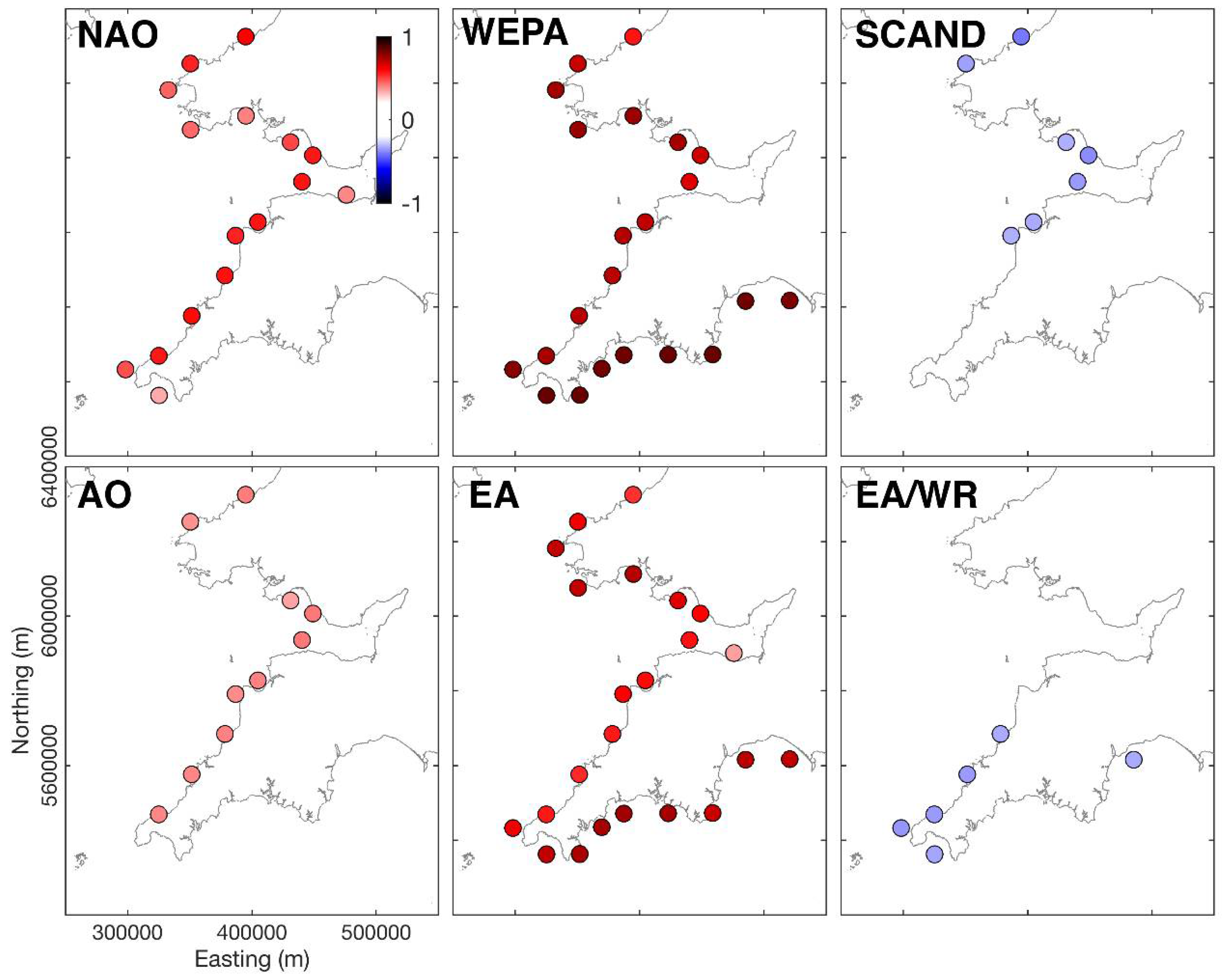
To add further weight to the decision to include only the WEPA and NAO indices in this work,
Figure 1 (data taken from Scott et al. [
25]) shows the correlation between winter averaged wave power in the southwest UK and six of the leading climate indices applicable to the NEA. The SCAND and East Atlantic Western Russian (EA/WR) patterns show weak negative correlation with wave power, with the Arctic Oscillation (AO) showing a similar pattern of correlation to NAO and the EA tracking WEPA. Crucially, the NAO and WEPA outperform the AO and EA respectively in terms of correlation in this region. Therefore, they are the two most influential indexes at the test site and inclusion of any others would not add any extra insight to this study.
There is existing research that has linked climate patterns to shoreline change. For example, Robinet et al. [
26] showed that much of the shoreline variability at Truc Vert (southwest France) could be explained by a model composed of atmospheric circulation patterns or ‘weather regimes’—some of which coincide with positive and negative modes of NAO. Further to this, it has been shown more generally that beach recovery rates on the Atlantic coast of Europe are strongly linked with climate patterns such as the WEPA and NAO [
27]. This work aims to go one step further and use the NAO and WEPA climate patterns to directly influence the composition of the synthetic waves used to drive the model. In doing so, it will be possible to deduce whether more skilful shoreline predictions are possible if climate patterns are known beforehand. Initially, the synthetic wave creating function used to drive ShoreFor was adapted such that it could be informed by climate index information. This was then used to forecast shoreline change at Perranporth (
Figure 2) over eight winter seasons (December–March) from 2008/9 to 2015/16. Three runs were completed for each season—one informed by the NAO index, one by the WEPA index and a control run that used ‘uninformed’ wave forcing. The results from the three forecasts were then compared to survey data.
2. Materials and Methods
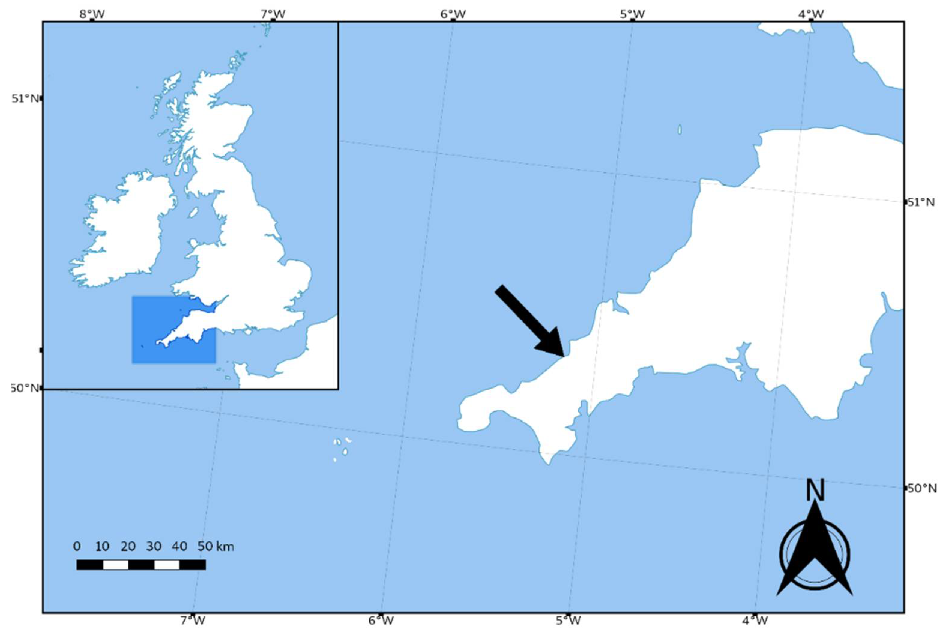
The site chosen for this study was Perranporth beach in the UK. Situated on the north coast of Cornwall (
Figure 2), it is approximately 3.5 km in length and faces west-northwest. It has a tidal range of 6.5 m (spring) and is seasonally dominated with winter periods generally associated with a higher frequency of energetic Atlantic swells arriving predominantly from the west [
6]. It is cross-shore dominated and thus typical of exposed, west-facing North Cornwall beaches. The beach state is seasonal and generally situated between low tide bar/rip and dissipative [
28] with a beach face gradient that is fairly flat, ranging between 0.015 and 0.025 [
29].
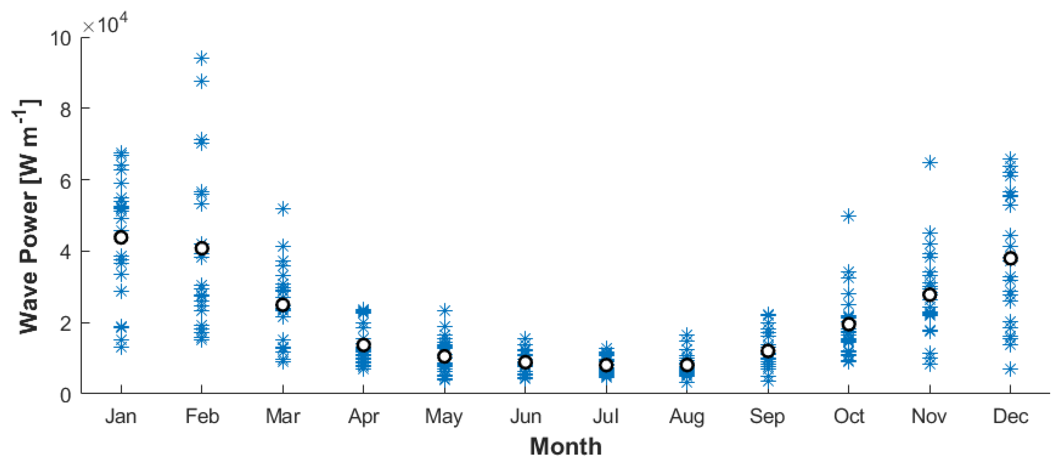
Figure 3 shows the significantly increased variability in wave power exhibited during winter (when compared to the summer) which is a critical factor in this study. The ShoreFor model has already been applied to this location with high skill (r = 0.98) [
6].
A 23 year-long timeseries of modelled (WWIII) hourly H
s and T
p data was obtained for a grid point off the coast of Perranporth (water depth of 35 m). From this, it was then possible to generate the key synthetic wave-forcing timeseries used to force the shoreline prediction model. Alongside this, a 12 year dataset (2006–2017) of cross-shore shoreline position at Perranporth was collected by GPS survey (Topographic RTK-GNSS), conducted monthly by the Coastal Processes Research Group at Plymouth University [
23]. For the climate indices, it was decided that monthly index values would be most appropriate for this study. This was for several reasons. Firstly, the synthetic waves driving ShoreFor are compiled on a monthly timescale, so with this in mind it seemed logical to inform the process on a monthly timeframe. Second, a month is sufficiently long to incorporate a full storm sequence and its corresponding effect on nearshore wave climate, but also sufficiently short such that variations in wave conditions throughout the four month long winter period (December–March) could be accommodated for (as opposed to with the seasonal indices for example). For NAO, following Martínez-Asensio et al. [
14], a 69 year timeseries (1950–2018) of monthly NAO index values (standardised by 1981–2010 climatology) were taken from the National Oceanic and Atmospheric Administration’s (NOAA) Climate Prediction Centre [
30]. For the WEPA index, a 74 year timeseries (1943–2016) of monthly values was acquired, as used by Castelle et al. [
24].
This study modifies the synthetic wave generation algorithm discussed in Davidson et al. [
6] to include the influence of selected climate indices. Davidson et al. [
6] generated multiple (10
3) random timeseries of the wave parameters used to force the model from an existing dataset of either measured or modelled wave statistics. The wave data were first sorted by month, and then each monthly subset rearranged. By selecting a month-long segment at random from each of the subsets in turn (12 times in total), a unique annual timeseries could be constructed that was seasonally representative. Because the time sequencing of each of the shuffled months was maintained, so were any storm periods in the data. This timeseries was then used to drive ShoreFor and produce an annual shoreline prediction, with this process repeated 10
3 times. It is the ensemble averaged shoreline which is presented in this contribution and compared with observations.
Two new versions of this algorithm were produced, one for the NAO-informed model and one for the WEPA-informed model. Firstly, the imported wave data were assigned the relevant monthly index value (NAO or WEPA) for the date recorded. After this it was possible to sort the data into three groups: Positive index months, negative index months, and finally the ‘full’ dataset as used in the existing ShoreFor wave forcing methodology by Davidson et al. [
6]. After this, the same randomising process that was previously applied to the single dataset was replicated twice more, once for the positive index months and once for the negative. This way, when constructing the synthetic waves on a month-by-month basis for each shoreline forecast, a new criterion could be added that checked the climate index value for the hindcast month in question to see if it was above or below a threshold value. If the index value was above the positive threshold, a random month-long sequence of data would be selected from the NAO+/WEPA+ dataset, with index values falling below the negative threshold leading to selection from the NAO−/WEPA− dataset. If the index value for the hindcast month did not breach the threshold in either direction, the full data pool was used to select a random segment of wave data. As in Davidson et al. [
6], all synthetic waves generated were unique.
This additional functionality was only applied to the wave-generating process during winter months (December–March), in which both NAO and WEPA are good indicators of wave conditions [
20,
24]. The key variables were the threshold values at which the wave climate statistics used were restricted to NAO+/WEPA+ or NAO−/WEPA− months only. If the threshold is too high then it is seldom breached, and the index-informed waves differ little from the uninformed waves. Too low, and the wave-generating process becomes overly responsive to small magnitude monthly index values, leading to unrepresentative synthetic waves based on excessively extreme wave climate data.
The correlation between the monthly mean wave power (P) at Perranporth and the monthly NAO and WEPA indices was calculated for the winter months (December–March) as well as the ‘summer’ (April–November) for comparison (
Table 1). The results show a much stronger relationship between monthly NAO and wave climate during winter, with negligible correlation between April and November. For WEPA, it is also the case that the monthly index is better correlated during winter. However, it still holds some relevance during the ‘summer’ months, although it should be mentioned that the significance of this is debatable as ‘summer’ wave conditions are generally less powerful and less variable (see
Figure 3). These findings support the existing literature and further vindicate the decision to restrict the climate-informed functionality from December to March.
Figure 4 illustrates the comparison of monthly mean wave power for Perranporth between positive and negative NAO/WEPA months. The effect of a positive monthly index value on P is clear, with both NAO+ and WEPA+ months associated with more energetic conditions (the opposite being true for negative index values). What is also noticeable is the generally stronger signal between WEPA and P when compared with NAO, which itself has particularly little influence on P during January and March.
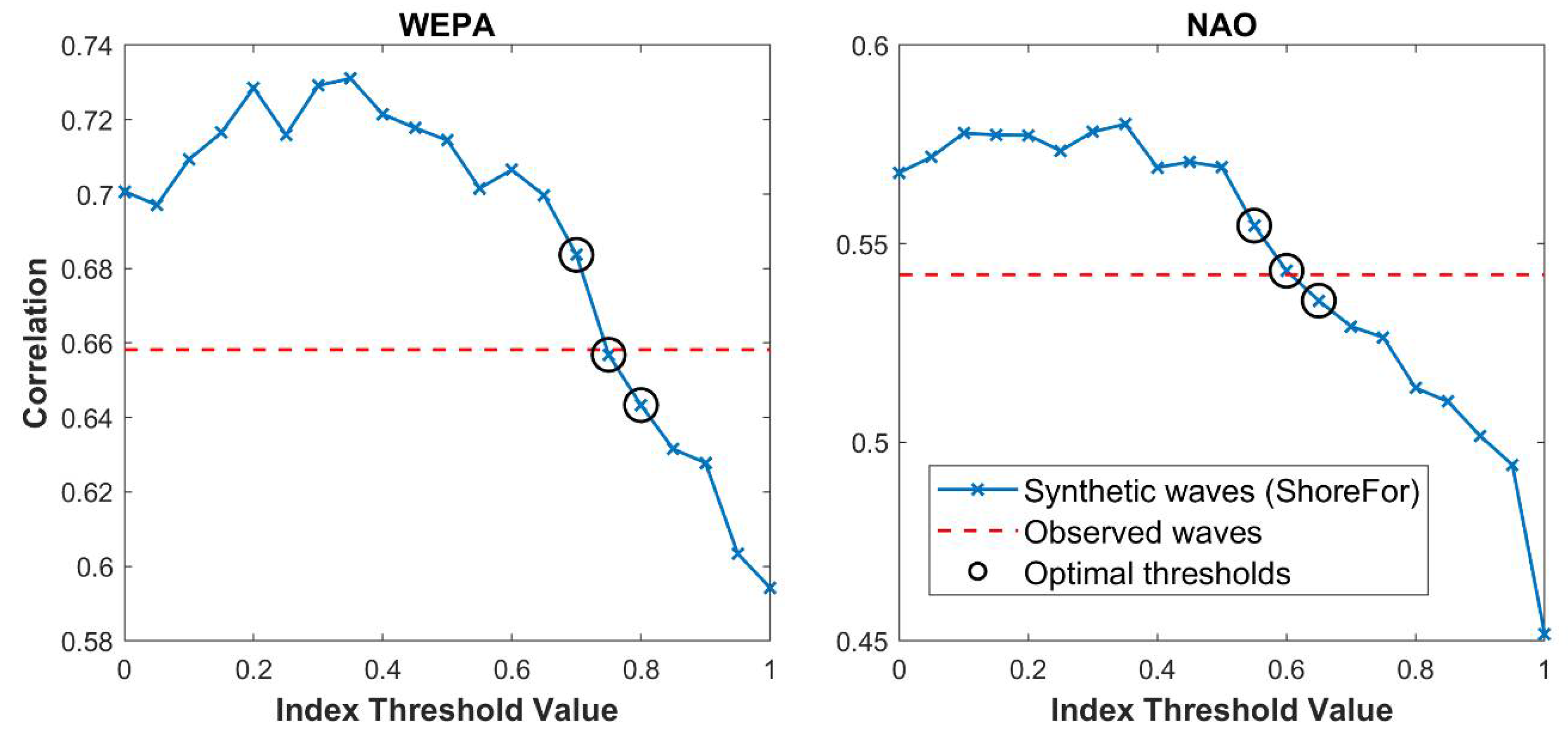
To test the new wave forcing methodology, it was first essential to tune the threshold index values used at which the function creating the synthetic waves would draw data from positive index or negative index months only. This was performed by analysing the correlation between the monthly average wave power of the synthetic waves generated and the corresponding monthly climate index as the threshold value was changed (performed separately for both NAO and WEPA). The goal was to find the thresholds at which the synthetic waves generated exhibited a similar correlation with the climate indices to that observed from the historic data, such that the NAO-informed and WEPA-informed wave forcing of ShoreFor was as representative of real conditions as possible.
The maximum dataset was used in each case such that the monthly climate index timeseries and historic wave data overlapped. For NAO this was December 1994 to March 2017, and for WEPA it was December 1994 to March 2016. The threshold value was varied between 0 and 1 at 0.05 increments, resulting in 21 runs for each climate index (
Figure 5). Three thresholds were chosen for both NAO and WEPA such that the correlation exhibited by the synthetic waves and the indices was most representative. These were 0.55, 0.60 and 0.65 for NAO, and 0.70, 0.75 and 0.80 for WEPA.
Following the correlation analysis full model runs were performed for each threshold value for each index, with the best performing threshold for each chosen as the final parameterisation. For NAO, as none of the index values for the winter months fell in the 0.55–0.65 range for the entire hindcast period, all three parametrisations deliver exactly the same forecast methodology. Therefore, the final selection was arbitrary and a threshold value of 0.60 was chosen, with the version of ShoreFor using this wave forcing methodology hereafter denoted as ‘SF-NAO’. For WEPA, whilst the differences were small the threshold value delivering the best results (i.e., smallest errors) was 0.70, with this version of ShoreFor hereafter denoted ‘SF-WEPA’. The uninformed ShoreFor model is referred to as ‘SF-Uninf’.
With both the NAO-informed and WEPA-informed models parameterised, the next step was to compare the winter storm response forecasts of each to the uninformed model predictions, as well as to each other. The hindcast seasons were selected such that both climate indices had complete monthly timeseries overlapping and that the shoreline dataset had at least three measurements taken for the chosen winter. Eight winter seasons met this requirement and were selected (from 2008/9 until 2015/16). Each season was run from 1 December until 1 April, encompassing the full period during which the wave statistics used to force the model could be informed by the relevant climate index. It would of course be possible to extend the runs, either for the full year or even to produce multi-annual forecasts. However, it was decided to restrict the forecast period to the months during which the NAO and WEPA hold relevance over the wave climate, so as to give a clearer comparison between the three wave forcing methodologies. In addition to this, it is during the winter that Perranporth usually experiences the most dramatic changes in shoreline [
6] and as such should be the most interesting and relevant period in which to compare the forecasts. The real wave data for each forecast period were removed during the synthetic wave creation for each run to ensure a fair test of the three model runs, as per Davidson et al. [
6]. However, all of the available data were used to calibrate the model free parameters in ShoreFor. Normally during a hindcast it would be necessary for the data within the forecast period to be removed prior to the calibration process. Nevertheless, the aim of this study was to assess the impact of informing ShoreFor with climate indices specifically, so because the absolute performance of the model was not being assessed it was decided to use all available data to tune the parameters and keep this consistent for all model runs.
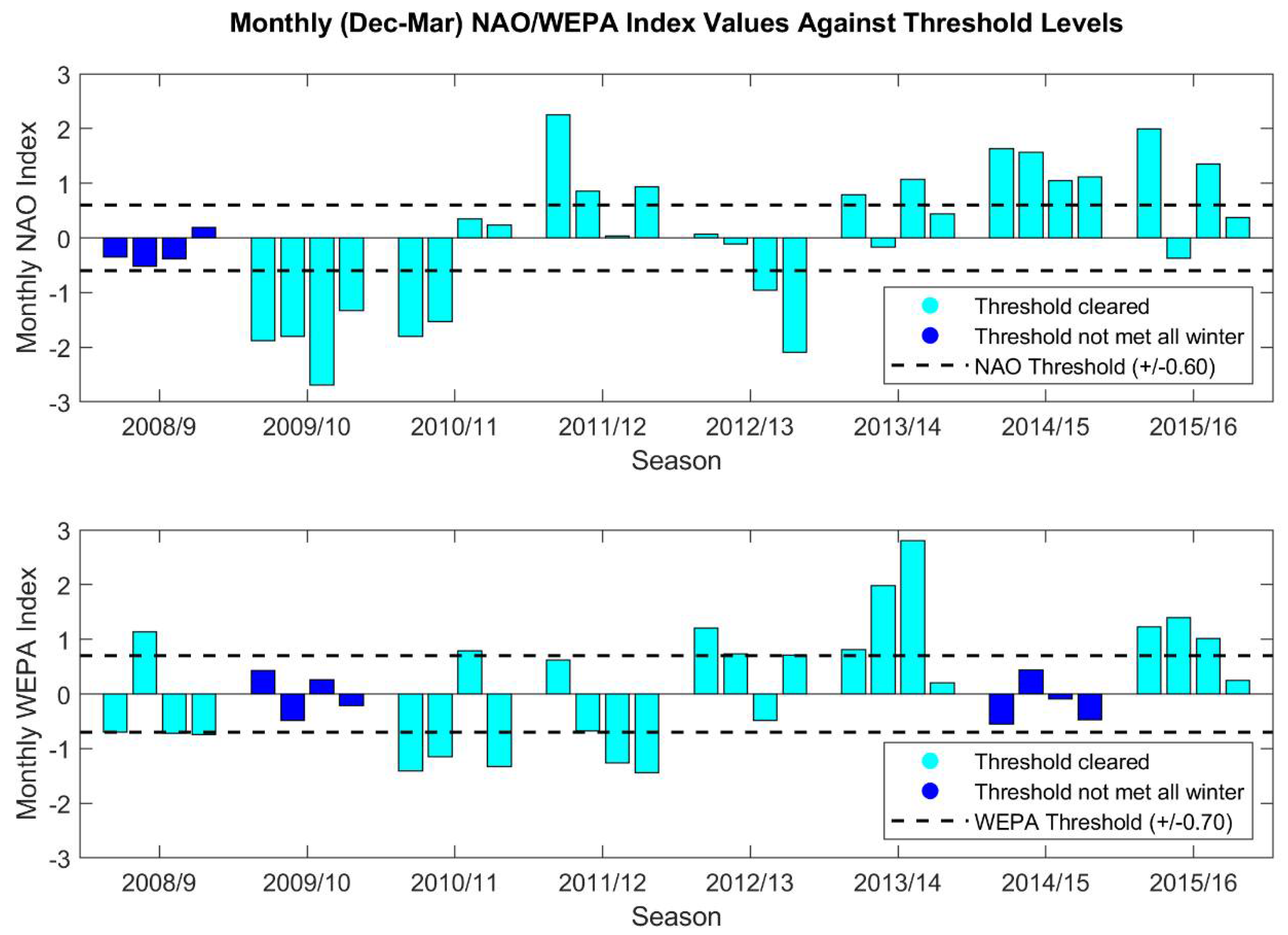
For the winters during which the thresholds are not breached in any of the four months (see
Figure 6), the climate-informed model delivers an identical wave forcing methodology to SF-Uninf, leading to identical forecast results. These are omitted from the forecast plots in the results. However, when comparing the overall skill of SF-NAO and SF-WEPA for the full hindcast period, these seasons are still included in the calculation. This is because if the climate-informed models were operational, then it is the case that during winter seasons where monthly index values were not of a sufficient magnitude to breach the threshold level the wave forcing methodology would fall back on that of SF-Uninf, using all the available wave data. Therefore, for this calculation the results from SF-Uninf are substituted in for those seasons.
Two statistical measures were used to compare the relative skill of all three models for each winter forecast. Here, only the mean shoreline was considered for each wave forcing methodology (each model run produces 10
3 shorelines). Root mean square error (RMSE) was used to quantify the difference between the forecasts and the survey points each winter, and is defined as:
where
n is the number of surveys taken, with
oi representing the observation—in this case, the surveyed shoreline—and
mi representing the corresponding model output. The surveyed shoreline was recalibrated to zero at the start of the forecast (1 December) by interpolating the two survey points either side of the start date (the model forecast automatically starts with the shoreline at zero). The ‘skill score’, or ‘index of agreement’ is a dimensionless measure of a models predictive capability, and takes into account both the error in model output as well as how well the variability predicted by the model matches that of the observations [
31]. The version used in this study was taken from Willmott, Robeson and Matsuura [
31] and is defined as:
where, as with RMSE,
n is the number of surveys taken that winter,
oi is the surveyed shoreline,
mi is the corresponding modelled shoreline and
ō the mean of the surveys. The skill score ranges between 1 and 0, with 1 indicating a perfect prediction and 0 demonstrating complete disagreement [
31]. In order to confirm the statistical significance of the differences between the three forecasts, it was necessary to consider the full set of underlying predicted shorelines (10
3 for each wave forcing methodology) and compare the distributions of each model output at every survey point. This was to ensure that the new wave forcing methods employed by both SF-NAO and SF-WEPA produced distinct results from both each other as well as SF-Uninf. Due to the distribution of these shorelines being non-parametric, a Wilcoxon rank-sum test (or Mann-Whitney U test) was used.
3. Results
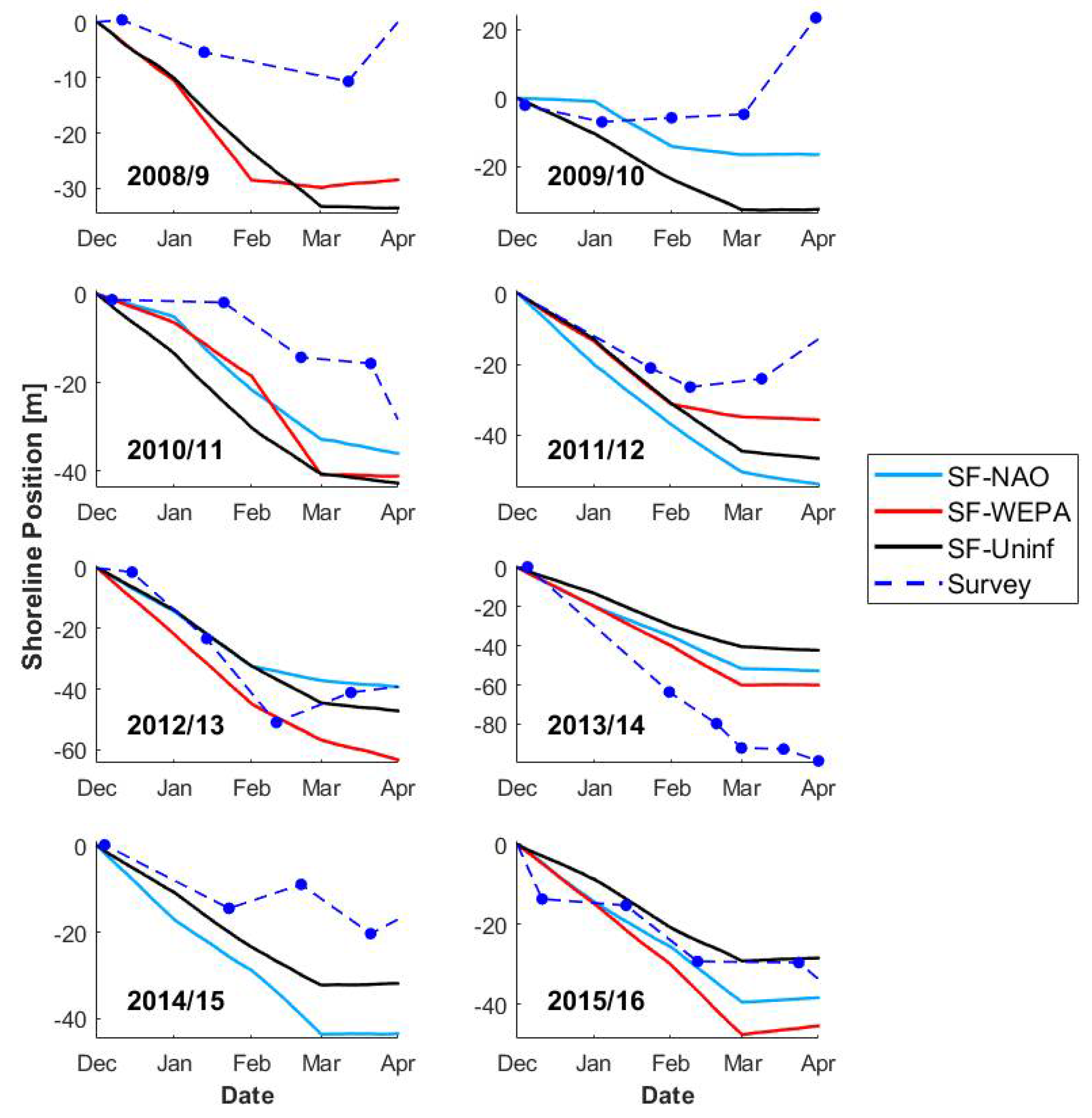
Figure 7 shows comparisons between the SF-NAO, SF-WEPA and SF-Uninf forecasts. For the seasons during which the index thresholds were not breached, the respective climate-informed forecasts were not included due to being identical in methodology to SF-Uninf (2008/9 for NAO, 2009/10 and 2014/15 for WEPA). The RMSE and skill score results for SF-NAO and SF-WEPA are shown in
Figure 8 as differences between the corresponding model score and the SF-Uninf score for each winter season. Bars above the line indicate improvements in model performance over the uninformed ShoreFor forecast, with bars below the line indicating worse scores.
The results are fairly mixed for SF-NAO. A clear improvement on SF-Uninf was made in the 2009/10, 2010/11, and the 2013/14 seasons, with reductions in RMSE of 10.04, 6.70 and 8.70 m and increases in skill score of 0.02, 0.13 and 0.09, respectively (
Figure 8). The worst performance was during the 2011/12 and 2014/15 winters. Here, not only did SF-NAO fail to improve on SF-Uninf but the errors were actually significantly worse, with RMSE scores of 5.61 m and 7.51 m higher and skill scores of 0.04 and 0.15 lower, respectively. Both the 2012/13 and 2015/16 forecasts show small performance differences between SF-NAO and SF-Uninf.
SF-WEPA appears to show a more consistent reduction in error over SF-Uninf than SF-NAO. The seasons during which SF-WEPA offers a clear improvement over SF-Uninf as seen from the plots (
Figure 7) are backed up by significant reductions in RMSE (3.56, 5.48 and 15.17 m) and increases in skill score (0.08, 0.14, 0.16), as was the case with SF-NAO. However, during the other three seasons where an obvious improvement is not clear from the forecast plots (2008/9, 2012/13, 2015/16) the magnitude of the difference in error between SF-WEPA and SF-Uninf is typically small (RMSE values of −1.50, +3.01, and +4.47 m and skill scores of +0.02, −0.02, −0.08, respectively, illustrated by
Figure 8). This suggests that informing the synthetic wave creation with the WEPA index could deliver a meaningful improvement over ShoreFor’s existing wave forcing methodology, as the results show large reductions in error interspersed with small increases in error. This contrasts with SF-NAO which produced notably worse forecasts to SF-Uninf as well as improvements.
3.1. Summary of Model Performance
In order to comprehensively assess any potential improvements on SF-Uninf by either SF-NAO or SF-WEPA, it was necessary to summarise their performance over the full hindcast period. This was performed by taking the average RMSE and skill score over the eight winters, substituting the respective SF-Uninf values in for those seasons during which the thresholds were not breached (2008/9 for SF-NAO, 2009/10 and 2014/15 for SF-WEPA). This was done to simulate operationalisation of the climate-informed models, as during those winters where the relevant index did not breach the threshold value the wave-forcing methodology would revert to that employed by SF-Uninf (although it is important to caveat here that current climate index forecasting capabilities are limited to seasonal index values only, not monthly). The results are summarised in
Table 2.
SF-NAO has the same skill score as SF-Uninf but a slightly better RMSE (1.31 m lower), suggesting that this wave forcing methodology offers a marginal improvement. SF-WEPA shows a much clearer reduction in error, with the average RMSE 2.28 m lower and skill score 0.03 higher, suggesting that a more significant improvement on SF-Uninf is possible when using this wave forcing methodology.
3.2. Statistical Significance of Results
The assessment of the statistical significance of the difference between each of the forecasts was performed on every survey date. For the vast majority of the surveys the
p-values are less than 0.001, indicating a good degree of confidence in the uniqueness of the three wave forcing methods. In general, the few
p-values greater than 0.001 were in the earlier surveys (i.e., the beginning of the forecasts) and can be accounted for either by index thresholds not being breached, or when comparing SF-WEPA to SF-NAO, thresholds being breached in the same direction. For a full set of results, see
Table A1,
Table A2 and
Table A3 in
Appendix A.
4. Discussion
Overall, both of the new wave forcing methodologies delivered forecasts with a range of error variability, both better than or worse than SF-Uninf at times. The key advantage in SF-WEPA over SF-NAO was that in general SF-WEPA offered larger reductions in error versus SF-Uninf interspersed with smaller increases (
Figure 8), reducing overall RMSE and increasing overall skill score by a greater degree, respectively (
Table 2). The mixed results from SF-NAO and more consistent improvement offered by SF-WEPA were expected. Whilst known to influence wave climate in the NEA during winter [
17,
19,
20], the strength of the link between NAO and wave climate has been shown to lessen from North to South [
32]. At 50° N, Perranporth is situated in the region where NAO has been shown to be a poorer predictor of wave climate than other indices such as EA and WEPA for example [
24]. The earlier analysis supports this, showing the winter correlation between monthly NAO and P at Perranporth to be 0.54, significantly less than WEPA at 0.66 (
Table 1). It is also clear from
Figure 4 that the strength of the NAO signal on P is lower than WEPA, with positive/negative index months having a much lower impact on monthly mean Pvalues during January and March particularly. As wave climate and wave power specifically is strongly linked to coastal processes [
20] with P a key driver of ShoreFor, it is unsurprising that a poorer relationship between NAO and P (than WEPA) would lead to an inferior affiliation between NAO and shoreline position, although a small improvement over the uninformed model was achievable. Conversely, the WEPA index was specifically reverse-engineered to correlate well with wave heights south of 52° [
24] and has been shown to explain much of the interannual variability in the wave climate in this region [
32]. Therefore, on a highly seasonal cross-shore dominated beach such as Perranporth, it is expected that informing the synthetic wave creation of ShoreFor with the WEPA index would lead to much improved shoreline predictions. The results of this study complement the work of Dodet et al. [
27] who found that overall the seasonal beach recovery process at Perranporth was linked to the WEPA index in particular, with positive values interrupting recovery and negative values facilitating it (although here it was the seasonal index value that was considered as opposed to monthly).
The 2013/14 winter was exceptional, with a succession of extremely powerful storms striking the coastlines of Europe causing significant erosion on many of its beaches including Perranporth [
23]. This can be seen in
Figure 7, which shows a shoreline recession of approximately 100 m between 1 December 2013 and 1 April 2014. The forecasting methodology employed by SF-Uninf was originally used to deduce that the storm response at Perranporth that winter was highly unusual with a return period of >100 years, forming part of the motivation for this work [
6]. The results for 2013/14 in this study highlight the importance in recognising interannual variability in wave climate, with both the SF-NAO and SF-WEPA predictions deviating significantly from SF-Uninf and producing improved estimates of shorelines with substantially reduced errors. Of additional importance is that the performance of SF-WEPA was notably better than SF-NAO (
Figure 7 and
Figure 8). This was mainly due to the much better relationship between WEPA and P this winter, with the climate index breaching the positive WEPA threshold in three of the four months, as opposed to only two for NAO. Also important was the stronger impact of positive WEPA index values on P as opposed to NAO (as can be seen in
Figure 4), leading to more powerful wave-forcing of SF-WEPA during the months when the positive index threshold was breached and subsequently a greater amount of erosion forecast.
The results for the 2013/14 winter make a compelling case for the potential application of the new wave forcing methods used by SF-NAO and SF-WEPA. When considering future operationalisation of models like ShoreFor (for example [
33]) the improvements in forecast skill offered by considering climate patterns such as NAO and WEPA would be of great interest to coastal managers. In addition, the superior prediction skill by SF-WEPA further validates the creation of the WEPA index, which was partly inspired by the existing indices inability to appropriately capture the wave conditions of 2013/14 on Europe’s more southerly (55° N–38° N) Atlantic beaches [
24]. The overall results from this study highlight the importance of selecting geographically appropriate indices when trying to investigate links between shoreline change and atmospheric circulation. For example, following the findings of Castelle et al. [
24], it is likely that at a more northerly location (such as the west coast of Scotland or Ireland) SF-NAO would be the best performing model. Extending to a global context, it is possible that in the future a similar modelling approach could be applied at other locations where there are statistically significant relationships between climate indices and local wave conditions. An example of this might be the coastlines around the Pacific basin where shoreline erosion has already been linked to El Niño and Southern Oscillation at a number of sites [
34]. However, as things stand the requirements for application of this approach at other sites are not trivial. They include extensive multiannual topographic datasets, and an appropriate climate index that exhibits a strong correlation with the prevailing wave conditions at the beach, which itself must be cross-shore dominated. When factoring in the difficulties faced in predicting climate patterns (particularly in the face of anthropogenic climate change) and that this study required monthly index values as opposed to seasonal, there is clearly much more work to be performed before modelling approaches like this could become fully operational.


