A Wave Input-Reduction Method Incorporating Initiation of Sediment Motion

Abstract

The long-term prediction of morphological bed evolution has been of interest to engineers and scientists for many decades. Usually, process-based models are employed to simulate bed-level changes in the scale of years to decades. To compensate for the major computational effort required by these models, various acceleration techniques have been developed, namely input-reduction, model-reduction and behaviour-oriented modelling. The present paper presents a new input-reduction method to obtain representative wave conditions based on the Shields criterion of incipient motion and subsequent calculation of the sediment pick-up rate. Elimination of waves unable to initiate sediment movement leads to additional reduction of model run-times. The proposed method was implemented in the sandy coastline adjusted to the port of Rethymno, Greece, and validated against two datasets consisting of 7 and 20 and 365 days, respectively, using the model MIKE21 Coupled Model FM. The method was compared with a well-established method of wave schematization and evaluation of the model’s skill deemed the simulations based on the pick-up rate schematization method as “excellent”. Additionally, a model run-time reduction of about 50% was observed, rendering this input-reduction method a valuable tool for the medium to long-term modelling of bed evolution.

1. Introduction

The prediction of morphological bed evolution and ultimately the shift of the shoreline position due to the complex sediment transport processes that take place in the nearshore area has been of interest for coastal engineers and scientists for many decades. Considering bed and shoreline evolution, two distinct model types can be considered [1], namely the 2DH area models concentrating on the morphological evolution of a given area and the shoreline evolution models, where the changes in shoreline position are modelled through the calculation of the longshore sediment transport rates. The first category of models is used to determine the morphological changes of rather detailed coastal features (such as dunes, or rip channels) based on the simulation of the waves, hydrodynamics and sediment transport rates over a large area (in the scale of many km). The drawback of these models is that they are generally not suited for long-term morphological modelling, in part due to the fact that the simulation run-time is often too large for engineering purposes and their performance diminishes when executing long-term simulations without introducing some type of recalibration of the coastal profile. Their main drawback stems from the fact that the morphological evolution of complex coastal features of interest to engineers and the public usually occurs at time scales several orders of magnitude larger than the time scale of the hydrodynamic fluctuations that drive the sediment transport [2].

This potential separation of the time scales between the hydrodynamics and the morphological changes has been the basis for a large number of morphological acceleration techniques. On this subject, de Vriend et al. [3] highlight three distinct approaches in order to accelerate morphological modelling:

• Input reduction, which is based on the principle that the long-term effects of smaller-scale processes can be obtained by applying models of those smaller-scale processes forced with “representative” inputs able to reproduce the aforementioned long-term effects accurately [4].
• Model reduction, in which details of the smaller scale processes are omitted while the model simulation is performed at the scale of interest. The most commonly used acceleration technique of this type in 2-D area models is the morphological acceleration factor (Morfac, [5], which multiplies the bed level change at each time step by this factor, reducing the simulation time while simultaneously predicting the long-term evolution of the morphology.
• Behaviour-oriented modelling, which attempts to model the phenomena of interest without attempting to fully analyze and describe the underlying processes (shoreline sediment processes [6], wetting-drying [7] etc.).

Often, coastal engineers are in possession of a large number of input wave conditions, stemming from model predictions from various databases across the world and the widespread usage of satellite observations (e.g., [8,9]. This collection of data can be utilized to predict morphological bed evolution in a variety of time scales. In the present paper we consider a few days to be the defining scale for short term morphological modelling, a few months for medium-term and years to decades for long-term bed level predictions. It is apparent, that for the medium and long-term prediction of the bed evolution of a rather large area, performing a simulation through hourly changing boundary conditions can be very time consuming [4]. For this purpose a number of input-reduction or wave schematization techniques have been developed based on the principle of selecting representative wave conditions able to accurately predict the long-term morphological bed evolution. As a general principle, these techniques concentrate on dividing the wave climate into wave height and directional bins and calculating a representative sea state for each bin. The evaluation of the performance of an applied input-reduction method is ultimately based on a comparison of the long-term predicted morphology using the reduced and the full set of conditions, as stated in [10].

Over the years, several studies have been carried out to implement various methods of wave input reduction enabling the simulation of the morphological evolution of coastal features from years to decades [2,4,10,11]. Most input-reduction methods are based on the calculation of the net sediment longshore transport rate (e.g., energy-flux method, CERC method and energy-flux method with extreme events) which is the main quantity used to select the representative sea states. Roelvink et al. [4] presented a novel method based on executing short-term modelling simulations and determining the subsequent sediment transport rates. Then, the conditions that have the smallest contribution in the long term to the morphodynamic evolution of the bed are eliminated and the process is repeated. The result of this so-called “Opti” routine is a set of 5 or 10 wave conditions that have a major contribution in shaping the sediment transport rates and the morphodynamic pattern. Benedet et al. [12] implemented five different wave schematization techniques, including the “Opti” method for a beach nourishment project and concluded that for the particular case study, an annual wave climate can be represented accurately by 12 distinct wave conditions. Trough sensitivity analysis the authors stated that minimal improvement in model results was demonstrated when selecting more than 30 wave representative conditions, whereas when choosing less than 6 representatives, model results deteriorated significantly. Lastly, they concluded that the best performing method for 12 representative conditions was the energy-flux method followed by the “Opti” routine, which turned out to perform comparatively better when desiring a smaller number of representative conditions (e.g., 6 or less). Recently, Karathanasi et al. [13] proposed an input-reduction method based on the concept of incipient motion, dividing the wave climate into two distinct wave classes, depending on each individual wave component’s ability to initiate sediment motion.

It should be stated that input-reduction methods alleviate some numerical burden from the simulation and facilitate post-processing of results and model evaluation. On the other hand, in order to produce accurate results, one has to carry out a simulation with reduced wave input in exactly the same time frame as the full dataset of conditions. As was previously mentioned, the most common way of accelerating 2DH morphological simulations is by utilizing model-reduction techniques through the Morfac approach. However large values of Morfac can lead to erroneous results, especially for coasts that are dominated by highly varying wind and wave conditions [5,14,15]. For the long-term morphological evolution of the bed, usually both input-reduction and model-reduction techniques are employed in tandem, in order to alleviate numerical burden and accelerate the simulations. Taking into account that the hydrodynamic simulation is restricting in regards to the stability of the 2DH area model and that Morfac values should not exceed a certain critical value as shown in [16], there remains a need to develop methodologies to further accelerate morphological modelling.

In the present paper, an input-reduction method able to achieve some form of model reduction, thus reducing the required numerical effort even further is presented. This method concentrates on the reduction of the offshore wave data based on the criterion of initiation of sediment motion, through the calculation of the Shields parameter. The reduced waves that are considered adequate to initiate sediment motion are then schematized by computing the sediment pick-up rate [17,18] of each individual wave.

The input-reduction method developed for the purpose of this research, hereafter denoted as the pick-up rate method, was applied for the coast in the close vicinity of the port of Rethymno in the island of Crete and was validated using wave data time-series from the Copernicus Marine Environment Monitoring Service (CMEMS) [8] as forcing conditions. The method was implemented for three distinct cases, a time-series of 7, 20 and 365 days composed of hourly changing wave data, to investigate the sensitivity of the method on longer datasets. The process-based numerical model MIKE 21 Coupled Model FM [19] was applied for the detailed description of waves, hydrodynamics and sediment transport since it has been used extensively in coastal engineering studies and research for decades. A parabolic mild slope model incorporating non-linear dispersion characteristics, namely MARIS-PMS [20] was also utilized for the purpose of this research to obtain wave characteristics in the nearshore area in order to ultimately reduce the input wave data. Ultimately, in order to evaluate the performance of the newly developed method, the results obtained by the pick-up rate method where compared with the ones stemming from implementation of the widely used energy-flux schematization method.

2. Materials and Methods

2.1. Proposed Method of Wave Schematization Based on the Sediment Pick-Up Rate

2.1.1. Theoretical Aspects

For flows with very low velocity over a sandy bed the sand layer generally tends to stay immovable. However, if the flow velocity slowly increases some grains begin to move. This process is called the initiation of sediment motion or incipient motion [21]. The most precise and commonly used measure of the threshold of motion is expressed in terms of the ratio of the force exerted by the bed shear stress acting to move the sediment grains on the bed layer, to the submerged weight grain resisting to this action. This approach was developed by [22] and the threshold Shields parameter θ_cr can be calculated by the following expression proposed by [23]:

$${\mathsf{\theta }}_{\mathrm{cr}}=\frac{0.3}{1+1.2{\mathrm{D}}_{*}}+0.055\left[{1-\mathrm{e}}^{-0.02{\mathrm{D}}_{*}}\right]$$

(1)

where ${\mathrm{D}}_{*}$ is the non-dimensional grain diameter given by:

$${\mathrm{D}}_{*}={\left[\frac{g\left(s-1\right)}{{\nu }^2}\right]}^{1/3}{d}_{50}$$

(2)

where g [m/s²] is the acceleration of gravity, $\mathrm{s}=\frac{{\rho }_{\mathit{s}}}{{\rho }_{\mathit{w}}}$ [-] is the ratio of the sediment $({\rho }_{\mathit{s}})$ to the water $({\rho }_{\mathit{w}})$ density, ν [m²/s] is the kinematic viscosity of the water and d₅₀ [m] is the median sediment diameter.

Waves constitute one of the major contributing factors in stirring sediments from the sediment bed as well as generating longshore currents and the undertow that are able to transport sediments. Another aspect that causes the net sediment transport is the wave asymmetry and skewness beneath the crest and the trough of the waves. Waves in relatively shallow areas (approximately at depths h < 10H_s, with ${\mathit{H}}_{\mathit{s}}$ denoting the significant wave height) [21], generate an oscillatory velocity at the sea-bed which is the main factor setting the sand grains into motion. The amplitude of the wave orbital velocity above the bed for the case of a monochromatic wave can be approximated through the linear wave theory as:

$${\mathrm{U}}_{\mathrm{w}}=\frac{\mathsf{\pi }\mathrm{H}}{\mathrm{Tsinh}\left(\mathrm{kh}\right)}$$

(3)

where: H [m] is the wave height, $\mathrm{T}$ [s] is the wave period, and k [rad/m] is the wavenumber.

Regarding random waves, where the wave climate is represented by a sea-state spectrum composed of different frequencies, amplitudes and directions, the wave orbital velocity near the bed (denoted as U_rms) can be computed according to [24] by summing the velocity contributions from each frequency (derived from the linear wave theory) over the whole frequency range. Soulsby et al. [25] proposed the following approximate formula to compute U_rms:

$$\frac{{\mathrm{U}}_{\mathrm{rms}}{\mathrm{T}}_{\mathrm{n}}}{{\mathrm{H}}_{\mathrm{s}}}=\frac{0.25}{{{(1+\mathrm{At}}^2)}^3}$$

(4)

where: U_rms [m/s] is the root-mean square signal of the orbital velocity near the bed, ${\mathrm{T}}_{\mathrm{n}}=\sqrt{\frac{\mathrm{h}}{\mathrm{g}}}$ [s] is the natural scaling wave period, H_s [m] is the significant wave height, and A [-] and t [-] are non-dimensional quantities defined as:

$$\mathrm{A}={\left[6500+(0.56+{15.54\mathrm{t})}^6\right]}^{1/6}$$

(5)

and:

$$\mathrm{t}=\frac{{\mathrm{T}}_{\mathrm{n}}}{{\mathrm{T}}_{\mathrm{z}}}=\sqrt{\frac{\mathrm{h}}{\mathrm{g}}}\frac{1}{{\mathrm{T}}_{\mathrm{z}}}$$

(6)

where T_z [s] is the zero-up crossing wave period. The above approximation is valid in the range of 0 ≤ t ≤ 0.54.

Near the bed, due to turbulence and friction effects, an oscillatory wave boundary layer is generated in which the wave orbital velocity rapidly increases from 0 at the sea-bottom to the value of U_w (or U_rms when referring to spectral wave conditions) at the top of the boundary layer. It can be derived that the most important hydrodynamic property of waves contributing to sediment transport is the bed shear stress they produce. This stress is usually dependent on the wave orbital velocity U_w at the bottom and the wave friction factor f_w and is computed via the following relationship:

$${\mathsf{\tau }}_{\mathrm{b},\mathrm{w}}=\frac{1}{2}{\mathsf{\rho }\mathit{f}}_{\mathit{w}}{\mathit{U}}_{\mathit{w}}^2$$

(7)

where ${\mathsf{\tau }}_{\mathrm{bw}}$ [kg$·$m/s²] is the bed shear stress due to the wave effect, ρ [kg/m³] is the water density and f_w [-] is the wave friction factor.

The wave friction factor, as is the case with currents, is dependent on the status of the flow, namely if it is laminar, smooth turbulent or rough turbulent [21], which in turn is related to the wave Reynolds number R_w and the relative roughness r. The latter quantity is calculated by:

$$\mathrm{r}=\frac{{\mathrm{U}}_{\mathrm{w}}\mathrm{T}}{{2\mathsf{\pi }\mathrm{k}}_{\mathrm{s}}}$$

(8)

where T [s] is the wave period and k_s [-] is the Nikuradse equivalent sand grain roughness.

For rough turbulent flows, as is generally the case for a beach dominated by waves, there exist many formulae in literature for the calculation of the skin friction factor f_w [21,26,27]. They are all a faction of the relative roughness r and the wave orbital velocity excursion at the sea bed. Swart’s formulation [26] reads:

$${\mathrm{f}}_{\mathrm{w}}=\{\begin{array}{ll}0.24,& \mathrm{r}<2.0\\ {\mathrm{e}}^{-5.997+{5.213\mathrm{r}}^{-0.194}},& \mathrm{r}\ge 2.0\end{array}$$

(9)

Ultimately, the Shields number θ for each wave condition can be calculated through:

$$\mathsf{\theta }=\frac{{\mathsf{\tau }}_{\mathrm{b},\mathrm{w}}}{{\mathrm{gd}}_{50}{(\mathsf{\rho }}_{\mathrm{s}}-\mathsf{\rho })}$$

(10)

where ρ_s [kg/m³] is the sediment density.

The criterion of incipient sediment motion orders that sediment movement occurs only if the Shields parameter θ calculated through Equation (10) is greater than the critical Shields parameter θ_cr calculated through Equation (1). This forms the basis of the input-reduction method discussed in the present paper, as waves with rather small wave orbital velocities unable to initiate sand grain motion near the bed are disposed of, since it is considered that these waves have a very small contribution in the medium or long-term shaping of the morphological bed evolution.

A quantification of the eroding capacity of individual waves can be achieved by calculating the sediment pick-up rate E. [17,28] studied the pick-up process for various flow velocities (in the range of 0.5–1.5 m/s) and sand diameters (100–1500 μm). Recently, [18] extended the pick-up rate function for high flow velocities (in the range of 2–6 m/s) by introducing a damping factor f_D incorporating all the additional effects on sediment movement in high velocities, the most important being the damping of turbulence (turbulence collapse) in the near-bed area where sediment concentrations are rather large. Ultimately, the new pick-up rate function reads:

$$\mathrm{E}=0.00033{\mathsf{\rho }}_{\mathrm{s}}{\left[\left(\mathrm{s}-1\right){\mathrm{gd}}_{50}\right]}^{1/2}{\mathrm{D}}_{*}^{0.3}{\mathrm{f}}_{\mathrm{D}}{\left[\left(\frac{{\mathsf{\theta }-\mathsf{\theta }}_{\mathrm{cr}}}{\mathsf{\theta }}\right)\right]}^{1.5}$$

(11)

where E [kg/m²/s] is the sediment pick-up rate, and ${\mathrm{f}}_{\mathrm{D}}=\raisebox{1ex}{$1$}\!\left/ \!\raisebox{-1ex}{$\mathsf{\theta }$}\right.$ is a damping factor for high velocity conditions (θ > 1.0). It becomes apparent from Equation (11) that E is zero if θ < θ_cr.

We take advantage of this in our deployment of the wave schematization method, utilizing the sediment pick-up rate as the quantity that determines the representative wave conditions, while simultaneously disposing of those conditions that are unable to initiate incipient sediment motion.

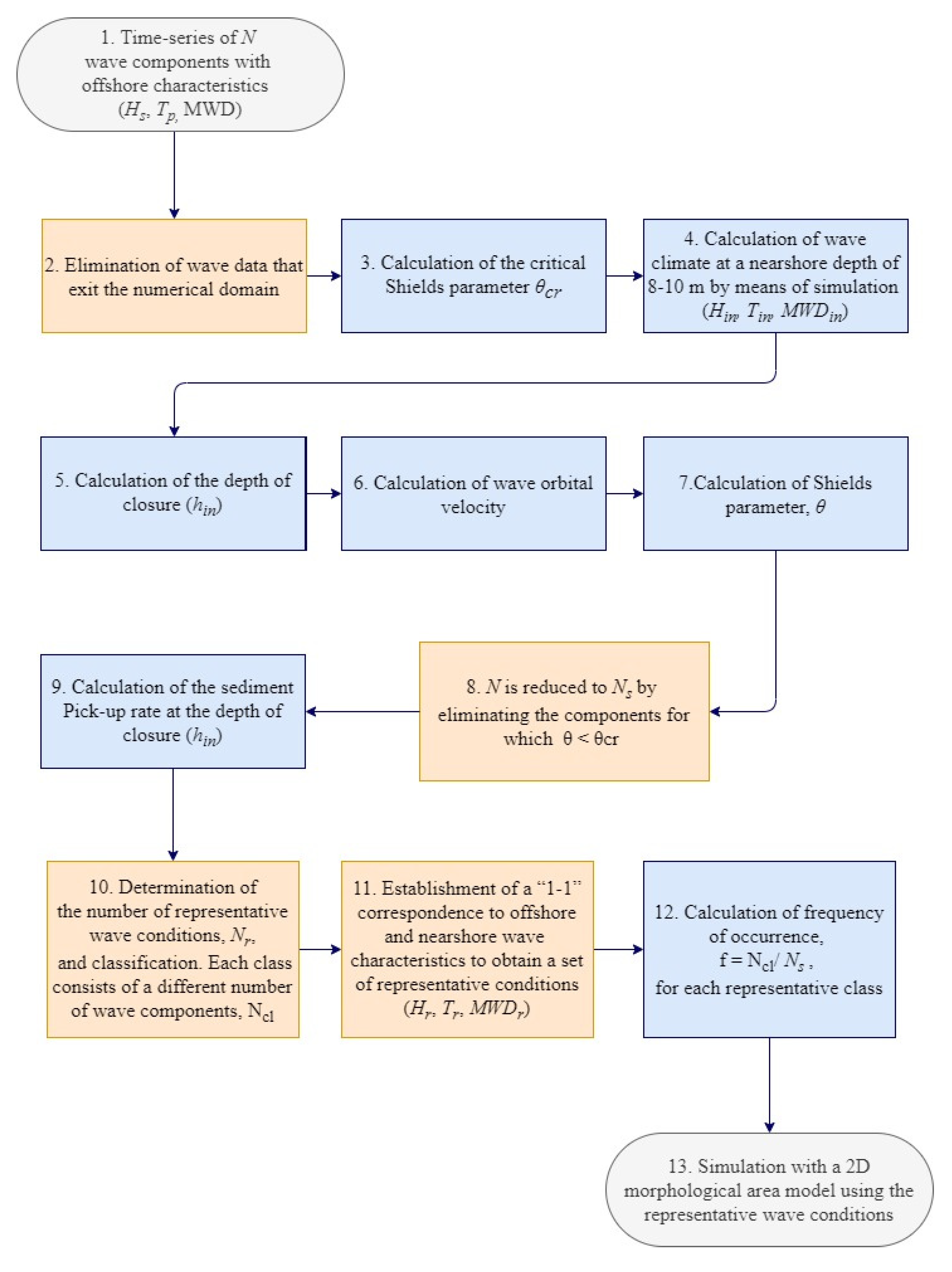
2.1.2. Layout of the Wave Schematization Method

In this subsection the distinct steps to determine the representative wave conditions, utilizing the pick-up rate input-reduction method are presented. The larger portion of this method is rather simple in conceptualization and execution and can be reproduced either by employing a simple computer code or a spreadsheet. The distinct steps of this method are as follows:

• Wave characteristic time-series (either by buoy measurements, or hindcast/forecast simulations) are obtained for a desirable time range T_tot on a single point offshore coinciding with the open boundary of the computational domain. The minimum wave characteristics that are required by the input-reduction method are H_s, T_p (or another characteristic wave period) and MWD (mean wave direction).
• The wave time-series are then filtered by disposing of wave data that do not contribute in shaping the bed evolution, namely wave components exiting the computational domain.
• Calculation of the critical Shields parameter θ_cr through Equation (1).
• Wave characteristics at a characteristic depth (at around h = 8–10 m, set as h = 8 m at the present study) are obtained. For this purpose, either a wave ray model (e.g., [29], a spectral wave model (e.g., [30,31,32], or a mild slope wave model [33,34] can be used. Here we use the parabolic mild slope model with non-linear dispersion characteristics MARIS-PMS. The reason for utilizing this model is the accuracy in prescribing the wave field in mildly sloping beaches due to incorporation of non-linearity and the saving of considerable computational time relatively to the time-dependent formulations of the aforementioned categories of models. After obtaining the wave climate in the nearshore area a “1-1” correspondence between each wave component offshore (H_s, T_p, MWD) and the wave characteristics at the characteristic depth (H_in, T_in, MWD_in), is established.
• Calculation of the depth of closure (h_in) for the particular time-series through the following equation, which is defined as the seaward limit of the littoral zone [35]:

  $${\mathrm{h}}_{\mathrm{in}}=8.9\overline{{\mathrm{H}}_{\mathrm{s}}}$$

  (12)

  where h_in [m] is the depth of closure and $\overline{{\mathrm{H}}_{\mathrm{s}}}$ [m] is the mean significant wave height at a characteristic depth h = 8–10 m, utilizing the wave characteristics calculated at step 4. The depth of closure was considered for the purpose of this research the critical depth after which no net sediment movement takes places. Consequently this depth will be later set for the calculation of the wave orbital velocity since the larger proportion of sediment transport takes place between h_in and the shoreline.
• Calculate the wave orbital velocity signal near the bed through Equation (3) for monochromatic or Equation (4) for spectral waves setting h = h_in.
• For each wave component (H_in, T_in, MWD_in) the friction factor f_w (Equation (9)), the bed shear stress due to waves τ_b,w (Equation (7)) and ultimately the Shields parameter θ (Equation (10)), are calculated
• If the θ < θ_cr the wave component is eliminated since it does not contribute in sediment motion. Through the “1-1” correspondence established at step 4, dispose the relative wave condition of the offshore time-series. The total number of wave components offshore N is thus reduced using the criterion of the initiation of motion at a total of N_s (with N_s ≤ N)
• Calculation of the sediment pick-up rate E_in through Equation (11) for each wave component at the depth of closure. Also the cumulative pick-up rate E for the aforementioned wave conditions is determined.
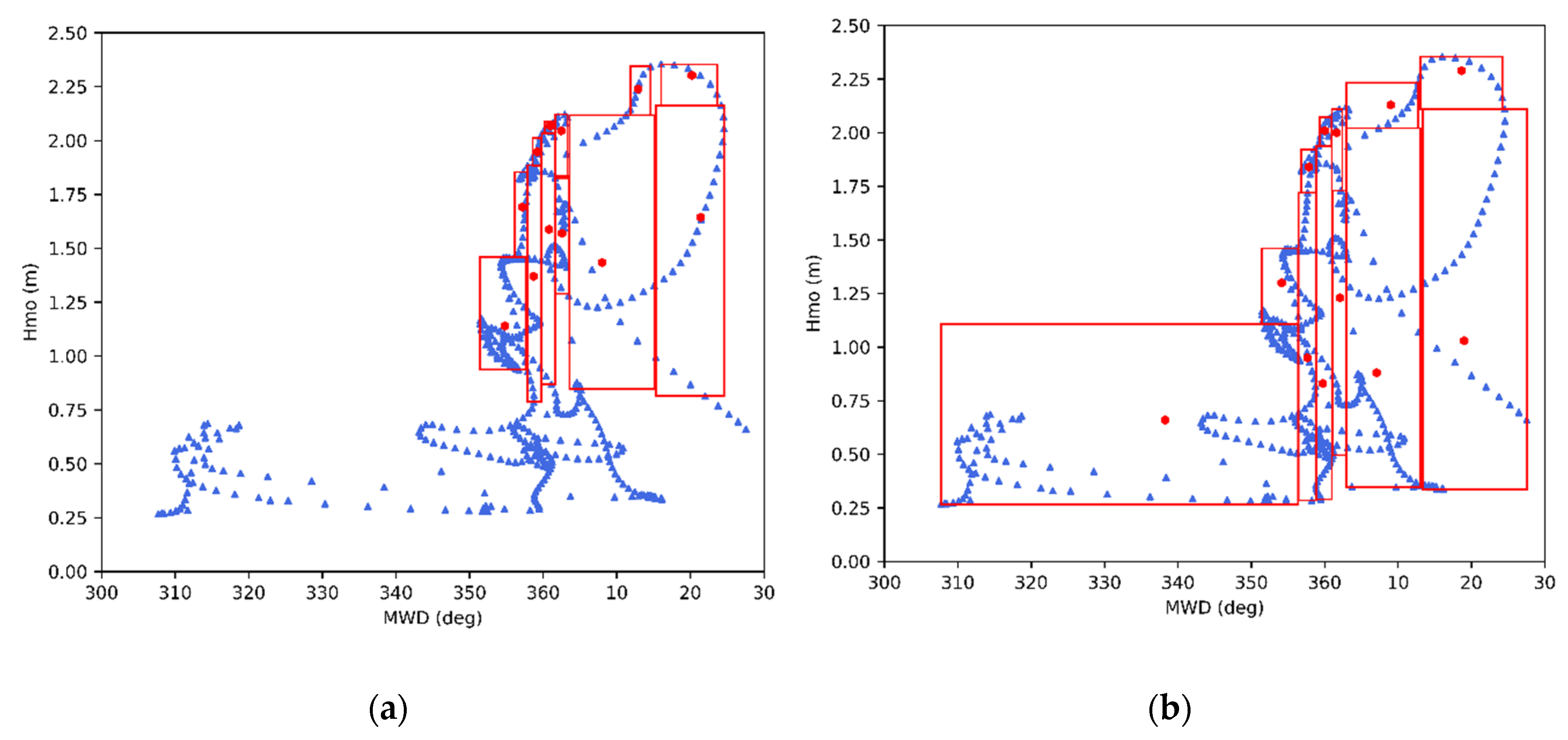
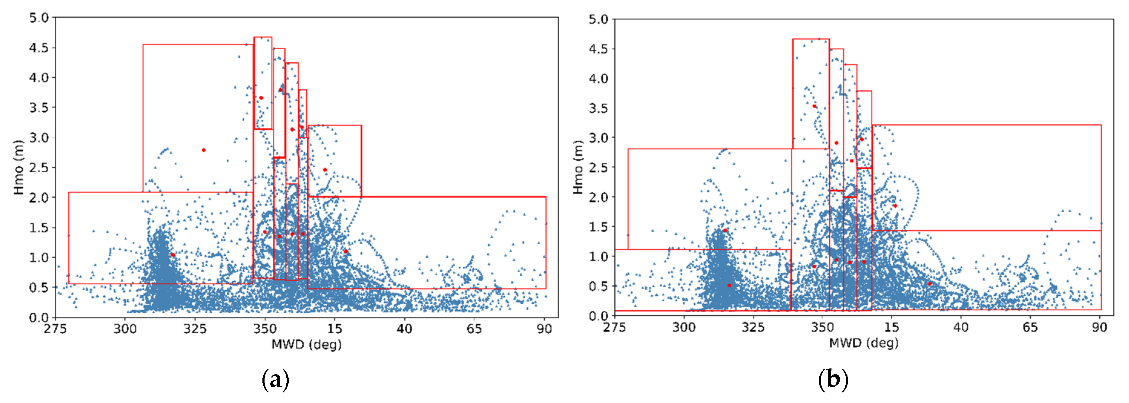
• The number of representative wave conditions N_r that will replace the full wave climate (e.g., 12 representative conditions) are determined. The number of representative conditions is based on discretion, however it is advised that a number between 6 and 30 conditions is chosen for sufficiently accurate model results regarding yearly wave climates [12]. Then, the wave components are divided in classes with respect to wave direction and wave height. The boundaries of each class in both direction and wave heights are determined the same wave as the energy-flux wave schematization method (see Section 2.2 for details). Each representative class is characterized by an equal fraction of the cumulative pick-up rate E (E/N_r) and can be described by a set of wave characteristics (H_r,in, T_r,in, MWD_r,in). Thus, it can be derived that each class consists of a different number of wave components, N_cl.
• Utilizing again the “1-1” correspondence of wave characteristics offshore and nearshore, we can obtain a set of representative conditions (H_r, T_r, MWD_r) in the offshore wave boundary by considering that the bounding limits of each representative class in the depth of closure coincide with the respective ones in deep water. A small numerical extrapolation error stems from the fact that each representative class in the offshore boundary might not be characterized by exactly equal fraction of sediment pick-up rate, since the pick-up rate was calculated for the corresponding wave conditions at shallower water. However, since the proposed input-reduction method concerns medium to long-term morphological bed changes, this error is considered to have a very small effect in shaping the ultimate bed evolution and thus can be neglected.
• The frequency of occurrence $\mathrm{f}=\frac{ {\mathrm{N}}_{\mathrm{cl}}}{\mathrm{Ns}}$ for each representative class is calculated, based on the wave components of each class relatively to the full set of conditions.
• Finally the simulation is executed with a 2D morphological area model using the representative wave conditions as forcing input. The total model run-time T_tot,r is a fraction of the full time series, denoted as ${\mathrm{T}}_{\mathrm{tot},\mathrm{r}}=\frac{{\mathrm{N}}_{\mathrm{r}}}{\mathrm{N}}{\mathrm{T}}_{\mathrm{tot}}$, since wave components unable to initiate sediment movement are eliminated in step 8 and have little to no contribution in shaping the bed evolution.

The flowchart of the wave schematization methodology based on the sediment pick-up rate is illustrated in Figure 1.

Through the use of this method one can obtain a set of representative conditions able to describe the morphological evolution of the bed in medium and long term, while also simultaneously reducing the simulation run-time. Thus, this method can be characterized as a bridge between input-reduction and model-reduction techniques, since it can lead in the considerable reduction of computation effort. It should be noted however that the total time that is saved is highly dependent on the wave climate that dominates the coast. For instance, in rather extreme offshore wave conditions where a large portion of waves contribute in initiation of sediment motion, the total number of disposable wave components can be rather small, leading in simulating a representative field for time equal to that of the full time-series. For morphological modelling of years to decades, however, one can assume that a rather large number of wave components will have little effect in the bed evolution, rendering the pick-up rate schematization method a valuable tool to coastal engineers and scientists.

2.2. The Energy Flux Wave Schematization Method (Benchmark Reduction Method)

The energy-flux wave schematization method is based on the concept of obtaining representative wave conditions which are separated at “equal energy intervals” [12,36]. For long-term morphological evolution simulations this concept is beneficial since the longshore sediment transport rates are proportional to the energy flux of the waves. The layout of the energy-flux input-reduction method is presented briefly below:

• Calculation of the wave energy flux $\left({\mathit{E}}_{\mathit{f}}\right)$ for each wave component of a time-series,

  $$E_f=\frac{1}{8}\rho g{H}_s^2{C}_g$$

  (13)

  where $\rho$ [kg/m³] is the water density, $H_s$ [m] is the significant wave height and $C_g$ [m/s] is the wave group celerity in deep water,
• Calculation of the total wave energy flux of the full wave time-series through:

  $$E_{tot}={{\displaystyle \sum }}^{}{E}_f$$

  (14)
• Division of the wave components in wave direction bins. For a predefined number of directional bins $(N_d)$ the time series are separated in bins, each consisting of an equal fraction of the total energy flux $(E_{tot}/N_d).$ Further division of the data in wave height bins. Separation is carried out for a predefined number of wave height bins $(N_h)$ with each bin characterized by an equal fraction of the total energy flux $(E_{tot}/(N_d·N_h).$
• A representative wave height for each bin is derived from the mean energy flux of the bin along with a mean energy-flux direction. The representative wave period is then defined as the mean period of the bin.

The energy-flux input-reduction method is easy to apply (calculations can usually be carried out within a spreadsheet) and as shown in [12] and [36], for long-term morphological bed evaluations in the order of years the obtained results are satisfactory. For the reasons stated above, the energy-flux method was used in the framework of this research as a “benchmark reduction method”, in order to assess how the newly developed pick-up rate schematization method fares not only in comparison to the bed evolution obtained through the full-time series, but also to the results obtained by a widely used wave schematization method.

2.3. Theoretical Background of Numerical Models

For the purpose of this research, a highly robust 2D composite model, namely MIKE21 Coupled Model FM [19] is utilized for the simulation of wave propagation, hydrodynamic circulation, sediment transport and morphology. In addition, for the calculation of nearshore wave characteristics at the depth of 8 m (see step 4, Figure 1) a mild-slope model of parabolic approximation, namely MARIS-PMS, is utilized in the present paper. A first noteworthy aspect of a parabolic approximation model is that it can be rapidly solved [34], which is essential for the pick-up rate input-reduction method in order to keep computational effort at a minimum when utilizing a large set of input wave conditions. Moreover, the specific model considers nonlinear amplitude dispersion effects and thus can produce significantly more accurate results than linear models. Nevertheless, it should be mentioned that parabolic approximation models are restricted to cases with negligible wave reflection and weak wave diffraction due to the lack of simulating back scattering. Therefore, the range of applicability is reduced for these models, rendering them suitable only for open coastal areas. In the following sections the governing equations and main features of the aforementioned numerical models are presented.

2.3.1. The MIKE21 Coupled Model FM Suite

For the long-term estimation of the bed evolution the process-based numerical model MIKE 21 Coupled Model FM [19] was used for the detailed description of hydrodynamics, waves, and sediment transport rates. The model has been used extensively in a variety of coastal engineering applications, with and without the presence of coastal protection structures (e.g., [1,13,37,38].

The MIKE21 Coupled model FM suite includes several complementary numerical models and tools three of which were used for the purpose of this research:

• MIKE21 SW, a 3rd generation spectral wave model based on the conservation of the wave action balance, suited for the propagation and transformation of waves in the coastal zone.
• MIKE21 HD, a depth-averaged hydrodynamic model based on the Reynolds-averaged Navier–Stokes equations of motion (RANS), for the description of the nearshore circulation.
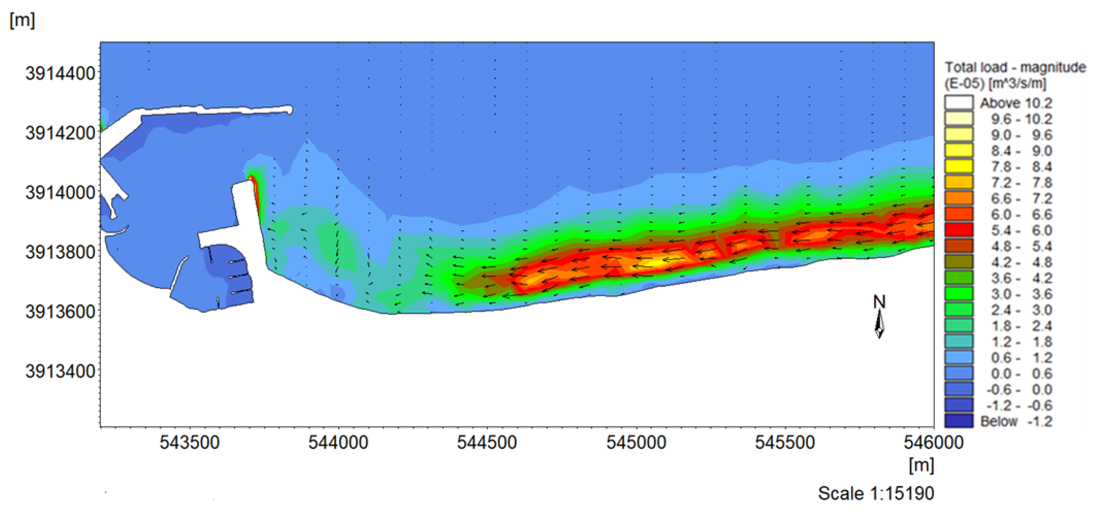
• MIKE21 ST, a sand transport and morphology updating model, used to calculate sediment transport rates and ultimately the morphological bed evolution.

The models are directly coupled, allowing for the interaction between waves and currents and the effect of bed level changes in waves and hydrodynamics. The calculations are performed in an unstructured finite element mesh, allowing for flexibility in calculations and a more precise representation of the coastline and complex topography features. The governing equations of each respective model will be presented briefly below. The MIKE 21 SW model [39] is a 3rd-generation spectral wave model suited for the propagation of waves in the oceanic scale and in nearshore areas. The governing equation of the model is based on the principle of conservation of the wave action-balance [40] which reads in Cartesian coordinates:

$$\frac{\partial \mathrm{N}}{\partial \mathrm{t}}{+\mathrm{c}}_{\mathrm{x}}\frac{\partial \mathrm{N}}{\partial \mathrm{x}}{+\mathrm{c}}_{\mathrm{y}}\frac{\partial \mathrm{N}}{\partial \mathrm{y}}{+\mathrm{c}}_{\mathsf{\sigma }}\frac{\partial \mathsf{{\rm N}}}{\partial \mathsf{\sigma }}{+\mathsf{\sigma }}_{\mathsf{\theta }}\frac{\partial \mathsf{{\rm N}}}{\partial \mathsf{\theta }}=\frac{\mathrm{S}}{\mathsf{\sigma }}$$

(15)

where $\mathrm{N}(\mathrm{x},\mathrm{y},\mathsf{\sigma },\mathsf{\theta },\mathrm{t})$ is the wave action density, ${\mathrm{c}}_{\mathrm{x}}$, ${\mathrm{c}}_{\mathrm{y}}$ are the propagation velocities in the spatial domain, ${\mathrm{c}}_{\mathsf{\sigma }}$ is the propagation velocity in the frequency domain and ${\mathrm{c}}_{\mathsf{\theta }}$ is the propagation velocity in the directional domain. All the aforementioned transfer velocities are computed according to the linear wave theory [40]. In the rhs of Equation (15), the term $\mathrm{S}$ denotes the source and sink terms of the energy balance equation (e.g., generation due to wind, white-capping dissipation, non-linear wave interactions, depth-induced breaking etc).

The hydrodynamic model MIKE21 HD [41] is based on the solution of the depth-integrated shallow water equations, expressed by the continuity and momentum equations in the Cartesian space:

$$\frac{\partial \mathrm{h}}{\partial \mathrm{t}}+\frac{\partial \mathrm{h}\overline{\mathrm{u}}}{\partial \mathrm{x}}+\frac{\partial \mathrm{h}\overline{\mathrm{v}}}{\partial \mathrm{y}}=\mathrm{h}\mathrm{S}$$

(16)

$$\begin{array}{l}\frac{\partial \mathrm{h}\overline{\mathrm{u}}}{\partial \mathrm{t}}+\frac{\partial \mathrm{h}{\overline{\mathrm{u}}}^2}{\partial \mathrm{x}}+\frac{\partial \mathrm{h}\overline{uv}}{\partial \mathrm{y}}=\mathrm{f}\overline{\mathrm{v}}\mathrm{h}-\mathrm{g}\mathrm{h}\frac{\partial \mathsf{\eta }}{\partial \mathrm{x}}-\frac{\mathrm{h}}{\mathsf{\rho }}\frac{\partial {\mathrm{p}}_{\mathrm{a}}}{\partial \mathrm{x}}-\frac{\mathrm{g}{\mathrm{h}}^2}{2\mathsf{\rho }}\frac{\partial \mathsf{\rho }}{\partial \mathrm{x}}+\frac{{\mathsf{\tau }}_{\mathrm{s}\mathrm{x}}}{\mathsf{\rho }}-\frac{{\mathsf{\tau }}_{\mathrm{b}\mathrm{x}}}{\mathsf{\rho }}-\\ \frac{1}{\mathsf{\rho }}(\frac{\partial {\mathrm{S}}_{\mathrm{x}\mathrm{x}}}{\partial \mathrm{x}}+\frac{\partial {\mathrm{S}}_{\mathrm{x}\mathrm{y}}}{\partial \mathrm{y}})+\frac{\partial }{\partial \mathrm{x}}\left(\mathrm{h}{\mathrm{T}}_{\mathrm{x}\mathrm{x}}\right)+\frac{\partial }{\partial \mathrm{y}}\left(\mathrm{h}{\mathrm{T}}_{\mathrm{x}\mathrm{y}}\right)+\mathrm{h}{\mathrm{u}}_{\mathrm{s}}{\mathrm{S}}_{\mathrm{x}}\end{array}$$

(17)

$$\begin{array}{l}\frac{\partial \mathrm{h}\overline{v}}{\partial \mathrm{t}}+\frac{\partial \mathrm{h}\overline{uv}}{\partial \mathrm{x}}+\frac{\partial \mathrm{h}{\overline{\mathrm{v}}}^2}{\partial \mathrm{y}}=\mathrm{f}\overline{u}\mathrm{h}-\mathrm{g}\mathrm{h}\frac{\partial \mathsf{\eta }}{\partial \mathrm{y}}-\frac{\mathrm{h}}{\mathsf{\rho }}\frac{\partial {\mathrm{p}}_{\mathrm{a}}}{\partial \mathrm{y}}-\frac{\mathrm{g}{\mathrm{h}}^2}{2\mathsf{\rho }}\frac{\partial \mathsf{\rho }}{\partial \mathrm{y}}+\frac{{\mathsf{\tau }}_{\mathrm{s}\mathrm{x}}}{\mathsf{\rho }}-\frac{{\mathsf{\tau }}_{\mathrm{b}\mathrm{x}}}{\mathsf{\rho }}-\\ \frac{1}{\mathsf{\rho }}(\frac{\partial {\mathrm{S}}_{\mathrm{x}\mathrm{y}}}{\partial \mathrm{x}}+\frac{\partial {\mathrm{S}}_{\mathrm{y}\mathrm{y}}}{\partial \mathrm{y}})+\frac{\partial }{\partial \mathrm{x}}\left(\mathrm{h}{\mathrm{T}}_{\mathrm{x}\mathrm{y}}\right)+\frac{\partial }{\partial \mathrm{y}}\left(\mathrm{h}{\mathrm{T}}_{\mathrm{y}\mathrm{y}}\right)+\mathrm{h}{\mathrm{v}}_{\mathrm{s}}{\mathrm{S}}_{\mathrm{x}\mathrm{x}}\end{array}$$

(18)

where $\mathrm{h}$ [m] is the total depth of the water column, $\overline{\mathrm{u}}$ and $\overline{\mathrm{v}}$ [m/s] are the depth-averaged velocity components in the x and y direction, respectively, $\mathsf{\eta }$ [m] is the surface elevation, $\mathrm{f}$ [-] is the Coriolis parameter, $\mathsf{\rho }$ [kg/m³] is the water density, ${\mathrm{S}}_{\mathrm{xx}}$, ${\mathrm{S}}_{\mathrm{yy}}$, ${\mathrm{S}}_{\mathrm{xy}}$, are components of the radiation stress tensor, ${\mathrm{p}}_{\mathrm{a}}$ [N/m²] is the atmospheric pressure, $\mathrm{S}$ [m³/s] being the magnitude of point sources, with ${\mathrm{u}}_{\mathrm{s}}$, ${\mathrm{v}}_{\mathrm{s}}$. [m/s] being the velocity vectors of the point discharge and ${\mathrm{T}}_{\mathrm{xx}}$, ${\mathrm{T}}_{\mathrm{yy}}$, ${\mathrm{T}}_{\mathrm{xy}}$ [N/m²] denoting lateral stresses including viscous, turbulent friction and differential advection.

The MIKE 21 ST model [42] calculates the sediment transport rates and the morphological bed evolution either in a pure current case, or under the combined effect of waves and currents.

For the case of wave and current induced sediment transport, the rates are calculated by linear interpolation on an externally formed sediment transport table. The core of this utility is a quasi-three-dimensional sediment transport model (STPQ3D). The model calculates the instantaneous and time-averaged hydrodynamics and sediment transport in the two horizontal directions.

The determination of the bed level evolution is the rate of bed level change $\frac{\partial \mathrm{z}}{\partial \mathrm{t}}$ at the element cell centers. This parameter is obtained by solving the well-known equation of sediment continuity, denoted as the Exner equation:

$$\frac{\partial \mathrm{z}}{\partial \mathrm{t}}=-\frac{1}{(1-\mathrm{n})}\left(\frac{\partial {\mathrm{S}}_{\mathrm{x}}}{\partial \mathrm{x}}+\frac{\partial {\mathrm{S}}_{\mathrm{y}}}{\partial \mathrm{x}}-\mathsf{\Delta }\mathrm{S}\right)$$

(19)

where n [-] is the sediment porosity, ${\mathrm{S}}_{\mathrm{x}}$, ${\mathrm{S}}_{\mathrm{y}}$ [m²/s] is the total load sediment transport rates in the x and y direction respectively and $\mathsf{\Delta }\mathrm{S}$ [m/s] is a sediment source or sink term. The new bed level is then obtained by a forward in time differential scheme.

2.3.2. The MARIS-PMS Wave Model

In order to calculate the nearshore wave characteristics a Parabolic Mild Slope model is implemented, utilizing its accuracy in prescribing the wave field in mildly sloping beaches and the saving of considerable computational time. In particular, the wave model MARIS-PMS [34] presented herein is based on the work of [43] who derived a parabolic equation, in the form of a cubic Schrödinger differential equation, governing the complex amplitude, A, of the fundamental frequency component of a Stokes wave. Darlymple et al. [44] improved the parabolic equation and its range of validity by developing approximations based on minimax principles in order to allow for large-angle propagation and rendering the approximation suitable for large scale applications, thus proposing the following governing equation:

$${\mathrm{C}}_{\mathrm{g}}{\mathrm{A}}_{\mathrm{x}}+\mathrm{i}(\overline{\mathrm{k}}-{\mathrm{a}}_0\mathrm{k}){\mathrm{C}}_{\mathrm{g}}\mathrm{A}+\frac{1}{2}{\left({\mathrm{C}}_{\mathrm{g}}\right)}_{\mathrm{x}}\mathrm{A}+\frac{\mathrm{i}}{\mathsf{\omega }}({\mathsf{\alpha }}_1-{\mathrm{b}}_1\frac{\overline{\mathrm{k}}}{\mathrm{k}}){\left(\mathrm{C}{\mathrm{C}}_{\mathrm{g}}{\mathrm{A}}_{\mathrm{y}}\right)}_{\mathrm{y}}-\frac{{\mathrm{b}}_1}{\mathsf{\omega }\mathrm{k}}{\left({\mathrm{C}\mathrm{C}}_{\mathrm{g}}{\mathrm{A}}_{\mathrm{y}}\right)}_{\mathrm{y}\mathrm{x}}+\frac{{\mathrm{b}}_1}{\mathsf{\omega }}(\frac{{\mathrm{k}}_{\mathrm{x}}}{{\mathrm{k}}^2}+\frac{{\left({\mathrm{C}}_{\mathrm{g}}\right)}_{\mathrm{x}}}{2\mathrm{k}{\mathrm{C}}_{\mathrm{g}}}){\left({\mathrm{C}\mathrm{C}}_{\mathrm{g}}{\mathrm{A}}_{\mathrm{y}}\right)}_{\mathrm{y}}+\frac{\mathrm{i}\mathsf{\omega }{\mathrm{k}}^2}{2}\mathrm{D}|\mathrm{A}{|}^2\mathrm{A}+\frac{\mathrm{w}}{2}\mathrm{A}=0$$

(20)

where the parameter $\mathrm{D}$ is given by $\mathrm{D}=\frac{\left({\cos \mathrm{h}4\mathrm{kh}+8-2\tan \mathrm{h}}^2\mathrm{kh}\right)}{{8\sin \mathrm{h}}^4\mathrm{kh}}$, the complex amplitude $\mathrm{A}$ is related to the water surface displacement by ${\mathsf{\eta }=\mathrm{Ae}}^{-\mathrm{i}\left(\mathrm{kx}-\mathsf{\omega }\mathrm{t}\right)}$, $\mathrm{k}$ the local wave number related to the angular frequency of the waves, $\mathsf{\omega }$ [rad/s], and the water depth, $\mathrm{h}$ [m]. $\overline{\mathrm{k}}$ [rad/m] is a reference wave number taken as the average wave number along the y-axis, $\mathrm{C}$ [m/s] is the phase celerity, ${\mathrm{C}}_{\mathrm{g}}$ [m/s] is the group celerity and $\mathrm{w}$ is a dissipation factor. Finally$,\mathrm{coefficients}$ ${\mathrm{a}}_0$, ${\mathsf{\alpha }}_1$ and ${\mathrm{b}}_1$ depend on the aperture width chosen to specify the minimax approximation [45]. The combination of ${\mathrm{a}}_0=0.994733$, ${\mathsf{\alpha }}_1=-0.890065$, and ${\mathrm{b}}_1=-0.451641$ was found in [45] to give reasonable results for a maximum angular range of 70° and is applied in the MARIS-PMS model.

MARIS-PMS takes into account energy dissipation due to bathymetric breaking following the formulation of [46], and bottom friction, which is modelled through the formulation of [47].

MARIS-PMS incorporates non-linear dispersion characteristics, in order to improve model results in the nearshore area, which can be obtained by introducing an approximate non-linear amplitude dispersion relationship, such as that presented in [48].

Instead of utilizing a unique mathematical expression over the entire numerical domain, combined models can be applied (e.g., [49,50] in order to incorporate high nonlinearity at any depth. Utilizing this approach, the wave celerity is assumed to vary spatially within the simulation, and the nonlinear dispersion relation to be applied is subject to the local Ursell number $\mathrm{Ur}={\mathrm{HL}}^2/{\mathrm{h}}^3$ and wave steepness $\mathrm{s}=\mathrm{H}/\mathrm{L}$, in relation to the valid regions of analytical wave theories.

Therefore, for $\mathrm{s}>0$ and $\mathrm{Ur}>4000$ and $\mathrm{H}/\mathrm{h}<0.78$ a modified cnoidal equation is adopted:

$${\mathsf{\omega }}^2{=\mathrm{gk}}^2\mathrm{h}\left(1+\mathrm{f}\left(\mathrm{m}\right)\mathrm{H}/\mathrm{h}\right)$$

(21)

where $\mathrm{f}\left(\mathrm{m}\right)$ a function of the parameter $\mathrm{m}$, the modulus of the elliptic functions. Bell et al. [51] assumed a constant value $\mathrm{f}\left(\mathrm{m}\right)=0.4$ which is adopted in the model formulation.

Conversely, for$\mathrm{s}>0$ and $\mathrm{Ur}>4000$ and $\mathrm{H}/\mathrm{h}>0.78$ the solitary wave dispersion relation is used:

$${\mathsf{\omega }}^2{=\mathrm{gk}}^2\mathrm{h}(1+\mathrm{H}/\mathrm{h})$$

(22)

In the surf zone, the aforementioned solitary wave relation behaves similarly with the simple approach to model wave celerity through a modified shallow water approximation [52]:

$${\mathsf{\omega }}^2{=\mathrm{a}}^2{\mathrm{gk}}^2\mathrm{h}$$

(23)

where a typical value of the coefficient $\mathrm{a}$ is set to 1.3.

In order to tackle numerical discontinuities at the coupling boundaries, due to variation across Stokes, cnoidal and solitary divisions, a weighted moving average (WMA) technique is incorporated to smooth the values of celerity in the transition windows from one theory to another [34]. The analytical method was utilized in the present study to calculate significant wave heights, periods and directions, at a characteristic depth of 8 m (see step 4 of Section 2.1.2.). It is considered that this method can achieve a fine compromise between robust and time-efficient calculations while attaining non-linear dispersion characteristics in the shallow water area. Besides, for the calculation of wave characteristics and the subsequent calculation of the depth of closure, [53] proposed the use of linear wave models. We consider the use of a parabolic mild slope wave model for this purpose to be an improvement on the methodology improving the accuracy of the estimation of wave heights in the nearshore, while simultaneously keeping simulation times at reasonable levels [34].

3. Method Implementation

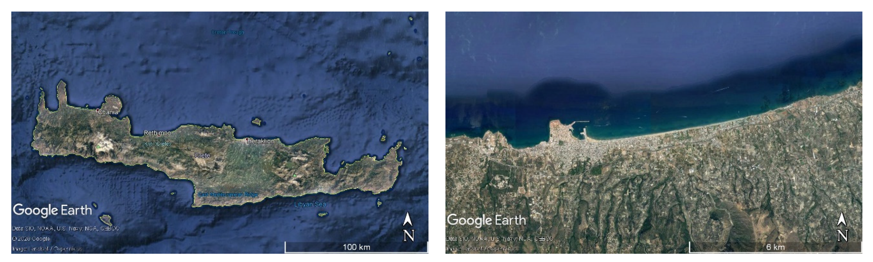
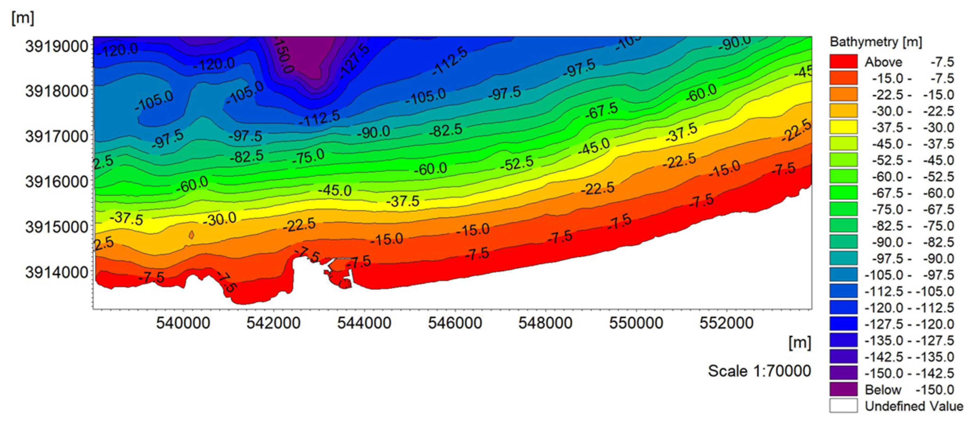
3.1. Study Area

The input-reduction method based on the sediment pick-up rate was implemented using the MIKE21 Coupled Model FM suite in the coast located in the close vicinity of the port of Rethymno, in the island of Crete, Greece. The area of interest, shown in Figure 2, includes the aforementioned port, located in the northern end of Crete within the homonymous bay and the adjacent coastal area at the east and a coastline of approximately 4 km in length. The aforementioned coastline comprises mostly fine sand, with a median sediment diameter of $d_{50}=0.15\mathrm{mm}$, which was used for the morphological simulations. Being a highly urbanized area, commercial, administrative, cultural and tourist activities are concentrated along the north coast where the city is located. Consequently, a medium to long-term prediction of the bed evolution and ultimately the displacement of the shoreline, is of particular interest to engineers/scientists and the public.

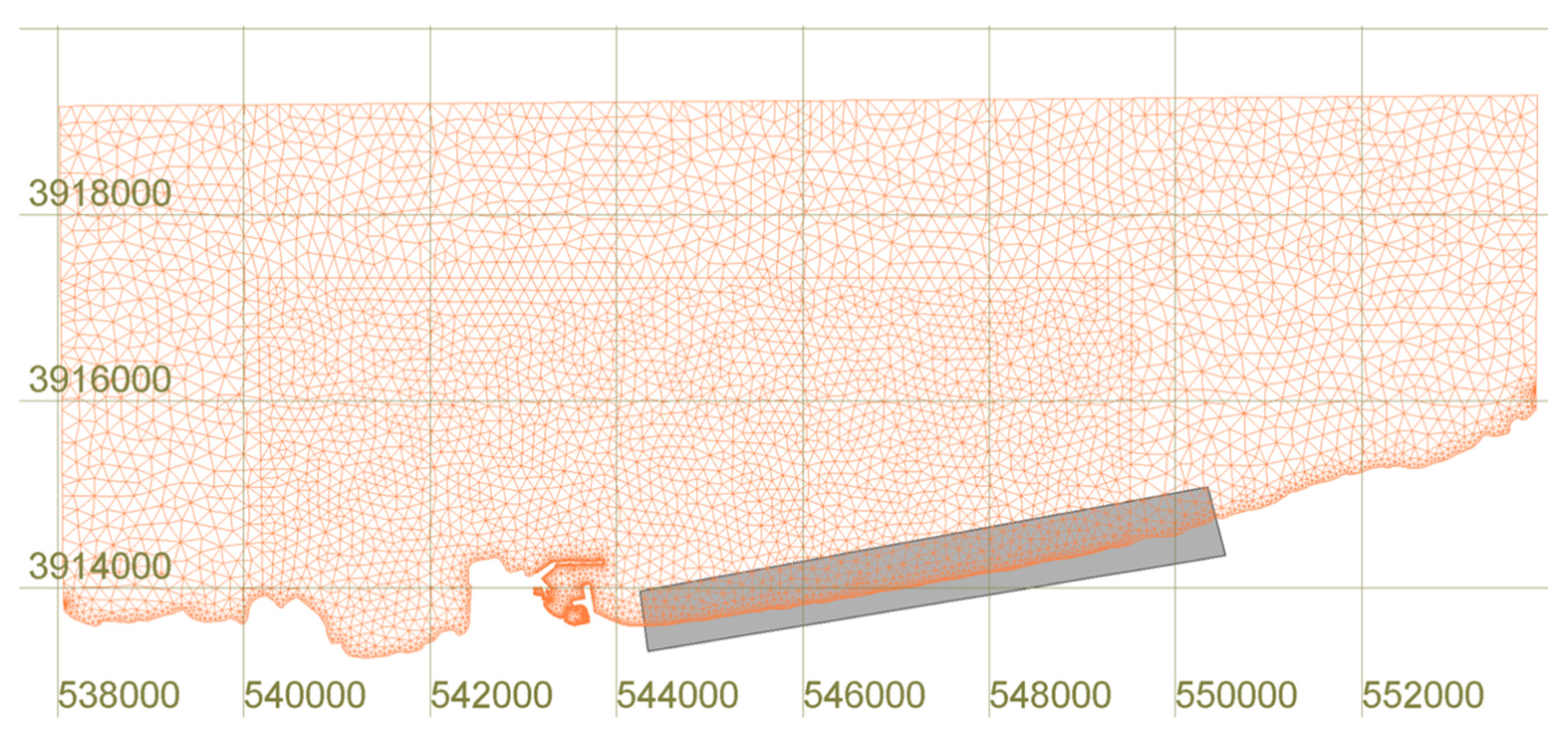
3.2. Mesh Generation

In order to simulate the morphological bed evolution of the Rethymno coast, an unstructured finite element mesh was constructed. Three mesh density levels were used for the discretization of the domain, with the coarser area being near the offshore and the lateral wave boundaries, and the denser one covering an extend of 3.5 km long and 10.0 km wide. A third density level was established extending at about 250 m offshore the western coastline. For the solid boundaries, a vertice-adaptive mesh generation scheme allowed the construction of relatively small finite elements in the solid boundaries, allowing for the more detailed description of the bathymetric variations in shallow water areas. Regarding the dimensions of the interior triangular elements, they are comprised of a mean nominal length of about 100 m, with the largest element size being 293 m and the minimum 0.71 m. The bathymetry was digitized using QGIS software [55], utilizing nautical maps from the Navionics web application [56] as input. The final bathymetric mesh for the study area is presented in Figure 3.

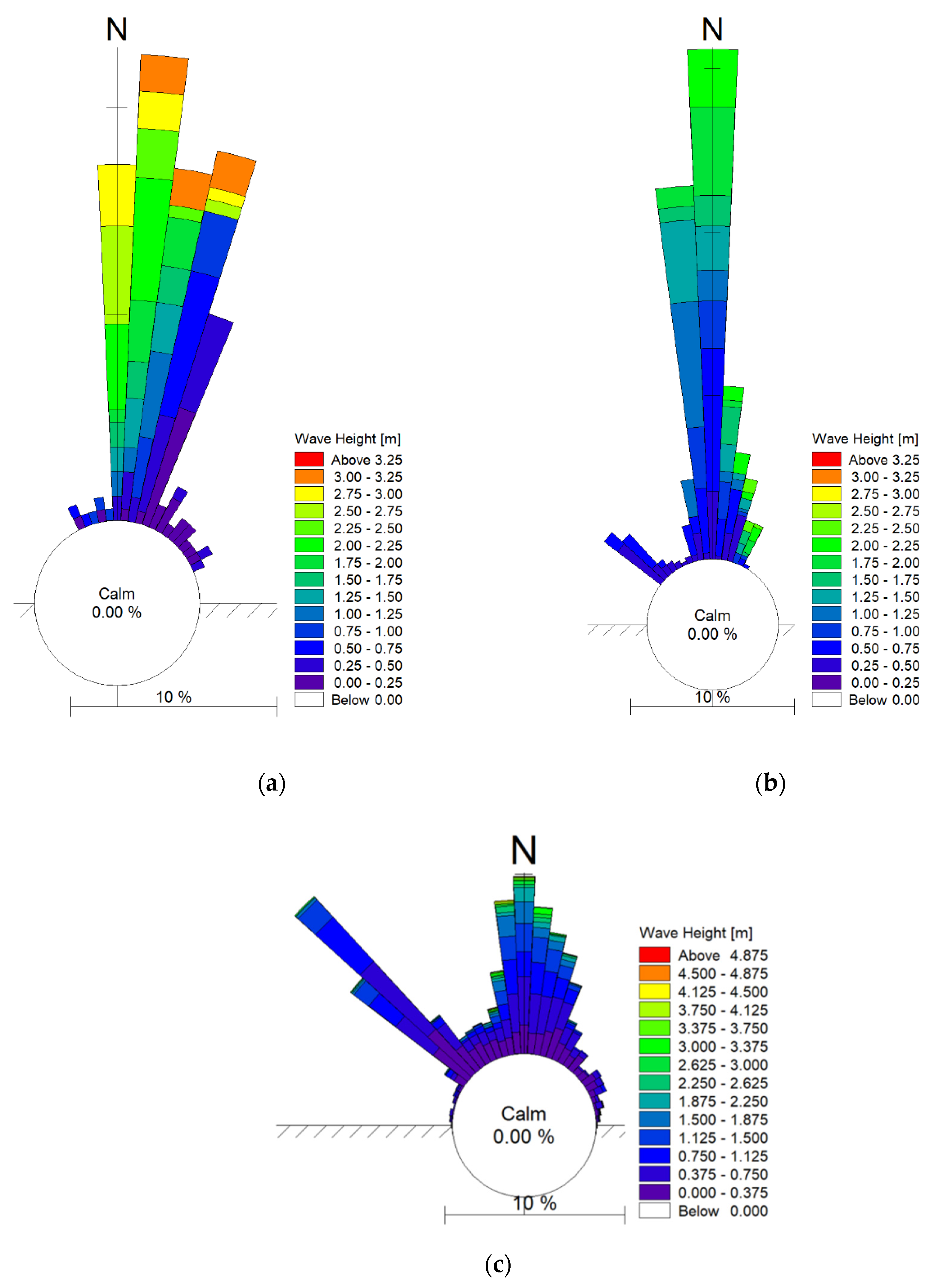
3.3. Offshore Wave Data

To force the 3rd generation spectral wave model MIKE21 SW time series of wave characteristics were obtained at the north boundary of the computational mesh, namely spectral wave height, peak wave period and mean wave direction from CMEMS [8] database for a time range covering 02/2012–02/2017. For this purpose, the regional package MEDSEA_HINDCAST_WAV_006_012 [57], a multi-year wave hindcast product composed of hourly wave parameters at 1/24° horizontal grid resolution was utilized. The dataset is produced by the corresponding Mediterranean Sea Forecast package which in turn is a wave model based on the well-established spectral wave model WAM Cycle 4.5.4 [58]. The extracted offshore time series were also fed to the MARIS-PMS model, in order to obtain wave characteristics at the depth of 8 m seaward the sandy coastline near the Rethymno port, to be used in the calculations of the depth of closure. The input-reduction method was implemented for three distinct scenarios, firstly a wave time series at hourly intervals for 7 days, from 19/12/2012 to 26/12/2012, secondly a wave time series for 20 days from 17/08/2012 to 06/09/2012, and lastly for a time series covering a full year (365 days) of wave records, from 01/01/2012 to 01/01/2013. A Morfac of 1, 20 and 100 was used for the three separate cases respectively, in order to validate the input-reduction method without and with the effect of the morphological acceleration factor and assess its effect on the method’s sensitivity. For each case, 3 set of simulations were performed, namely:

• A simulation consisting of the full time series at the offshore boundary, hereafter denoted as Reference simulation
• A simulation using 12 representatives as forcing parameters calculated with the pick-up rate method, hereafter called pick-up rate simulation
• A simulation using 12 representatives calculated with the energy-flux input-reduction method, hereafter denoted as energy-flux simulation, to assess how the pick-up rate method fares against a well-established wave schematization technique.

The time series, especially that covering the extent of 7 days, was desirable to contain wave height conditions with significant variation, in order to assess the performance of the pick-up rate simulation in a rather diverse wave climate. The rose plot of wave heights for the time series comprising 7 and 20 days are shown in Figure 4. It can be observed that low, mild and moderate wave conditions, in terms of wave height, are present in both datasets. Nevertheless, certain differences can be observed regarding the distribution of wave heights, since the dataset of 7 days is consisted of more extreme wave conditions (maximum wave height H_mo = 3.2 m) while the dataset of 20 days was characterized by milder wave conditions with a maximum wave height H_mo = 2.35 m. Regarding the dataset covering the extend of the year, the wave climate was more diverse, with a minimum wave height of 0.09 m and a maximum wave height of 4.66 m. From the initial filtration of the waves that exit the computational domain and therefore have no effect on the morphological bed evolution, the dataset was reduced from 8762 hourly changing wave records to 8219. The vast majority (over 70 %) of the incident waves are entering the computational domain from the north sector, as shown in Figure 4.

3.4. Obtained Representative Wave Conditions

A total of 12 conditions were chosen to represent the input wave data for all datasets according to [12], who considered them to be adequate to accurately describe the morphological bed evolution induced by yearly wave climates. Thus, we consider 12 conditions to be able to represent satisfactorily the wave climate of the smaller datasets that were used for the purpose of this research, as well as the dataset covering a full year. In

Table 1. Representative wave conditions from the time series of 7 days, using the pick-up rate and the energy-flux wave schematization methods.

Class	Pick-up Rate Method Representatives				Energy Flux Method Representatives
	Hmo (m)	Tp (s)	MWD (°)	Frequency (%)	Hmo (m)	Tp (s)	MWD (°)	Frequency (%)
1st	1.78	6.96	1.30	14.94	1.23	5.87	357.57	10.84
2nd	2.77	8.20	1.65	4.60	2.55	8.09	1.46	3.01
3rd	2.51	7.63	2.35	5.75	2.53	7.63	2.31	3.61
4th	2.77	8.01	2.01	4.60	2.78	8.01	1.93	2.41
5th	2.30	7.53	3.27	8.05	1.96	7.09	3.69	6.02
6th	2.94	8.39	3.24	3.45	2.76	8.09	2.99	3.01
7th	1.74	6.99	4.85	19.54	1.44	6.38	5.14	10.24
8th	2.65	8.01	4.73	4.60	2.88	8.20	5.35	2.41
9th	1.70	7.12	8.47	18.39	1.44	6.69	8.86	10.24
10th	3.19	8.39	8.50	2.30	2.90	8.01	8.62	2.41
11th	1.88	6.89	12.78	10.34	0.52	4.77	21.63	43.37
12th	3.16	7.63	12.49	3.45	3.08	7.63	14.37	2.44

the representative wave conditions (defined by the spectral wave height ${\mathrm{H}}_{\mathrm{mo}}$, peak wave period ${\mathrm{T}}_{\mathrm{p}}$, mean wave direction $\mathrm{MWD}$ and frequency of occurrence) obtained by implementing the pick-up rate method, along with those stemming from the energy-flux method are presented for the dataset of 7 days.

It can be observed that both methods for the larger part have similar directional bins expressed by the representative values, although the pick-up rate method possesses larger wave heights with a higher frequency of occurrence for these particular classes. This can be attributed to the elimination of wave heights that are unable to initiate sediment motion, which results in the translocation of the center of the wave height bins in higher values, when compared to the energy-flux method. Furthermore, in Figure 5, the total dataset of 20 days along with the representative conditions is presented in a scatter plot, for both the pick-up rate and the energy-flux method. It can be observed for the particular case that the directional bins are quite different when comparing the two methods, due to the low-energy wave conditions generated from a direction of 300°–350° which are not capable of initiating sand motion and consequently are not taken into consideration by the pick-up rate method.

The obtained representatives calculated through the pick-up rate and the energy-flux input-reduction methods for the dataset covering the extent of a year are presented as a scatter plot in Figure 6. Once again it is evident that due to the elimination of low energy wave conditions the representatives obtained through the implementation of the pick-up rate method have larger wave heights compared to the ones stemming from the energy-flux method while the frequency of occurrence is more or less the same. An increase in both representative wave height and frequency of occurrence for the pick-up rate signifies that the specific classes contains a large amount of wave components that are able to initiate sediment motion. Effectively by introducing the Shield’s criterion of incipient motion one can obtain representative wave conditions that correspond to the more energetic wave condition of the wave climate while increasing their impact in the prediction of the morphological bed evolution.

4. Results and Discussion

In the following section, the results that were obtained by implementing the pick-up rate method by applying the process-based model MIKE21 Coupled Model FM are presented. In order to evaluate the performance of 2D morphological area models we calculate various statistical parameters which are described in detail in [59]. The performance of a morphological model can ultimately be assessed by calculating its bias, accuracy and skill. The most commonly used measure of the latter quantity is the Brier Skill Score (BSS) which has been applied in a plethora of morphological modelling applications (i.e., [15,60,61]. It is calculated through the following relationship:

$$\mathrm{BSS}=1-\frac{\mathrm{MSE}\left(\mathrm{Y},\mathrm{X}\right)}{\mathrm{MSE}\left(\mathrm{B},\mathrm{X}\right)}=1-\frac{{\langle \left(\mathrm{Y}-\mathrm{X}\right)}^2\rangle }{{\langle \left(\mathrm{B}-\mathrm{X}\right)}^2\rangle }$$

(24)

where Y denotes the predicted (modelled) quantity, X denotes a measured quantity, corresponding to the reference simulation for the present study due to lack of measurements, and B is a baseline prediction, usually referring to the initial bathymetry, assuming no alteration of the bed. Additionally, the square brackets denote average quantities over the whole domain. In

Table 2. Classification table for the Brier Skill Score (BSS) as proposed by [59]. (Adapted from [59], with permission from Elsevier, 2004).

	BSS
Excellent	1.0–0.5
Good	0.5–0.2
Reasonable/fair	0.2–0.1
Poor	0.1–0.0
Bad	<0.0

the classification scores for the BSS according to [59] in order to estimate the performance of a given morphological evolution model are shown:

We evaluate the performance of the morphological model in an area extending about 450 m offshore (at a maximum depth of about 9 m) the eastern coastline adjusted to the port. We chose to focus on this area (enclosed by the polygon shown in Figure 7), since it consists mostly of a sandy uniform bed and is of high interest to the public due to various tourist activities concentrated there. We also avoid evaluating the performance of the process-based model in the close vicinity of the port of Rethymno, since the phase-averaged approach utilized by the spectral wave driver MIKE21 SW is not suited to deal with inhomogeneities and coherent interfaces present in the wave field due to reflection and diffraction [62,63].

The estimation of wave heights in the characteristic depth of 8.0 m to subsequently calculate the depth of closure was carried out using the MARIS-PMS wave model for the full datasets of 7 and 20 and 365 days, with the computed depth of closure being 8.67 m, 6.95 m and 6.69 for each dataset respectively. No wave breaking took place as expected, however minor changes in the wave height were observed due to the energy bunching effect attributed mostly to shoaling and secondly to wave refraction.

4.1. Morphological Bed Evolution for the Dataset of Seven Days

In the present section the morphological bed evolution of the area of interest using the forcing dataset of 7 days is presented and discussed. The most dominant wave direction turned out to be the northern, as shown by the representative wave conditions in Table 1. Consequently, the prevailing hydrodynamic and sediment transport vector component’s direction for the area of interest was directed from east to the west, as shown in Figure 8, resulting mostly in accretive patterns in the beach face.

From the total of 168 initial hourly changing wave heights 88 of them lead to initiation of sediment motion by implementing the Shields criterion as was discussed in Section 2.1. Therefore the full dataset was reduced by a percentage of 47.62%, using the pick-up rate input-reduction method presented in this paper. Regarding model run-times, the Reference simulation corresponding to the induced morphological evolution of the complete dataset, resulted in a run-time of 133.3 h. Conversely, the reduced dataset obtained from the implementation of the pick-up rate method achieved a run-time of 79.19 h. Thus, a reduction of model run-time by 59.42% was achieved by implementing a Morfac value of 1 (no acceleration for this simulation). For reference, the energy-flux simulation was completed after a run-time of 131.2 h. The relatively small effective run-time reduction achieved through this method can attributed to the preprocessing of data (small number of wave components compared to the full dataset) and not so much to the computational process. By utilizing a Morfac of 1, the reduction of model run-time can essentially be attributed to the newly developed input-reduction method. This particular feature is considered to be a valuable asset for engineers and scientists wanting to perform medium to long-term morphological simulations while simultaneously reducing the additional numerical burden.

Regarding the model performance, for the area enclosed within the polygon shown in Figure 7, nodal values of the bed level inside the particular domain were extracted both for the Reference simulation and the pick-up rate simulation. Additionally the corresponding nodal values for the simulation utilizing the energy-flux input-reduction method were extracted to compare how it fares against the newly developed method based on the sediment pick-up rate. The model performance was assessed by calculating measures of bias and accuracy, namely the mean absolute error (MAE), mean square error (MSE) and root mean square error (RMSE). Lastly we focused on the skill evaluation of the model by calculating the BSS and categorizing the simulation as shown in Table 2. The measures obtained for the area of interest are shown in

Table 3. Statistical parameters obtained in the area of interest for both the pick-up rate simulation and the energy-flux simulation-Dataset of 7 days.

	Pick-Up Rate Method	Energy Flux Method
Bias	−0.0054	−0.0101
MAE(Y,X)	0.0218	0.0233
MSE(Y,X)	0.0018	0.0020
RMSE(Y,X)	0.0429	0.0450
BSS	0.9300	0.9200

(please see Supplementary Materials for the detailed calculations of the statistical measures).

From the above it can be derived that both the pick-up rate method and the energy-flux method can be categorized as excellent in regards to the BSS. As far as the model bias is concerned, the numerical model slightly underpredicts the morphological changes, albeit for a few mm. All accuracy measures are deemed acceptable for short-term morphological simulations. It should be stated that the pick-up rate method fares slightly better than the energy-flux method for this particular dataset. This can be attributed to the fact that for relatively small datasets of input data, the higher complexity of the pick-up rate method and subsequent calculations can offer slightly more detailed prediction of the morphological bed evolution. However, on the other hand the pick-up rate method is highly dependent on the formulations used for the calculation of physical quantities, such as the friction factor due to waves and wave orbital velocity and consequently more testing to verify the previous statement should be carried out.

4.2. Morphological Bed Evolution for the Dataset of 20 Days

For the particular dataset, the hydrodynamic and sediment transport patterns were relatively the same as the results shown in the previous section. This can be attributed to the prevailing waves propagating from the northern sector which again dominate the wave climate, as shown in Figure 4. For all the simulation scenarios of this section we applied a value of Morfac = 20 in order to ultimately assess how the pick-up rate method fares in longer datasets when used in tandem with a model-reduction technique.

From the total of 481 initial hourly changing wave heights, 216 of them in deep water satisfy the Shields criterion of incipient motion. Therefore the full dataset was reduced by a percentage of 45.53%, for the purpose of implementing the pick-up rate method. Regarding model run-times, the Reference simulation corresponding to the induced morphological evolution of the complete dataset, resulted in a run-time of 24.47 h, whereas the energy-flux simulation achieved a model run-time of 23.21 h. Conversely, the reduced dataset resulting from the implementation of the pick-up rate method achieved a run-time of 12.57 h, leading to a reduction of 51.37% of total model run-time. This is a significant portion of model reduction when taking into account the further run time reduction achieved through the use of Morfac.

Utilizing the same procedure as §4.1 bed level values were extracted for the resulting model predictions (through the implementation of pick-up rate and energy-flux methods) and the “measured” values obtained through the reference simulation. The obtained bias, accuracy and skill measures for the area of interest illustrated in Figure 7 are shown in

Table 4. Obtained statistical parameters in the area of interest for both the pick-up rate simulation and the energy-flux simulation dataset of 20 days.

	Pick-Up Rate Method	Energy Flux Method
Bias	−0.0177	−0.0058
MAE(Y,X)	0.0633	0.0535
MSE(Y,X)	0.0096	0.0066
RMSE(Y,X)	0.0980	0.0813
BSS	0.8300	0.8800

, while the detailed calculations of the statistical quantities for the particular dataset are presented in the Supplementary Materials.

It can be observed that the situation for the longer dataset of 20 days comparing the scores of the two simulations are reversed, as the energy-flux method performs better in all assessing categories. The slightly worse performance of the pick-up rate input-reduction method can be attributed to the elimination of the low-energy wave conditions. It should be stated though that both simulations achieve a score of “Excellent” once again, validating the ability of both methods to predict the morphological bed evolution for this particular set of input conditions. Thus, it is considered that for medium term morphological modelling applications, a small decrease in accuracy is insignificant compared to the model run-time reduction achieved through implementation of the pick-up rate method.

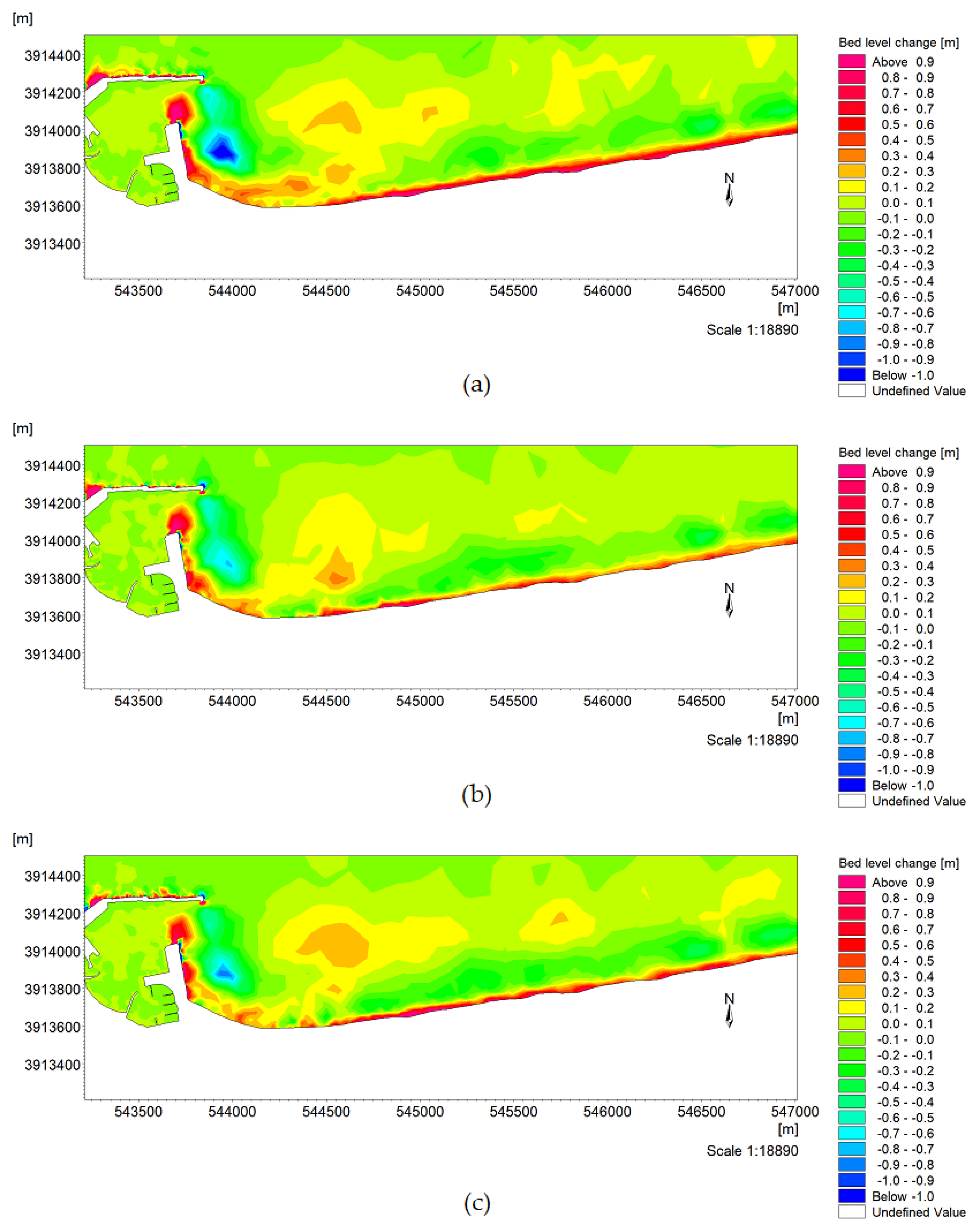
4.3. Morphological Bed Evolution for the Dataset of a Year

In the present section, the predicted bed level changes obtained through the pick-up rate and the energy-flux simulation are compared with the Reference simulation for the dataset covering a full year of wave data. This comparison is of significant importance, since it can provide the basis for the assessment of the performance of the pick-up rate method in long-term morphological simulations (order of years). For all the simulation scenarios of this section a Morfac = 100 was applied in order to further accelerate the simulations. This value is at high end of the allowable values of the acceleration factor for morphological bed evolution under the combined effect of waves and currents, however it is deemed acceptable as shown in [2,10,16] for moderate wave conditions.

From the total of 8219 initial hourly changing wave heights, 3523 satisfy the Shields criterion of incipient motion. Therefore the full dataset was reduced by a percentage of 57.17%, by implementing the pick-up rate method. Regarding model run-times, the reference simulation corresponding to the induced morphological evolution of the complete dataset, resulted in a run-time of 106.86 h. Conversely, the reduced dataset resulting from the implementation of the pick-up rate method achieved a run-time of 39.13 h leading to a reduction of 56.80% of total model run-time, whereas the energy-flux simulation was completed after 90.58 h. It is evident that especially for long-term morphological predictive simulations the computational gain by implementing the pick-up rate method is quite significant.

To provide a basis for the comparison of the bed evolution obtained through the three distinct simulations and the subsequent model skill evaluation, the predicted bed-level changes obtained by the reference, pick-up rate and energy-flux simulations are presented in Figure 9. In particular, the relative bed level changes obtained by the reference simulation for the coast east of the Rethymno port are compared with the respective bed level changes obtained by the pick-up rate simulation. In general, the pick-up rate simulation slightly underpredicts the bed level changes, due to the elimination of low energy conditions that are able to initiate some sediment motion in small water depths. However, the predicted values of bed level changes are of the same order of magnitude as the reference simulation and it should be stated that the eroding and accretive patterns obtained in both simulations appear for the most part at the same positions. Both model predictions also depict sedimentation at the port entrance and accretion at the coastline adjusted to the port. Regarding the energy-flux simulation, it can be observed that the predicted morphological bed evolution values are of the same order of magnitude as those obtained through the reference simulation and the areas where accretion or erosion is more prevalent are predicted correctly by the energy-flux method. It can also be observed that the bed-level change patterns predicted by both the energy-flux and pick-up rate method have many similarities for the area shown in Figure 9.

To further assess model performance and skill for long-term bed-level predictions, the obtained bias and accuracy statistical quantities, namely the MAE, MSE, RMSE and skill measures (BSS) for the area of interest illustrated in Figure 7 are shown in

Table 5. Obtained statistical parameters in the area of interest for both the pick-up rate simulation and the energy-flux simulation-Dataset of a year.

	Pick-Up Rate Method	Energy Flux Method
Bias	−0.2316	−0.1441
MAE(Y,X)	0.2661	0.1885
MSE(Y,X)	0.1070	0.0614
RMSE(Y,X)	0.3272	0.2478
BSS	0.7445	0.8535

.

As shown in Table 5, the energy-flux method performs better in all assessing categories compared to the pick-up rate method for the simulation of a year of morphological bed evolution.

Both simulations show increased error values compared to the previously examined test cases, which is to be expected for longer-term morphological bed predictions, where the computed relative bed level changes are large relative to the initial bathymetry. The deterioration of the pick-up rate simulation results can be attributed in part due to the elimination of the low-energy wave conditions in conjunction with the significant model run-time reduction. Once again, however, both simulations achieve a score of “Excellent”, validating the ability of the pick-up rate method to adequately predict the long-term morphological bed evolution. The selection of a relatively large Morfac (Morfac = 100 in the present simulations), is also considered to have an effect on the lower values of the computed BSS, especially for the pick-up rate method where the representative wave conditions are characterized by larger wave heights compared to the respective ones stemming from the energy-flux method. However, implementation of the pick-up rate method for long-term simulations was shown to achieve significant model run-time reduction (order of 57% for the examined test case) while simultaneously maintaining satisfactory results.

It should be stated that implementation of the proposed method on a different area of application should be carried out in order to assess its dependence on the local wave conditions and its ability to accurately predict the long-term morphological bed evolution. The method can be further extended to account for the effect of currents on the incipient sediment motion, by calculating a mean bed shear stress due to the combined effects of currents and waves [21]. However, this extension is dependent on the availability of accurate current measurements at the offshore boundary, while transferring current data near the breaker zone, where the largest proportion of circulation takes place, is a rather complex task which omits the scope of simplicity and speed, inherently present in input-reduction methods.

5. Conclusions

In the present paper, an efficient method of wave input reduction based on the calculation of the sediment pick-up rate was presented and its implementation was validated in the coastline adjusted to the port of Rethymno, Crete. The novelty of this method lies in the combination of input-reduction and model-reduction elements, which stem from the incorporation of incipient sediment motion through the calculation of Shields number. The method was implemented using the process-based model MIKE21 Coupled Model FM for the calculation of wave propagation, current and sediment transport fields.

The pick-up rate method was implemented and validated against three datasets of total records of 7 days, 20 days and a year respectively, in order to assess the model’s ability to accurately predict the morphological bed evolution using the aforementioned method for small and larger datasets and for a variety of input conditions. For the three distinct simulations, elimination of wave heights unable to satisfy Shields criterion for initiation of sediment motion results in a reduction of model run-time by 59.42%, 51.37% and 56.80%, respectively.

The performance of the morphological model was assessed by calculating statistical values concerning the predictive simulation’s bias, accuracy and skill. For the three distinct scenarios, the pick-up rate method was implemented and results were compared against the widely used energy-flux method of wave schematization. Regarding the commonly used BSS, employed to measure a morphological model’s skill, the pick-up rate simulation was deemed as “excellent” for all situations, with a small deterioration of performance in the long-term (order of year) simulation.

The newly developed method should be utilized with caution in the vicinity of coastal structures where wave reflection and diffraction begin to play a significant role in shaping the wave field. It should be stated that the same limitation applies to 3rd-generation spectral wave models such as MIKE 21 SW, which can qualitatively capture diffraction effects and the incorporation of this process is based on the parabolic mild slope equation. For example in the case of a coastal area protected by shore parallel breakwaters the pick-up rate method cannot be applied at the lee side of the breakwater since the wave characteristics at the nearshore depth of 8 m would be erroneously calculated due to the omission of said wave processes. However, the method can safely be applied for any coastal area, independent of the complexity of the shoreline and bottom topography, if wave diffraction and reflection are not dominant in the depth of 8 m where the depth of closure is calculated.

Implementation of this method requires the utilization of a parabolic mild slope wave model and is rather complex, when compared to the application of traditional input-reduction methods, such as that based on the calculation of wave energy flux, which can be carried out within a single spreadsheet. However it should be stated that a higher effort during the computation of the representative wave classes is rather insignificant compared to the gain achieved by the reduction of the 2D morphological area model run-time through the pick-up rate method.

Therefore, it is considered that the input-reduction method developed for the purpose of this research will be a valuable tool for coastal engineers and scientists, achieving adequately accurate bed level predictions for medium- to long-term simulations compared to the reference simulation, while simultaneously further reducing numerical burden and model run-times.

References

1. Drønen, N.; Kristensen, S.; Taaning, M.; Elfrink, B.; Deigaard, R. Long term modeling of shoreline response to coastal structures. In Proceedings of the Coastal Sediments Conference, Miami, FL, USA, 2–6 May 2011. [Google Scholar]
2. Lesser, G.R. An Approach to Medium-Term Coastal Morphological Modelling. Ph.D. Thesis, Delft University of Technology, Delft, The Netherlands, 4 June 2009. [Google Scholar]
3. de Vriend, H.J.; Zyserman, J.; Nicholson, J.; Roelvink, J.A.; Péchon, P.; Southgate, H.N. Medium-term 2DH coastal area modelling. Coast. Eng. 1993, 21, 193–224. [Google Scholar] [CrossRef] [Green Version]
4. Roelvink, D.; Reniers, A. A Guide to Modeling Coastal Morphology, 1st ed.; Word Scientific: Singapore, 2012; p. 292. [Google Scholar]
5. Lesser, G.R.; Roelvink, J.A.; van Kester, J.A.T.M.; Stelling, G.S. Development and validation of a three-dimensional morphological model. Coast. Eng. 2004, 51, 883–915. [Google Scholar] [CrossRef]
6. Prasad, R.S.; Svendsen, I.A. Moving shoreline boundary condition for nearshore models. Coast. Eng. 2003, 49, 239–261. [Google Scholar] [CrossRef]
7. Casulli, V. A high-resolution wetting and drying algorithm for free surface hydrodynamics. Internat. J. Numer. Methods Fluids 2009, 60, 391–408. [Google Scholar] [CrossRef]
8. Copernicus Marine Environment Monitoring Service. Available online: http://marine.copernicus.eu/ (accessed on 19 December 2019).
9. ECMWF. Available online: https://www.ecmwf.int/ (accessed on 19 December 2019).
10. Walstra, D.J.R.; Hoekstra, R.; Tonnon, P.K.; Ruessink, B.G. Input reduction for long-term morphodynamic simulations in wave-dominated coastal settings. Coast. Eng. 2013, 77, 57–70. [Google Scholar] [CrossRef]
11. Brown, J.M.; Davies, A.G. Methods for medium-term prediction of the net sediment transport by waves and currents in complex coastal regions. Cont. Shelf Res. 2009, 29, 1502–1514. [Google Scholar] [CrossRef]
12. Benedet, L.; Dobrochinski, J.P.F.; Walstra, D.J.R.; Klein, A.H.F.; Ranasinghe, R. A morphological modeling study to compare different methods of wave climate schematization and evaluate strategies to reduce erosion losses from a beach nourishment project. Coast. Eng. 2016, 112, 69–86. [Google Scholar] [CrossRef]
13. Karathanasi, F.E.; Belibassakis, K.A. A cost-effective method for estimating long-term effects of waves on beach erosion with application to Sitia Bay, Crete. Oceanologia 2019, 21, 276–290. [Google Scholar] [CrossRef]
14. Roelvink, J.A. Coastal morphodynamic evolution techniques. Coast. Eng. 2006, 53, 277–287. [Google Scholar] [CrossRef]
15. Knaapen, M.A.F.; Joustra, R. Morphological acceleration factor: Usability, accuracy and run time reductions. In Proceedings of the XIXth TELEMAC-MASCARET User Conference, Oxford, UK, 18–19 October 2012. [Google Scholar]
16. Ranasinghe, R.; Swinkels, C.; Luijendijk, A.; Roelvink, D.; Bosboom, J.; Stive, M.; Walstra, D.J. Morphodynamic upscaling with the MORFAC approach: Dependencies and sensitivities. Coast. Eng. 2011, 58, 806–811. [Google Scholar] [CrossRef]
17. van Rijn, L.C. Sediment Pick-up functions. Applications of sediment Pick-up function. J. Hydraul. Eng. 1986, 112, 867–874. [Google Scholar] [CrossRef]
18. van Rijn, L.C.; Bisschop, R.; van Rhee, C. Modified Sediment Pick-Up Function. J. Hydraul. Eng. 2019, 145, 060180171–060180176. [Google Scholar] [CrossRef]
19. DHI Coupled Model FM (MIKE 21/3 FM). User Guide; DHI: Hørsholm, Denmark, 2017. [Google Scholar]
20. Chondros, M.; Metallinos, A.; Karambas, T.; Memos, C.; Papadimitriou, A. Advanced numerical models for simulation of nearshore processes. In Proceedings of the Design and Management of Port, Coastal and Offshore Works Conference, Athens, Greece, 8–11 May 2019. [Google Scholar]
21. Soulsby, R.L. Dynamics of Marine Sands: A Manual for Practical Applications, 1st ed.; Thomas Telford: London, UK, 1997; p. 249. [Google Scholar]
22. Shields, I.A. Anwendung der Ahnlichkeits-Mechanik und der Turbulenzforschung auf die Geschiebebewegung. Ph.D. Thesis, Technical University of Berlin, Berlin, Germany, 30 June 1936. [Google Scholar]
23. Soulsby, R.L.; Whitehouse, R.J. Threshold of sediment motion in coastal environments. In Proceedings of the 13th Australasian Coastal and Ocean Engineering Conference and the 6th Australasian Port and Harbour Conference, Canterbury, UK, 28–30 September 1997. [Google Scholar]
24. Soulsby, R.L. Calculating bottom orbital velocity beneath waves. Coast. Eng. 1987, 11, 371–380. [Google Scholar] [CrossRef]
25. Soulsby, R.L.; Smallman, J.V. A Direct Method of Calculating Bottom Orbital Velocity under Waves; Technical Report No SR 76; Hydraulics Research Limited: Wallingford, Oxfordshire, UK, February 1986. [Google Scholar]
26. Swart, D.H. Offshore Sediment Transport and Equilibrium Beach Profiles. Ph.D. Thesis, Delft University of Technology, Delft, The Netherlands, 18 December 1974. [Google Scholar]
27. Nielsen, P. Coastal Bottom Boundary Layers and Sediment Transport, 1st ed.; Advanced Series on Ocean Engineering; World Scientific: Singapore, 1992; Volume 4, p. 340. [Google Scholar]
28. van Rijn, L.C. Sediment Pick-Up Functions. J. Hydraul. Eng. 1984, 110, 1494–1502. [Google Scholar] [CrossRef]
29. O’Reilly, W.C.; Guza, R.T. Comparison of spectral refraction and refraction-diffraction wave models. J. Waterw. Port Coast. Ocean Eng. 1991, 117, 199–215. [Google Scholar] [CrossRef] [Green Version]
30. Tolman, H.L. A Third-Generation Model for Wind Waves on Slowly Varying, Unsteady, and Inhomogeneous Depths and Currents. J. Phys. Oceanogr. 1991, 21, 782–797. [Google Scholar] [CrossRef]
31. Benoit, M.; Marcos, F.; Becq, F. Development of a Third Generation Shallow-Water Wave Model with Unstructured Spatial Meshing. In Proceedings of the 25th International Conference on Coastal Engineering, Orlando, FL, USA, 2–6 September 1996. [Google Scholar]
32. Booij, N.; Ris, R.C.; Holthuijsen, L.H. A third-generation wave model for coastal regions 1. Model description and validation. J. Geophys. Res. Ocean. 1999, 104, 7649–7666. [Google Scholar] [CrossRef] [Green Version]
33. Karambas, T.V.; Samaras, A.G. An integrated numerical model for the design of coastal protection structures. J. Mar. Sci. Eng. 2017, 5, 50. [Google Scholar] [CrossRef]
34. Chondros, M.K.; Metallinos, A.S.; Memos, C.D.; Karambas, T.V.; Papadimitriou, A.G. Concerted nonlinear mild-slope wave models for enhanced simulation of coastal processes. Appl. Math. Model. 2020. accepted for publication. [Google Scholar]
35. Houston, J.R. Beach-Fill Volume Required to Produce Specific Dry Beach Width; Coastal Engineering Technical Note II-32; US Army Corps Engineer Waterways Experiment Station: Vicksburg, MS, USA, March 1995. [Google Scholar]
36. Dobrochinski, J.P.H. Wave Climate Reduction and Schematization for Morphological Modeling. Master’s Thesis, Universidade do Vale do Itajaí & Delft University of Technology, Delft, The Netherlands, 2009. [Google Scholar]
37. Kaergaard, K.; Mortensen, S.B.; Kristensen, S.E.; Deigaard, R.; Teasdale, R.; Hunt, S. Hybrid shoreline modelling of shoreline protection Schemes, Palm Beach, Queensland, Australia. In Proceedings of the Coastal Engineering Conference, Seoul, Korea, 15–20 June 2014. [Google Scholar]
38. Gad, F.-K.; Hatiris, G.-A.; Loukaidi, V.; Dimitriadou, S.; Drakopoulou, P.; Sioulas, A.; Kapsimalis, V. Long-Term Shoreline Displacements and Coastal Morphodynamic Pattern of North Rhodes Island, Greece. Water 2018, 10, 849. [Google Scholar] [CrossRef] [Green Version]
39. DHI 21&3 Spectral Wave Module. Scientific Documentation; DHI: Hørsholm, Denmark, 2009. [Google Scholar]
40. Komen, G.J.; Cavaleri, L.; Donelan, M.; Hasselmann, K.; Hasselmann, S.; Janssen, P.A.E.M. Dynamics and Modelling of Ocean Waves; Cambridge University Press: Cambridge, UK, 1994. [Google Scholar]
41. DHI 21&3 Flow Model FM, Hydrodynamic and Transport Module. Scientific Documentation; DHI: Hørsholm, Denmark, 2009. [Google Scholar]
42. DHI 21&3 Flow Model FM, Sand Transport Module. Scientific Documentation; DHI: Hørsholm, Denmark, 2009. [Google Scholar]
43. Kirby, J.T.; Dalrymple, R.A. A parabolic equation for the combined refraction diffraction of Stokes waves by mildly varying topography. J. Fluid Mech. 1983, 136, 453–466. [Google Scholar] [CrossRef] [Green Version]
44. Dalrymple, R.A.; Kirby, J.T. Models for very wide-angle water waves and wave diffraction. J. Fluid Mech. 1988, 201, 299–322. [Google Scholar] [CrossRef] [Green Version]
45. Kirby, J.T. Rational approximations in the parabolic equation method for water waves. Coast. Eng. 1986, 10, 355–378. [Google Scholar] [CrossRef]
46. Battjes, J.A.; Janssen, J.P.F.M. Energy Loss and Set-Up Due To Breaking of Random Waves. In Proceedings of the Coastal Engineering Conference, Hamburg, Germany, 27 August–3 September 1979. [Google Scholar]
47. Putnam, J.A.; Johson, J.W. The dissipation of wave energy by bottom friction. Eos Trans. Am. Geophys. Union 1949, 30, 67–74. [Google Scholar] [CrossRef]
48. Kirby, J.T.; Dalrymple, R.A. An approximate model for nonlinear dispersion in monochromatic wave propagation models. Coast. Eng. 1986, 9, 545–561. [Google Scholar] [CrossRef]
49. Svendsen, I.A.; Hansen, J.B. Deformation up to breaking of periodic waves on a beach. In Proceedings of the Coastal Engineering Conference, Honolulu, HI, USA, 11–17 July 1976. [Google Scholar]
50. Svendsen, I.A.; Qin, W.; Ebersole, B.A. Modelling waves and currents at the LSTF and other laboratory facilities. Coast. Eng. 2003, 50, 19–45. [Google Scholar] [CrossRef]
51. Bell, P.; Williams, J.; Clark, S.; Morris, B.; Vila-Concejo, A. Nested Radar Systems for Remote Coastal Observations. J. Coast. Res. 2006, 39, 483–487. [Google Scholar]
52. Svendsen, I.A.; Madsen, P.A.; Buhr Hansen, J. Wave characteristics in the surf zone. In Proceedings of the Coastal Engineering Conference, Hamburg, Germany, 27 August–3 September 1979. [Google Scholar]
53. Kraus, N.C.; Larson, M.; Wise, R.A. Depth of Closure in Beach-Fill Design; Coastal Engineering Technical Note II-40; US Army Corps Engineer Waterways Experiment Station: Vicksburg, MS, USA, March 1998. [Google Scholar]
54. Google Earth. Image ©2020 Landsat/Coppernicus, Data SIO, NOAA, U.S. Navy, NGA, GEBCO. 2020. [Google Scholar]
55. QGIS. Available online: https://qgis.org/ (accessed on 17 December 2019).
56. NAVIONICS Chart Viewer. Available online: https://webapp.navionics.com/ (accessed on 9 January 2020).
57. Ravdas, M.; Zacharioudaki, A.; Korres, G. Implementation and validation of a new operational wave forecasting system of the Mediterranean Monitoring and Forecasting Centre in the framework of the Copernicus Marine Environment Monitoring Service. Nat. Hazards Earth Syst. Sci. 2018, 18, 2675–2695. [Google Scholar] [CrossRef] [Green Version]
58. WAMDI Group. The WAM model—A third generation ocean wave prediction model. J. Phys. Ocean. 1988, 18, 1775–1810. [Google Scholar] [CrossRef] [Green Version]
59. Sutherland, J.; Peet, A.H.; Soulsby, R.L. Evaluating the performance of morphological models. Coast. Eng. 2004, 51, 917–939. [Google Scholar] [CrossRef]
60. Sutherland, J.; Walstra, D.J.R.; Chesher, T.J.; Van Rijn, L.C.; Southgate, H.N. Evaluation of coastal area modelling systems at an estuary mouth. Coast. Eng. 2004, 51, 119–142. [Google Scholar] [CrossRef] [Green Version]
61. van Rijn, L.C.; Wasltra, D.J.R.; Grasmeijer, B.; Sutherland, J.; Pan, S.; Sierra, J.P. The predictability of cross-shore bed evolution of sandy beaches at the time scale of storms and seasons using process-based profile models. Coast. Eng. 2003, 47, 295–327. [Google Scholar] [CrossRef]
62. Smit, P.B.; Janssen, T.T. The evolution of inhomogeneous wave statistics through a variable medium. J. Phys. Oceanogr. 2013, 43, 1741–1758. [Google Scholar] [CrossRef] [Green Version]
63. Metallinos, A.S.; Chondros, M.K.; Karambas, T.V.; Memos, C.D.; Papadimitriou, A.G. Advanced numerical models for wave disturbance simulation in port basins. In Proceedings of the Design and Management of Port, Coastal and Offshore works Conference, Athens, Greece, 8–11 May 2019. [Google Scholar]
Figure 1. Flowchart of the proposed input-reduction method based on the sediment pick-up rate.
Jmse 08 00597 g001
Figure 2. The island of Crete (left) and the study area of the coastal zone of Rethymno (right) where the MIKE21 Coupled Model FM was implemented. Adapted from [54], with permission from Google Earth, 2020.
Jmse 08 00597 g002
Figure 3. Contour map of the bathymetry in the area of study in the vicinity of port of Rethymno.
Jmse 08 00597 g003
Figure 4. Wave height rose plot for the dataset containing records of 7 days (a), 20 days (b) and a year of data (c).
Jmse 08 00597 g004
Figure 5. Scatter plot showing the full dataset of the 20 days (blue markers) along with the bins (red rectangles) and representative wave conditions (red markers) using the pick-up rate method (a) and the energy-flux method (b).
Jmse 08 00597 g005
Figure 6. Scatter plot showing the full dataset of a year of data (blue markers) along with the bins (red rectangles) and representative wave conditions (red markers) using the pick-up rate method (a) and the energy-flux method (b).
Jmse 08 00597 g006
Figure 7. Finite element mesh showing the area (within the closed polygon) where the morphological model results will be evaluated.
Jmse 08 00597 g007
Figure 8. Total load magnitude and direction at the end of the pick-up rate simulation for the area of interest.
Jmse 08 00597 g008
Figure 9. Bed-level changes obtained by the reference simulation (a) and implementation of the pick-up rate method (b) and energy-flux method (c) for the set covering a year of data.
Jmse 08 00597 g009