Numerical Simulation of Scour Depth and Scour Patterns in Front of Vertical-Wall Breakwaters Using OpenFOAM

Abstract

An advanced coupled numerical model was developed and implemented in the present work, describing the scour patterns and predicting the scour depth in front of vertical-wall breakwaters. It consists of two independent models, a hydrodynamic Computational Fluid Dynamics (CFD) Reynolds Averaged Navier–Stokes (RANS) model developed on the OpenFOAM (version 2.4.0) toolbox (CFD), describing the wave propagation and the associated hydrodynamic field, and a morphodynamic one (sediment transport model), which was developed in FORTRAN by the authors and yields the updated seabed morphology. The method used here is iterative. The hydrodynamic model is applied for any given initial seabed geometry and wave conditions, resulting in the hydrodynamic field of the flow, which is used as input by the second sediment transport model for the seabed morphology evolution. This process is repeated until the equilibrium profile is achieved. Model results are compared satisfactorily with experimental data for both scour patterns and prediction of scour depth.

1. Introduction

It is well known that the scour in the direct vicinity of vertical breakwaters can be devastating for their performance and most importantly their stability, as it can lead to the total failure of the structures. Therefore, the prediction of the scouring pattern and scouring depth is of great importance for coastal scientists and engineers. Vertical-wall breakwaters laid on flat bed of constant depth are numerically examined here, with the standing waves evolution in front of them being the main culprit behind the scour depth evolution and scouring patterns at the toe of these structures.

Xie [1] found that the scouring pattern depends on the grain size and the wave conditions, while Sumer and Fredsoe [2] attribute the sediment transport process under standing waves to a steady streaming pattern, a system of recirculating cells, which the sediment responds to. It is known that the formation of the standing waves triggers the sediment movement and finally forms the seabed morphology when it comes to vertical breakwaters. The grain size is, as mentioned, of significant importance with regards to the seabed morphology evolution, however, Xie [1] conducted experiments using the same grain size under different wave conditions and the morphological response was different, meaning that a finer grain size would lead to a typical “coarse grain size” pattern and vice-versa. Hence, the wording “relative fine” or “relative coarse” sediment was introduced by Xie [1] to describe these two typical scouring patterns, depending not only on the grain size but on wave conditions too. Figure 1 shows the different scouring patterns for relatively fine sand and relatively coarse sand respectively, as proposed by Xie [1], where it seems that in the case of relatively fine sand, scour is formed under the node of the standing waves and deposition at the position of the antinodes, while in the case of relatively coarse sand, deposition is formed under the node of the standing wave and the scour appears between the node and the antinode, with the seabed remaining almost intact at the position of the antinodes. Sumer and Fredsoe [2] also found the same scouring pattern for relative coarse sediment.

The scouring in front of a vertical breakwater has been studied mostly experimentally over the last decades [1,2,3,4,5]. Carter [3] highlighted the influence of standing waves on the formation of scouring patterns parallel to the shore, while Xie [1] conducted numerous experiments under different wave conditions and grain sizes, investigating even the required width for the scouring protective layer. Sumer and Fredsoe [2] studied also experimentally the scour in front of both rubble-mound and vertical breakwaters, ending up in the same (as Xie [1]) scouring patterns for vertical breakwaters.

Furthermore, there are also some interesting numerical attempts [6,7,8,9,10] with Gislason et al. [7,8,9] having used a Navier–Stokes solver to describe the hydrodynamic field, in conjunction with a morphodynamic module, solving the Engelund and Fredsoe [11] equations to estimate the sediment transport bed load. The seabed morphology evolution was produced solving the sediment continuity equation. Their results were satisfactory for vertical breakwaters, although the numerical results for maximum deposition and crest of bed form were slightly shifted when compared with experimental data [9].

A Euler–Lagrange two-phase model was also implemented by Hajivalie et al. [10] with a RANS hydrodynamic module and a Lagrange sediment transport model, allowing particles’ movement according to the associated hydrodynamic field, which were considered non-cohesive. Numerical results and comparison with experimental data in both cases were provided for the local scour depth and scouring patterns, but only at a short distance of half wave length from the breakwater.

Following the authors’ previous works [12,13], a 2D approach of coupling two numerical models has been developed and implemented in the present study with the aim of contributing to the numerical investigation of scouring depth and patterns. The hydrodynamic model is applied first to simulate the wave propagation under any given seabed morphology and wave conditions. Then, the morphodynamic model was implemented using the hydrodynamic results and describing the sediment transport and cross-shore seabed morphology evolution.

The former numerical model was created with the CFD open source toolbox OpenFOAM and the additional toolbox waves2Foam [14]. The RANS equations are solved simultaneously with the transport equations of the turbulence model k-ω Shear Stress Transport (SST), which was considered the most suitable for wave propagation problems [15] (OpenFOAM’s original turbulence model was amended accordingly, so that the density can be included in the equations), and the Volume of Fluid (VOF) method ones [16].

The second numerical model was developed in FORTRAN by the authors and calculates the sheet flow sediment transport rates using the semi-empirical Camenen and Larson [17] transport rate formula, as well as the bed load and suspended load over ripples. After that, the conservation equation of the sediment mass is applied for several time steps and the seabed evolution is computed.

The method used in this work is iterative, alternating the two models repetitively until the equilibrium seabed profile is achieved.

Model results are compared satisfactorily with Xie [1] experimental data, for surface elevation, orbital velocities, scour depth and scour pattern, while the results for the scouring pattern are not limited to a short distance from the breakwater but are provided for the total length of the sandy seabed.

2. Materials and Methods

This section provides the description and governing equations for the two models as well as the coupling procedure which was briefly presented above.

2.1. Hydrodynamic Model on OpenFOAM Platform

The hydrodynamic model is developed on the CFD open source OpenFOAM toolbox to describe the wave propagation and the associated hydrodynamic field. Although it is a fully three-dimensional (3D) model, a quasi-two dimensional (quasi-2D) one is developed and applied here, as the cross-shore seabed morphology evolution is of interest. It solves the RANS equations along with the VOF ones to track the free surface, while the turbulence model k-ω SST is used for the turbulence closure. All RANS turbulence models available in OpenFOAM libraries for incompressible flow do not include the density in their equations, resulting in inaccurate definition of free surface cells’ turbulence quantities. To overcome this issue, the density has been included in the turbulence model equations, so that it can be correctly calculated in the free surface cells [15,18]. The waves are generated at the left boundary of the computational mesh and the unwanted reflections are being absorbed at the boundaries using the additional waves2Foam toolbox and specifically the explicit relaxation zone technique [14]. It should be mentioned here that there are two more wave generation and absorption toolboxes (IHFOAM and olaFlow), which provide active wave generation and absorption at the boundaries, using shallow water theory [19]. The discretization method used by OpenFOAM toolbox is the Finite Volume Method (FVM), described in its documentation (www.openfoam.com/documentation), as well as in [20]. The solver used here is the waveFoam, capable of supporting most of the wave theories and available in waves2Foam toolbox [14]. WaveFoam solver is an enhanced form (modified to support wave theories) of the original InterFoam solver, available in OpenFOAM libraries and suitable for multiphase flows.

2.1.1. Continuity and RANS Equations

The mathematical model solves the continuity equation, which is as follows:

$$\frac{\partial U_{\mathrm{i}}}{\partial {\mathrm{x}}_{\mathrm{i}}}=0$$

(1)

in conjunction with the Reynolds Averaged Navier–Stokes (RANS) equations, which are as follows:

$$\frac{\partial \left(\rho U_{\mathrm{i}}\right)}{\partial {\mathrm{x}}_{\mathrm{i}}}+\rho U_{\mathrm{j}}\frac{\partial U_{\mathrm{i}}}{\partial {\mathrm{x}}_{\mathrm{j}}}=-\frac{\partial \mathrm{p}}{\partial {\mathrm{x}}_{\mathrm{i}}}+\rho {\mathrm{g}}_{\mathrm{i}}+\frac{\partial }{\partial {\mathrm{x}}_{\mathrm{j}}}\left[\mu \left(\frac{\partial U_{\mathrm{i}}}{\partial {\mathrm{x}}_{\mathrm{j}}}+\frac{\partial U_{\mathrm{j}}}{\partial {\mathrm{x}}_{\mathrm{i}}}\right)-\rho \overline{{u_i}^{\prime }{u_j}^{\prime }}\right]+ {\sigma }_{{\rm T}}{\kappa }_{\gamma }\frac{\partial \mathsf{\gamma }}{\partial {\mathrm{x}}_{\mathrm{i}}}$$

(2)

where U is the velocity, $\rho$ is the density, g is the gravity acceleration, p is the pressure, $\mu$ is the dynamic viscosity, and $-\rho \overline{{u_i}^{\prime }{u_j}^{\prime }}$ is the Reynolds stress tensor described by the following expression:

$${\tau }_{ij}=-\rho \overline{{u_i}^{\prime }{u_j}^{\prime }}={\mu }_t\left(\frac{\partial U_{\mathrm{i}}}{\partial {\mathrm{x}}_{\mathrm{j}}}+\frac{\partial U_{\mathrm{j}}}{\partial {\mathrm{x}}_{\mathrm{i}}}\right)-\frac{2}{3}\rho k{\delta }_{ij}$$

(3)

where ${\mu }_t$ is turbulent viscosity coefficient, $k$ is the turbulence kinetic energy and ${\delta }_{ij}$ is the Kronecker delta. The last term in the Equation (2) represents the surface tension effect, with ${\sigma }_{{\rm T}}$ being the surface tension coefficient, which is 0.074 Kg/s² between air and water at 20 °C, while ${\kappa }_{\gamma }$ is the surface curvature and $\mathsf{\gamma }$ is a quantity related to the Volume of Fluid method (further information is provided in Section 2.1.2).

2.1.2. Volume of Fluid (VOF) Equations

The Volume of fluid method [16] is included in OpenFOAM libraries and is applied in multiphase flows to capture the interface between fluids, which is the free surface between water and air in this instance. According to this method, a scalar quantity γ is introduced and applied to every cell in the numerical domain, with its values ranging between 0 and 1, depending on the content of each cell. Its value is 1 for the cells that contain only water, while its value is 0 for the cells that contain only air. In the case of free surface cells which contain both water and air, the γ quantity takes values between 0 and 1, depending on the proportion of each fluid in the cells. The equation which describes the quantity γ is given by the following expression:

$$\frac{\partial \gamma }{\partial t}+\frac{\partial \left(\gamma {\mathrm{U}}_{\mathrm{i}}\right)}{\partial {\mathrm{x}}_{\mathrm{i}}}+\frac{\partial \left[\gamma \left(1-\gamma \right)\mathrm{U}{r}_{\mathrm{i}}\right)}{\partial {\mathrm{x}}_{\mathrm{i}}}=0$$

(4)

where the last term is a compression term for the free surface cells and $\mathrm{U}r$ is a relative velocity [21].

Density and viscosity are calculated using the quantity $\gamma$ for each cell at the interface with the following expressions:

$$\rho =\gamma {\rho }_{water}+1\left(1-\gamma \right){\rho }_{air}$$

(5)

$$\mu =\gamma {\mu }_{water}+1\left(1-\gamma \right){\mu }_{air}$$

(6)

2.1.3. Turbulence Modelling

The k-ω SST turbulence model is used for the turbulence closure. As mentioned above, the density is not included in the RANS turbulence models available in OpenFOAM libraries for incompressible flow. This can lead to overestimation of turbulence at the free surface due to the use of the Volume of Fluid (VOF) method and specifically the quantity γ, which defines the density in the free surface cells that contain both air and water. Therefore, appropriate amendments have been made to the turbulence model code, so that the density can be included in the equations [15].

The transport equations for the k-ω SST model are as follows [22,23]:

$${\mu }_t=\frac{\rho {\alpha }_{1}k}{\max \left({\alpha }_1\omega ,S{\mathrm{F}}_2\right)}$$

(7)

$$\frac{\partial \left(\rho k\right)}{\partial t}+\frac{\partial \left(\rho k{U}_i\right)}{\partial x_i}=P_k-{\beta }^{*}\rho k\omega +\frac{\partial }{\partial {\mathrm{x}}_i}\left[\left(\mu +{\sigma }_k{\mu }_t\right)\frac{\partial k}{\partial {\mathrm{x}}_i}\right]$$

(8)

$$\frac{\partial \left(\rho \omega \right)}{\partial t}+\frac{\partial \left(\rho \omega U_i\right)}{\partial x_i}=\alpha S^2-\beta \rho {\omega }^2+\frac{\partial }{\partial {\mathrm{x}}_j}\left[\left(\mu +{\sigma }_{\omega }{\mu }_t\right)\frac{\partial \omega }{\partial {\mathrm{x}}_j}\right]++2\left(1-{\mathrm{F}}_1\right)\mathsf{\rho }{\sigma }_{\omega 2}\frac{1}{\omega }\frac{\partial k}{\partial x_i}\frac{\partial \omega }{\partial x_i}$$

(9)

where $k$ is the turbulent kinetic energy and ω is the dissipation rate. The rest coefficients are given in the literature [22,23].

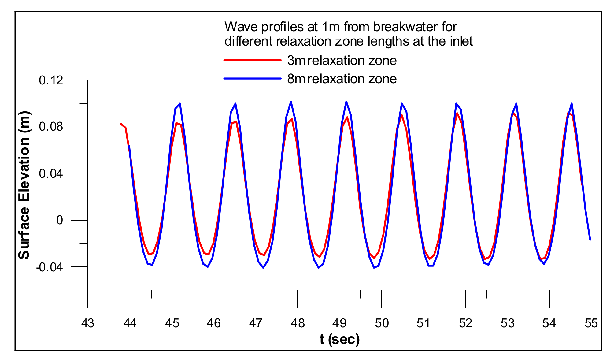
2.1.4. Wave Generation and Absorption

The additional toolbox waves2Foam [14] is used for the wave generation and absorption. Specifically, relaxation zones are implemented at the boundaries of the computational domain to prevent from any unwanted reflections. Appropriate wave theories, depending on each simulation, are implemented at the left boundary for the wave generation too.

The relaxation weighting factor $a_R$ is given by the following exponential expression:

$$a_R\left({\chi }_R\right)=1-\frac{\exp \left({\chi }_R^{3.5}\right)ibed-1}{\exp \left(1\right)-1}\gamma \iota \alpha {\chi }_R\in \left[0;1\right]$$

(10)

The weighting factor is then used to define the velocity or surface elevation by the following equation:

$$\phi =a_R{\phi }_{computed}+\left(1-a_R\right){\phi }_{target}$$

(11)

where $\phi$ is the velocity or γ (VOF method).

2.2. Morphodynamic Model

As mentioned above, the morphodynamic model has been developed in FORTRAN by the authors. The new code follows previous, similar works from Karambas and Koutitas [24] and Karambas [25] for Boussinesq models, where semi-empirical formulae, along with the sediment continuity equation, were implemented. The main difference between this model and Boussinesq models is that all accurate hydrodynamic characteristics obtained from the 3D OpenFOAM model (surface elevation, velocities, turbulent kinetic energy) are used here to estimate the sediment transport rates and obtain the seabed morphology evolution, while Boussinesq models are 2DH models which make use of semi-empirical equations (e.g., for undertow or energy dissipation). Moreover, Camenen and Larson [17] equations are implemented here, which take into account the wave asymmetry, splitting up the wave period into two separate time periods, with positive and negative orbital velocities respectively and calculating the sediment transport rates accordingly for each one of them. Furthermore, the sheet flow inception is described along with the associated phase-lag effect, which takes into account the time period that the sediment stays in suspension near the bed. Specifically, when flow switches to the opposite direction, sediment in suspension is carried away by the flow to the opposite direction too. The model takes into account the wave-current interaction too, although no current is applicable in this work. Once the sediment transport rates are calculated, the sediment mass continuity equation is applied, and the new seabed morphology is obtained. Complex geometry or steep slopes are taken into account through Watanabe coefficient [26], which is applied in the conservation of sediment transport equation. Avalanching is also incorporated in the model, although it was not used here, as the seabed is considered flat. The discretisation was made using the finite difference method (FDM).

It is well known that the sediment transport rates calculation can be divided into the bedload and the suspension load transport rates calculation. Camenen and Larson [17] proposed semi-empirical formulae for both as follows.

2.2.1. Bed Load and Sheet Flow

The bed load is given by the following equations Camenen and Larson [17], taking into account wave and current interaction:

$${\Phi }_b=\left\{\begin{array}{c}\frac{q_{sb,w}}{\sqrt{\left(s-1\right)g{D}_{50}^3}}=a_w\sqrt{{\theta }_{cw,net}}{\theta }_{cw,m}\exp \left(-b\frac{{\theta }_{cr}}{{\theta }_{cw}}\right)\\ \frac{q_{sb,n}}{\sqrt{\left(s-1\right)g{D}_{50}^3}}=a_n\sqrt{{\theta }_{cn}}{\theta }_{cw,m}\exp \left(-b\frac{{\theta }_{cr}}{{\theta }_{cw}}\right)\end{array}\right.$$

(12)

where ${\theta }_{cr}$, ${\theta }_{cw,m}$, ${\theta }_{cw}$, ${\theta }_{cn}$ are the critical, mean, maximum and current Shields parameters, $w$, $n$ stand for “wave” and “normal” directions respectively, $s(={\rho }_s/\rho$) is the relative density between sediment and water, g is gravitational acceleration, D₅₀ the median grain size, while $a_w$, $a_n$ and $b$ are coefficients given by Camenen and Larson [17] and ${\theta }_{cw,net}$ is calculated by the equation:

$${\theta }_{cw,net}=\left(1-a_{pl,b}\right){\theta }_{cw,on}-\left(1+{\alpha }_{pl,b}\right){\theta }_{cw,off}$$

(13)

where ${\theta }_{cw,on}$ and ${\theta }_{cw,off}$ take into account the wave asymmetry, as they are the mean values of the instantaneous Shields parameter for the two time periods that add up to the wave period T. Specifically, T_wc is the time period (part of the wave period) when the velocities are positive and corresponds to wave crest, while T_wt is the time period (part of the wave period) when the velocities are negative and corresponds to wave trough (T_w = T_wc + T_wt, in which T_w is the wave period).

The $a_{pl,b}$ coefficient accounts for the phase-lag effects [17], which was described previously as the phenomenon in which the sediment which stays in suspension when the flow changes direction, is drifted towards the opposite one. The $a_{pl,b}$ coefficient is given by:

$$a_{pl,b}=a_{onshore}-a_{offshore}$$

(14)

where $a_{onshore}$ and $a_{offshore}$ are given by:

$$a_j=\frac{v^{0.25}{U}_{wj}^{0.5}}{w_s{T}_j^{0.75}}exp\left[-{\left(\frac{U_{w,crsf}}{U_{wj}}\right)}^2\right]$$

(15)

where j switches between onshore and offshore as mentioned above, ν stands for water kinematic viscosity, U_w,crsf is the critical velocity for the initiation of the sheet flow, U_w is the wave orbital velocity and w_s the sediment fall velocity.

The critical velocity for the inception of the sheet flow is given by:

$$U_{w,cr,sf}=8,35\sqrt{\left(s-1\right)g\sqrt{D_{50}{\delta }_w}} \left(1+r_w\right)$$

(16)

where

$$r_w=\frac{U_{w,max}}{U_w}-1$$

(17)

is the wave asymmetry coefficient and $U_{w,max}$ the maximum wave orbital velocity.

The Shields parameters ${\theta }_{cw,on}$ and ${\theta }_{cw,off}$ in the Equation (13) are given by:

$${\theta }_{cw,j}=\frac{1}{2}{f}_{cw}{U}_{cw,j}^2/\left[\left(s-1\right)g{D}_{50}\right]$$

(18)

where j switches between onshore and offshore, U_cw the total wave and current velocity, f_cw the friction coefficient for the wave and current interaction. There is no current in this work, so the friction coefficient f_cw is related to the waves $\left(f_w\right)$ only and is equal to [1]:

$$f_{cw}=f_w=\exp \left[5.213{\left(\frac{k_s}{a_0}\right)}^{0.19}-5.977\right]$$

(19)

where $k_s$ is the bed roughness, which is taken equal to 2.5D₅₀ [27], while $a_0=U_{w,max}$ × T/2π is the amplitude of the orbital bottom velocity $U_{w,max}$.

Lastly, the coefficients $a_w,b,a_n$ in the main Equation (12) are given by: $a_w=6+6{\theta }_c/\left({\theta }_c+{\theta }_w\right)$, $b=4.5$ and $a_n=12$.

2.2.2. Suspended Load

The suspended load according to Camenen and Larson [17], is given by:

$$q_{ss,w}=U_{cw,net}\frac{C_R\epsilon }{w_s}\left[1-\exp \left(-\frac{w_s}{\epsilon }\right)\right]$$

(20)

$$q_{ss,n}=U_{c}sin\phi \frac{C_R\epsilon }{w_s}\left[1-\exp \left(-\frac{w_s}{\epsilon }\right)\right]$$

(21)

where $C_R$ is the bed reference concentration, ε the sediment diffusivity, and $U_{cw,net}$, the net mean current.

The bed reference concentration according to Camenen and Larson [17], is given by:

$$c_R=A_{cR}{\theta }_{cw,m}exp\left(-b_w\frac{{\theta }_{cr}}{{\theta }_{cw}}\right)$$

(22)

where

$$A_{cR}=3,5·{10}^{-3}\exp \left(-0,3D_{*}\right)$$

(23)

where $D_{*}$ is the dimensionless grain size given by:

$$D_{*}=\sqrt[3]{\left(s-1\right)g/v^2}{D}_{50}$$

(24)

The sediment diffusivity ε is calculated through the energy dissipation:

$$\epsilon ={\left(\frac{D_{dis}}{\rho }\right)}^{1/3}{D}_{50}$$

(25)

where $D_{dis}$ the energy dissipation, which is calculated from the OpenFOAM hydrodynamic model and specifically the turbulence model. This is one of the main differences between using the hydrodynamic OpenFOAM model and the Boussinesq model or other depth-averaged models, where the energy dissipation is calculated from semi-empirical formulae.

Lastly, the net mean current $U_{cw,net}$ is given by:

$$U_{cw,net}=\left(1-a_{pl,s}\right)U_{cw,onshore}+\left(1+a_{pl,s}\right)U_{cw,offshore}$$

(26)

where the $a_{pl,s}$ coefficient is related to the phase lag effect according to the Equation (14) with the difference in the subscript which now is s (suspended) and $U_{cw,onshore}$, $U_{cw,offshore}$ the velocities for the different parts of the wave period according to the notation described in the Section 2.2.1.

2.2.3. Conservation of Sediment Transport

The total sediment transport rate is the addition of bedload and suspended load transport rates as presented above. Once the total sediment transport rate is calculated, the new morphology of the seabed can be achieved using the conservation of sediment transport Equation [28]:

$$\frac{\partial z_b}{\partial t}+\frac{1}{1-n}\frac{\partial }{\partial x}\left(q_{x,t}-{\epsilon }_w\mid q_{x,t}\mid \frac{\partial z_b}{\partial x}\right)+\frac{1}{1-n}\frac{\partial }{\partial y}\left(q_{y,t}-{\epsilon }_w\mid q_{y,t}\mid \frac{\partial z_b}{\partial y}\right)=0$$

(27)

where z_b is the local seabed elevation (for each cell) and q_x,t(= q_s,x + q_b,x), q_y,t (= q_s,y + q_b,y) are the total sediment transport (bedload plus suspended load) rates in x and y horizontal directions respectively. The coefficient ${\epsilon }_w$ is the slope coefficient (as mentioned above) according to Watanabe [26], which for the cases of flat seabed is equal to zero.

2.3. Coupling of the Two Models—Iterative Method

As mentioned above, the method used in this work is iterative, coupling the hydrodynamic with the morphodynamic models as many times as required until the equilibrium seabed profile is achieved. The first step is to use the initial seabed morphology as input to the OpenFoam hydrodynamic model, which runs and yields the hydrodynamic field of the flow, under any given wave conditions. These results are used as input by the morphodynamic model, which is applied and a new seabed morphology is obtained. The new morphology is used as input to the OpenFoam model for the second run and this procedure is repeated until the equilibrium state is reached.

3. Results

The model is validated against three different Xie’s [1] experiments, with two of them belonging to the “relatively fine sand” group, while the third one is classified as “relatively coarse sand” case.

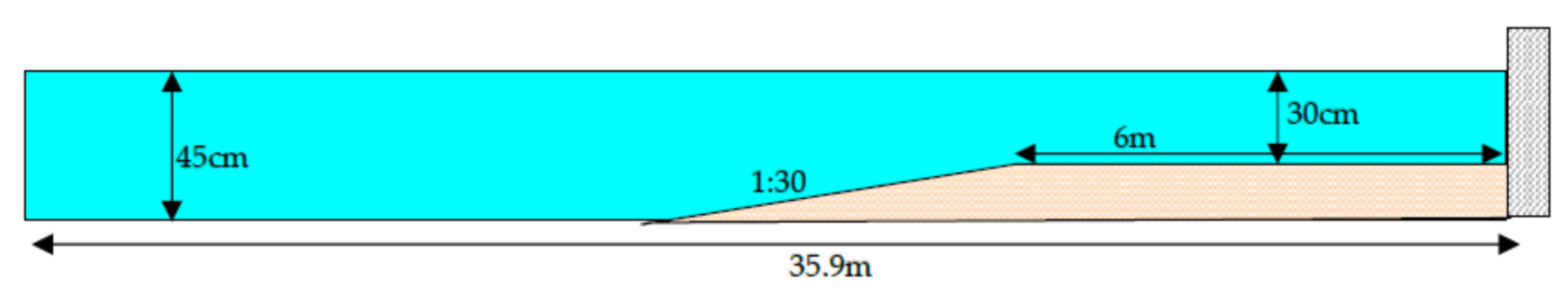
3.1. Geometry of the Model—Mesh Generation

The geometry of the model is based on the wave flume where the experiments were carried out [1]. A 38 m long numerical flume was created, with actual distance from the left boundary to the breakwater being 35.9 m, a 6 m flat sandy bed in front of the breakwater and an 1:30 slope seawards, while the depth is 0.30 m in front of the breakwater and 0.45 m in the beginning of the numerical flume. Not to scale sketch of the model’s geometry is shown in Figure 2.

The mesh was generated with standard OpenFOAM tools, specifically with blockMesh and snappyHexMesh tools, both available in OpenFOAM libraries. First of all, the basic structured mesh with same-sized computational cells was created with blockMesh and then snappyHexMesh is used to create the impermeable slope, the breakwater and the raised seabed, refining accordingly the required cells above the sandy seabed, as it cuts the numerical domain. The refinement process has been done with snappyHexMesh as described in the OpenFoam tutorial and have been studied in some works [29]. The discretization of the mesh used is Δx = 1 cm and Δz = 1 cm. Suitable boundary conditions were implemented.

3.2. Wave and Sediment Characteristics

Table 1. Wave and sediment characteristics.

Case	D50	wf	H	T	L	H/L	H/gT2	d/L	H/D50	Group
2a	106 μm	0.7 cm/s	7.5 cm	1.32 s	2.0 m	0.0375	0.0044	0.15	707.5	Fine
7a	106 μm	0.7 cm/s	5 cm	2.41 s	4.0 m	0.0125	0.0009	0.075	471.7	Fine
23a	780 μm	11 cm/s	6.5 cm	1.53 s	2.4 m	0.0271	0.0028	0.125	83.3	Coarse

shows the wave and sediment characteristics for the three implemented cases, where D₅₀ is the median grain size, w_f is the sediment fall velocity (taken from [1]), H is the wave height, T is the wave period and L is the wave length. Fifth-order Stokes regular waves were implemented for all 3 cases. The last column in Table 1 shows the classification of each case according to Xie [1] and the case numbering refers to Xie’s [1] respective experiments.

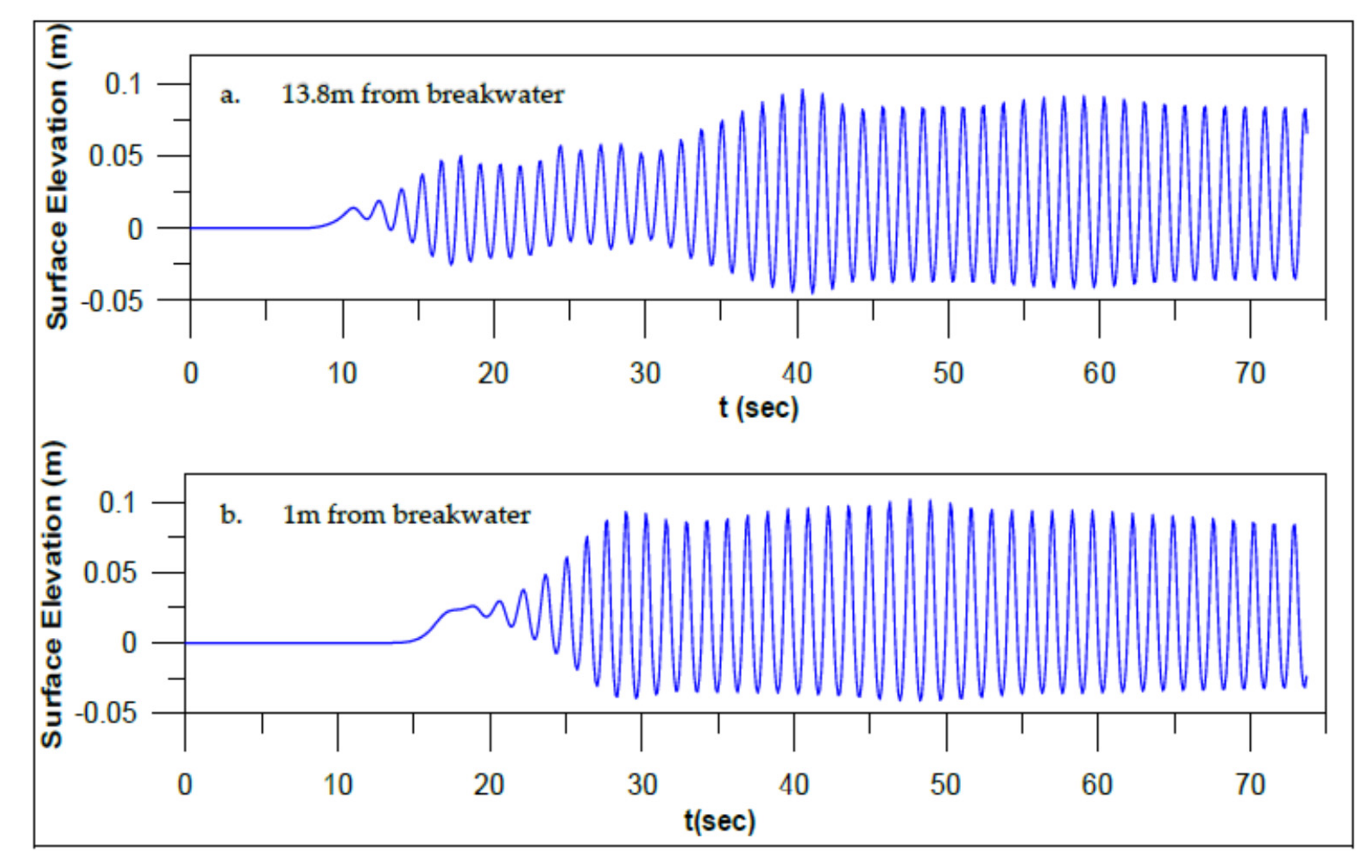
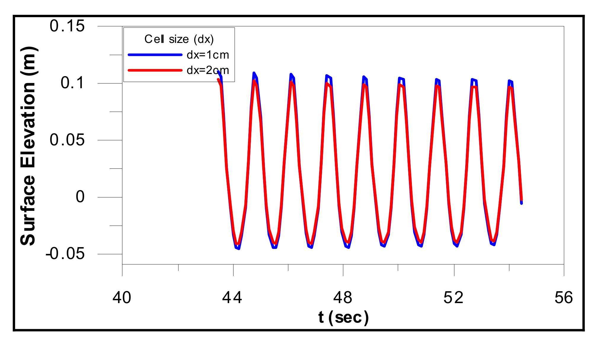
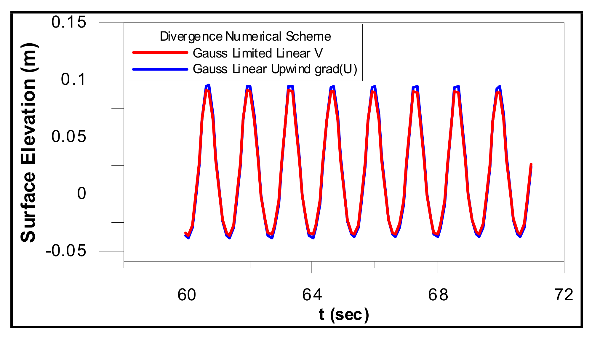
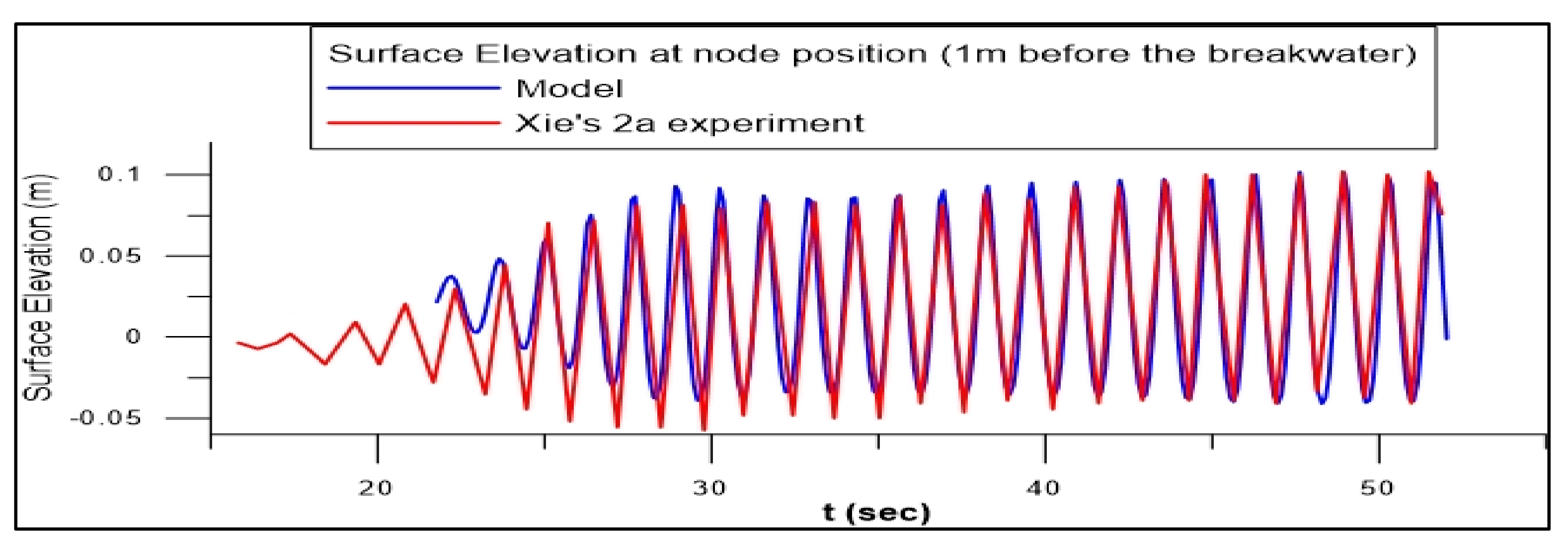
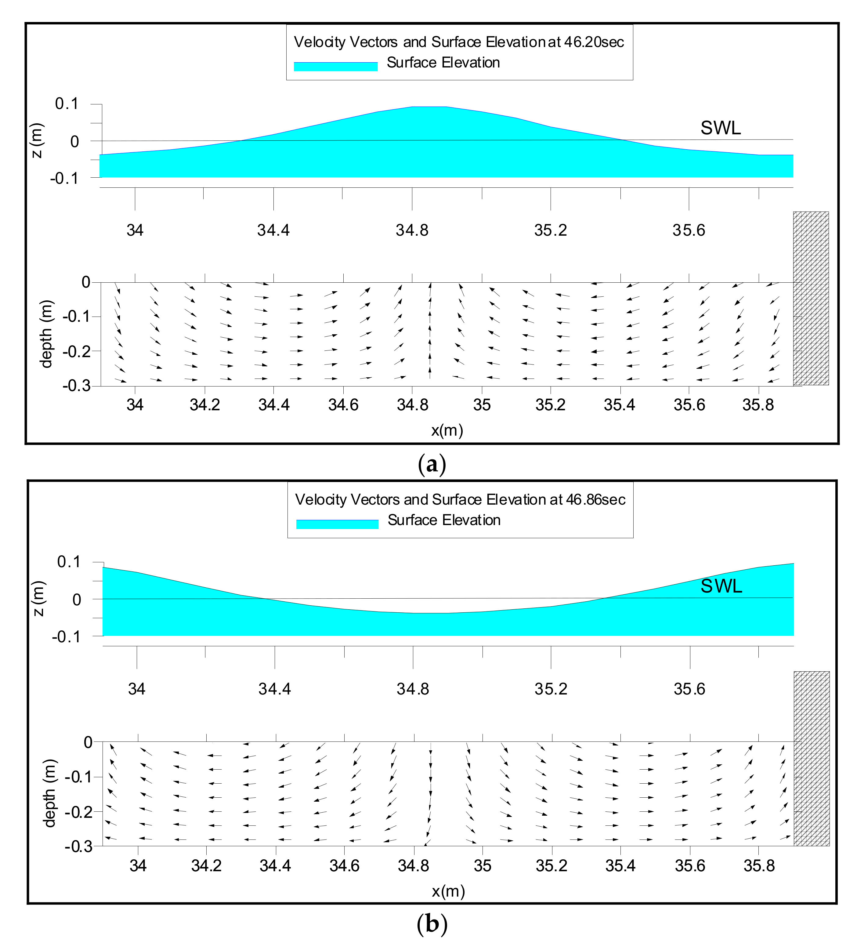
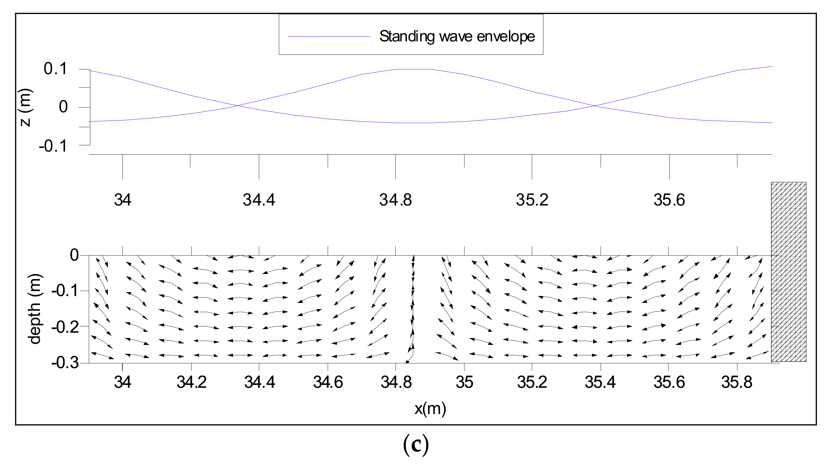
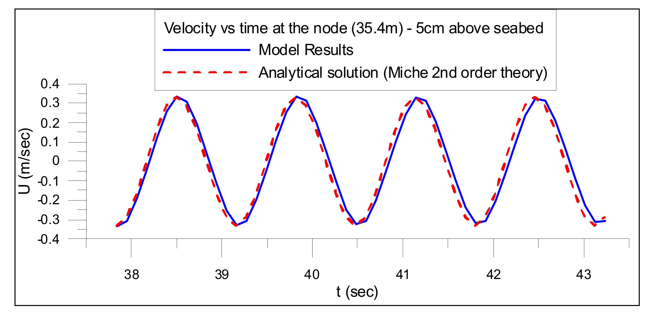
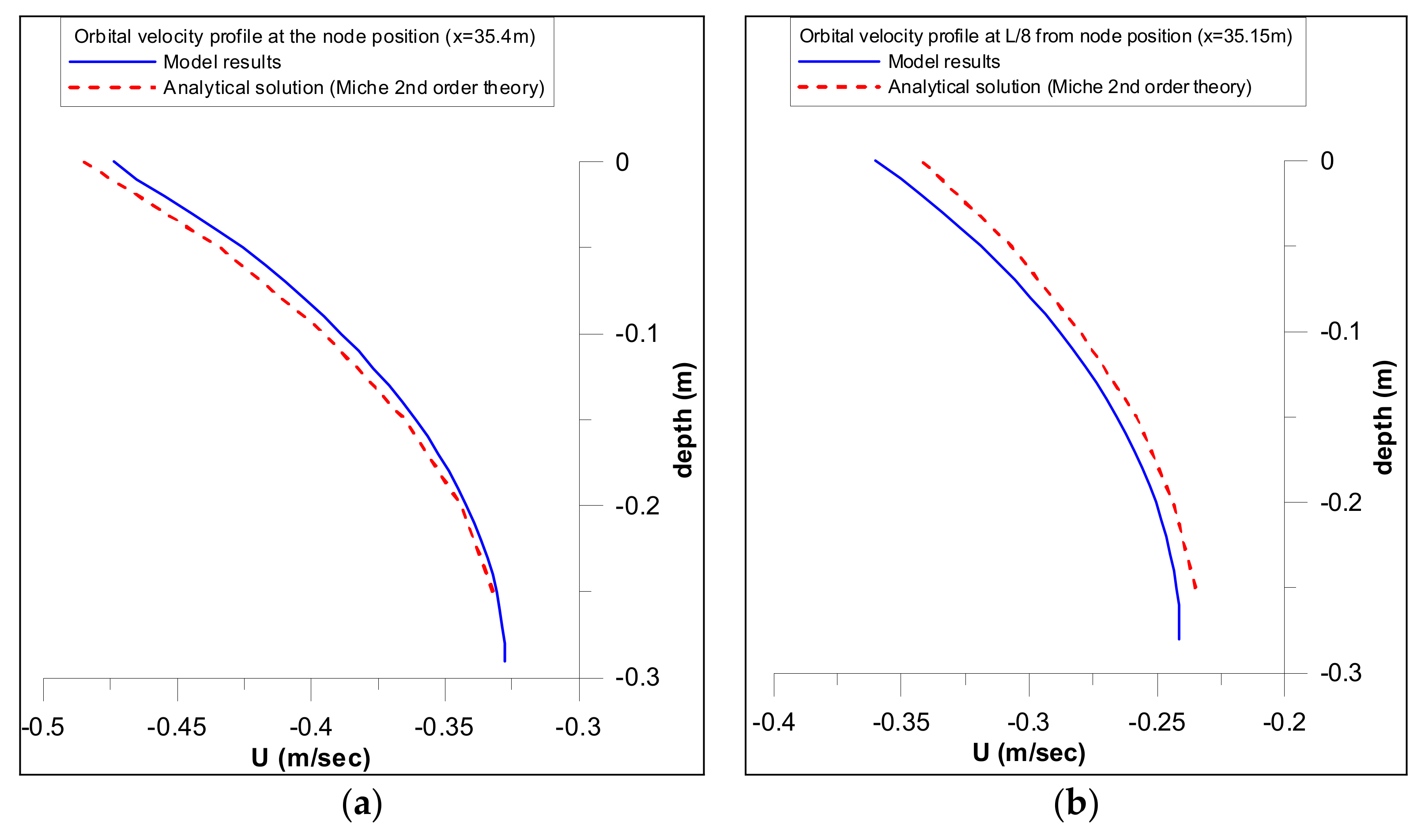
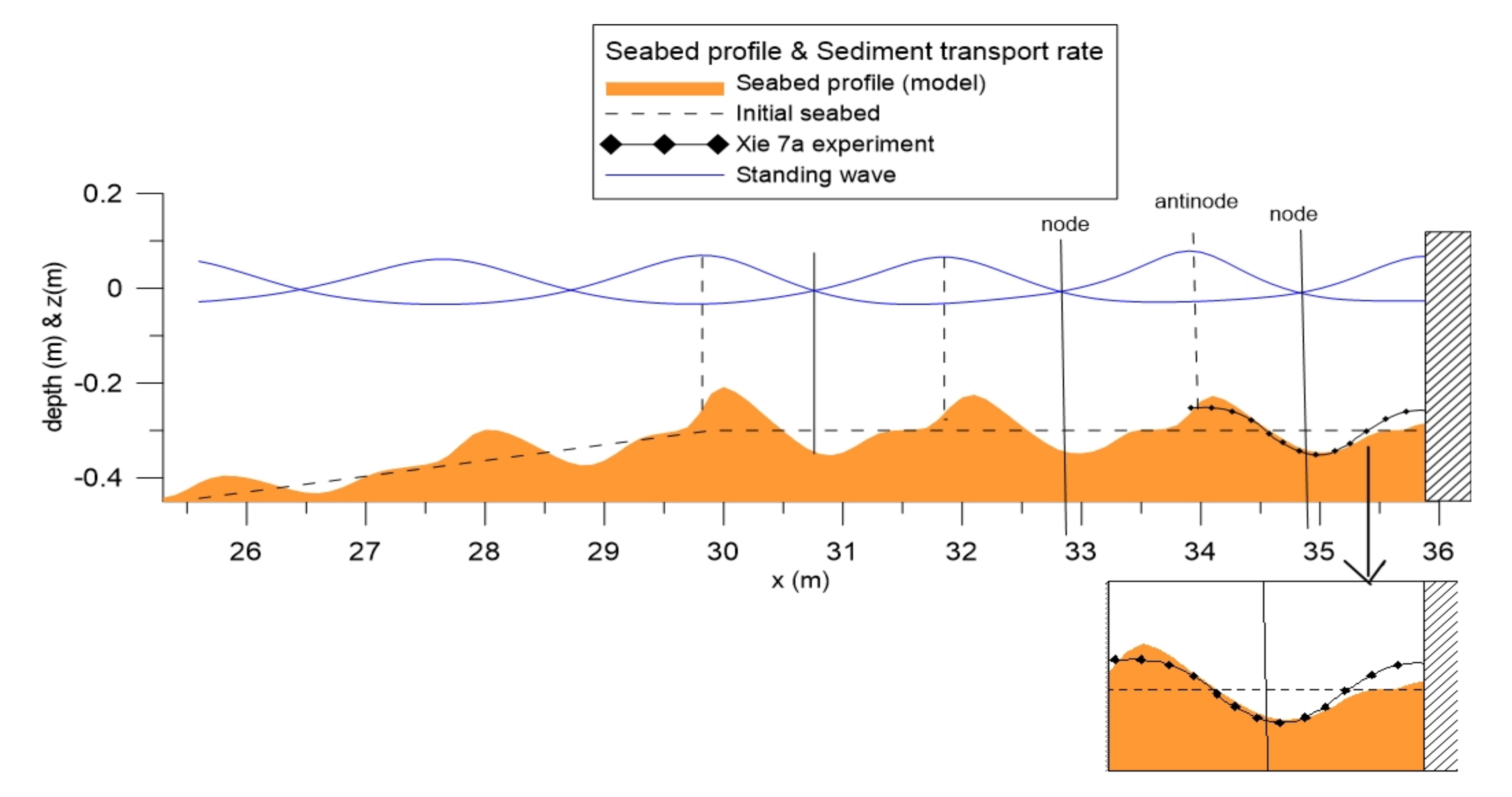
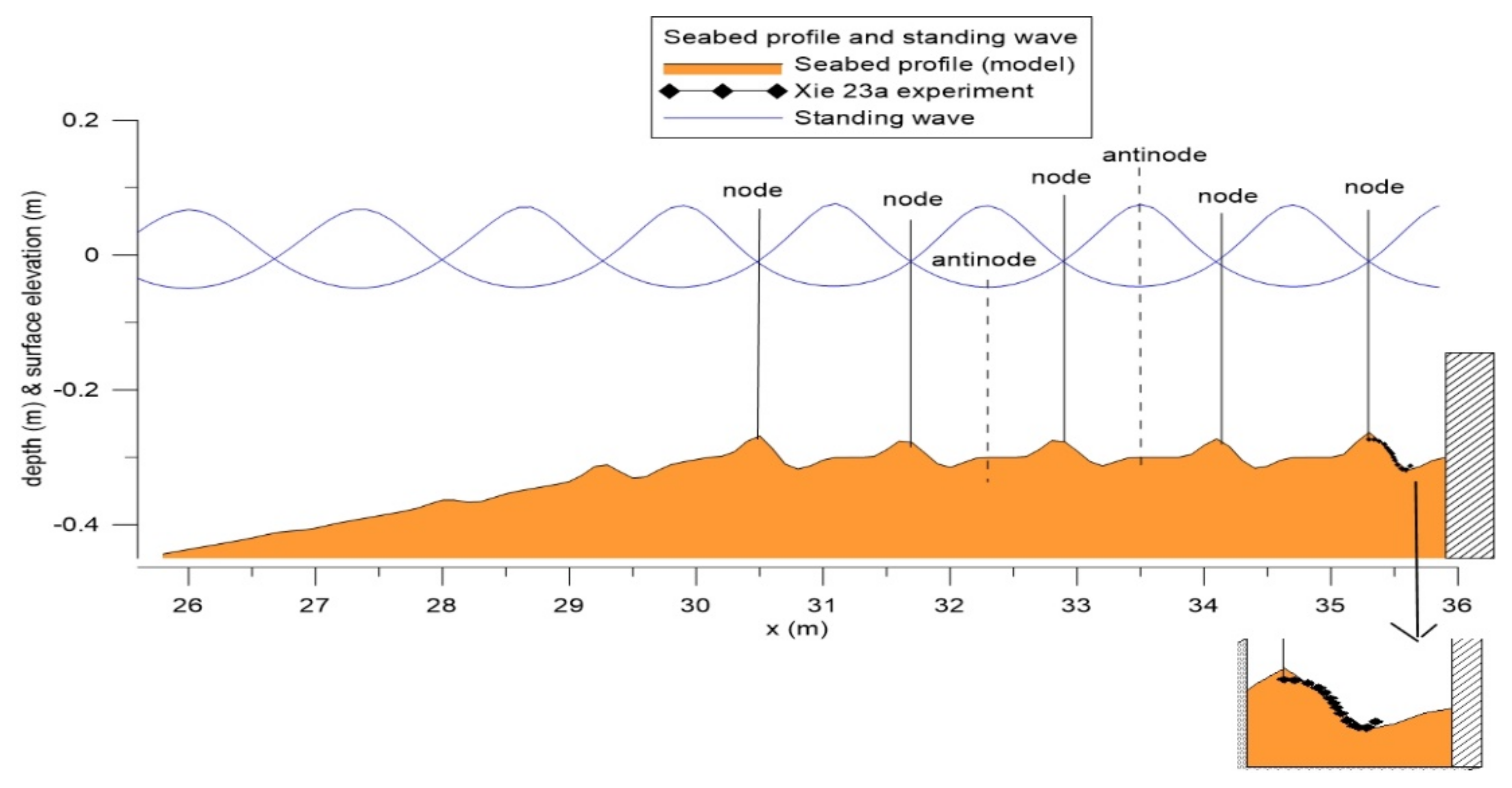
3.3. Hydrodynamic Results—Standing Wave Formation

The hydrodynamic model is being validated against Xie’s [1] 2a experiment and analytical solutions. Moreover, the performance of two different lengths of relaxation zones, two different cell sizes with respect to dx and two numerical schemes for the convection term of the Navier–Stokes equations is examined. The validation has been made for the initial seabed before any morphological changes occurred. Regular fifth-order Stokes waves have been implemented with wave height of H = 7.5 cm and period T = 1.32 s to match the wave conditions of the aforementioned experiment. The duration of the first simulation with the initial seabed was 72 s to allow for 55 waves to propagate.

Figure 3 shows the instantaneous surface elevation at two different positions, specifically at 13.8 m and 1 m from the breakwater, respectively. The transition from the incident of 7.5 cm height wave to the respective standing wave is depicted in Figure 3a. Specifically, the incident wave reaches this position (just before the slope) after 10 s, while the standing wave formation starts at about 35 s from the beginning of the simulation. There is a significant wave height increase between 35 s and 40 s, when it reaches its peak, while the standing wave takes its steady form just after 45 s. Figure 3b shows the standing wave formation just 1 m away from the wall. Due to the fact that the position is very close to the wall, the transition from incident to standing wave occurs immediately. The latter takes its steady form after 40 s from the beginning of the simulation, with the wave height being 15 cm, while it starts decreasing after 50–55 s. This can be attributed to the long simulation, as well as the long numerical flume. Moreover, the wave energy dissipation inside the domain, caused by the use of the turbulence model, also affects the wave height.

Furthermore, the role of the relaxation zones is crucial for long simulations. Figure 4 compares the wave heights at the position of 1 m before the breakwater (34.9 m from the inlet), which correspond to two different relaxation zones lengths, 3 m (1.5 × L) and 8 m (4 × L) respectively. It seems that the length of the relaxation zone affects the steadiness of the waves in long simulations. As mentioned above and shown in Figure 3b, the wave height decreases after around 55 s, which is also depicted in Figure 4, but Figure 4 also shows that in the case of 3m long relaxation zone, the wave height is significantly smaller, starting to increase and become steady after 50 s. This difference can be attributed to the long simulation, the short wave that was used in this case (T = 1.32 s) and the long numerical flume, which, can cause the accumulation of tiny unwanted reflections at the boundary when combined. The use of longer relaxation zone increases the computational cost; however, it can improve the accuracy of the results.

The discretization of the domain can affect the accuracy of the numerical results too, although this is more important in breaking waves cases, where the unsteadiness and turbulence effects require higher mesh resolution. Jacobsen [30], for example, applied an aspect ratio of 92 to produce a standing wave, while he found that the aspect ratio required to describe a wave breaker is 1. However, due to the long numerical flume in this case, as well as long -in terms of duration-simulation, higher mesh resolution is required. Two different values of dx were examined, as shown in Figure 5, where the wave heights of the cases of dx = 1 cm and dx = 2 cm at the location of 1 m away from the breakwater are depicted. It seems that the finer the mesh, the better the results, as a difference of about 1 cm–2 cm in wave height can be observed. Hence, dx = 1 cm was implemented and the respective aspect ratio dx/dz is 1.

Another factor which can affect the results is the divergence numerical scheme for the convection term of the RANS equations, as this term defines at which rate the velocity U changes in space. Two numerical schemes were tested, both available in OpenFOAM libraries, the Gauss limited linear V [31], where a limiter is applied in the direction of greater change and the Gauss linear Upwind grad (U) [32], which is an upwind scheme with a correction depending on the cell gradient. Figure 6 shows the comparison between the wave heights that obtained for these two schemes respectively for the last 10 s of the simulation (the last 10 s were selected, so that the effect of the numerical scheme can be shown). It can be observed that the Gauss linear Upwind grad (U) scheme yields slightly better results, especially in long (in duration) simulations and is implemented here.

Following the implementation of the above configurations, the model was applied, and surface elevation numerical results were compared with Xie’s experimental data (2a experiment) [1]. Figure 7 shows the comparison between computed and experimental results, which seems to be in good agreement, especially after 35 s, when steadiness is reached.

Figure 3 shows the formation of the standing wave at two different positions, just before the slope and 1 m away from the breakwater. The velocity distribution is depicted in Figure 8a,b at two different time instances and at distance of 1 wave length from the breakwater. The nodes close to the breakwater, are formed at the positions of around 35.4 m and 34.4 m, while the antinode at the position of 34.85 m. The velocity distribution follows exactly the surface elevation results, with the velocity vectors being horizontal at the position of the nodes and vertical at the antinode, while they have opposite directions at these two different instants, following the surface elevation’s oscillation. Figure 8c shows the standing wave envelope and the total particle movement, as it can be derived from the velocity vectors directions. Further to the qualitative observation, the horizontal components of velocities are compared with second-order theory of Miche:

$$U_{w,x}=\frac{2\pi H}{T}\frac{\cosh (k\left(z+d\right)}{\sinh \left(kd\right)}coskx cos\omega t+\frac{3{\pi }^2}{2T}\frac{H^2}{L}\frac{\cosh (2k\left(z+d\right)}{{\sinh }^4\left(kd\right)}sin2kx sin\omega t$$

(28)

where $U_{w,x}$ is the horizontal orbital velocity, k = 2π/L the wavenumber, ω = 2π/T the angular frequency, x = 0 at the position of the node and positive towards the breakwater, z the surface elevation with z = 0 at Still Water Level (SWL) and positive upwards, H, L, T the wave height, length and period—respectively, d is the depth and t is the time. Figure 9 shows the comparison between model results and Miche analytical solution at the position of the node and 5 cm above the flat seabed. The numerical results are in good agreement with Miche second-order theory.

Moreover, according to Xie’s [1] experimental data, the maximum value for the horizontal velocity is 0.328 m/s, while model’s maximum value at this position is 0.332 m/s (Figure 9), which is in agreement with theory. The orbital velocity profiles are also compared with Miche analytical solution in Figure 10 at the node position and L/8 from the node position. The numerical results are in good agreement with analytical solution at the bottom at the node position, while slightly deviate towards the free surface (the difference is <0.01 m/s). There is also a slight deviation between numerical results and analytical solution at L/8 from the node position, with the model yielding higher values in this instance (circa 0.01 m/s).

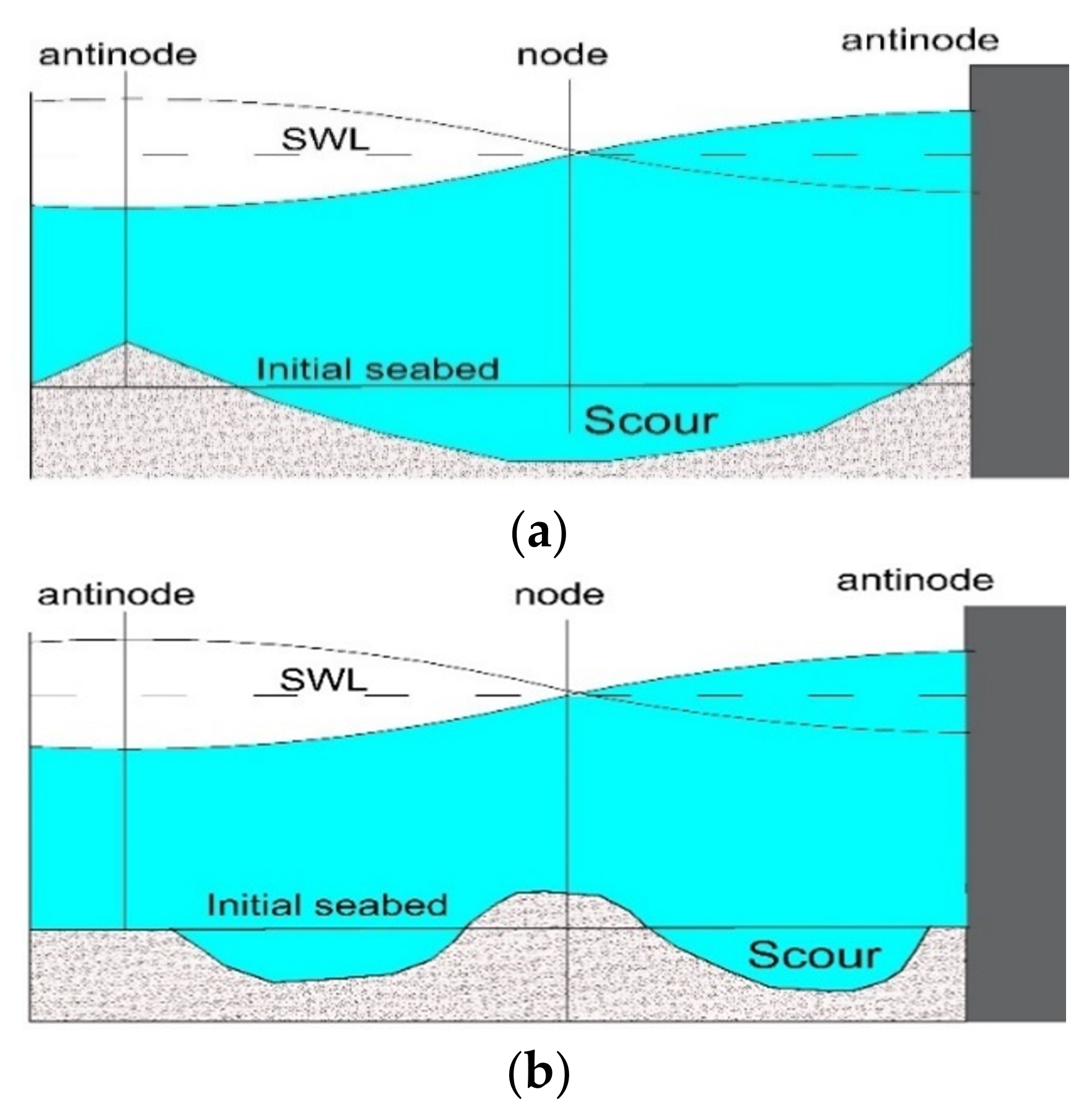
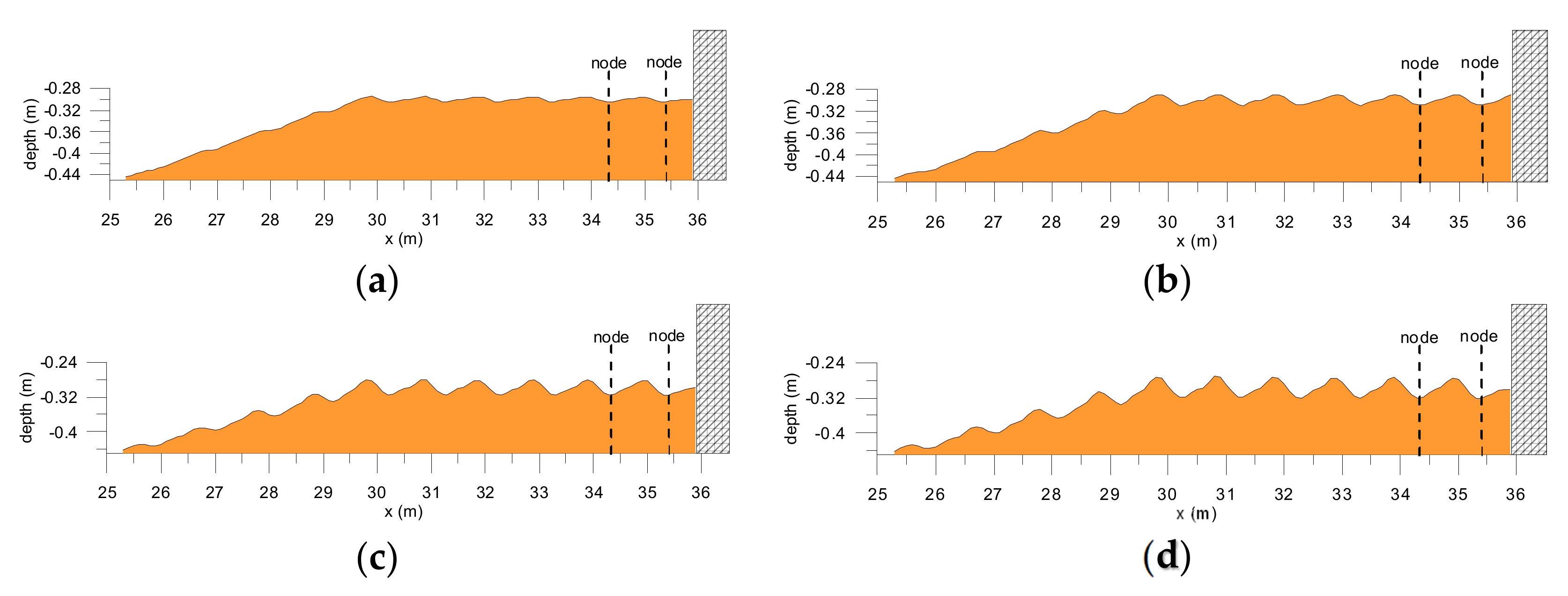
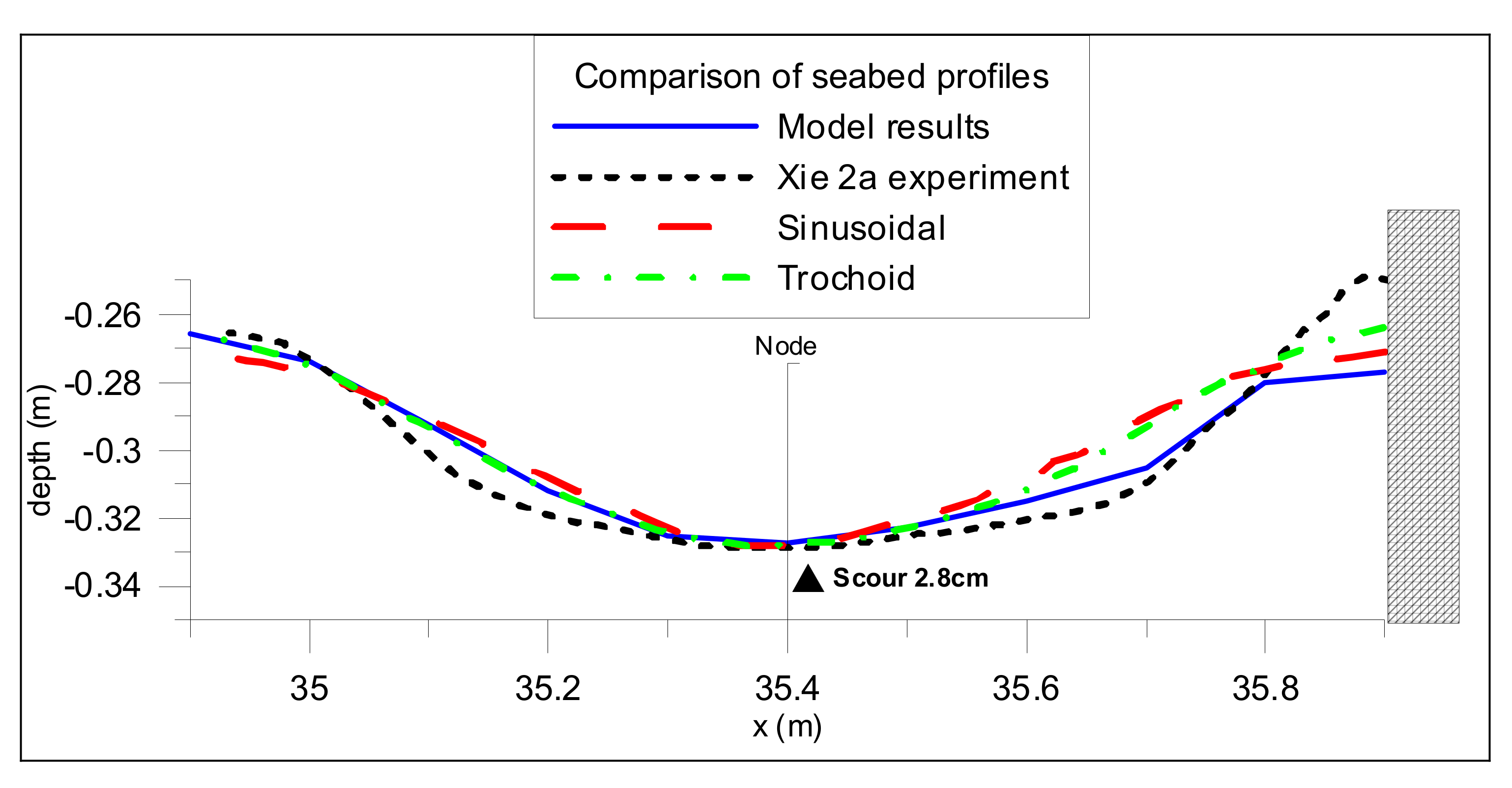
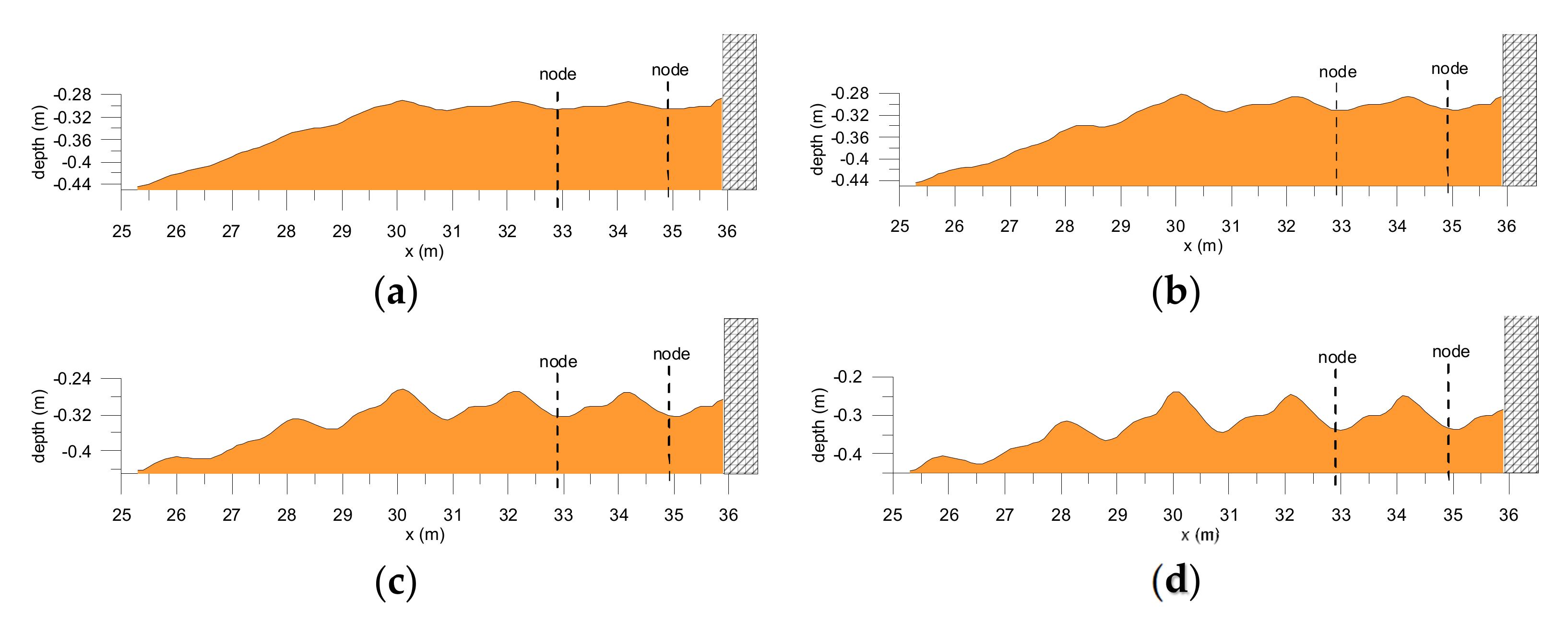
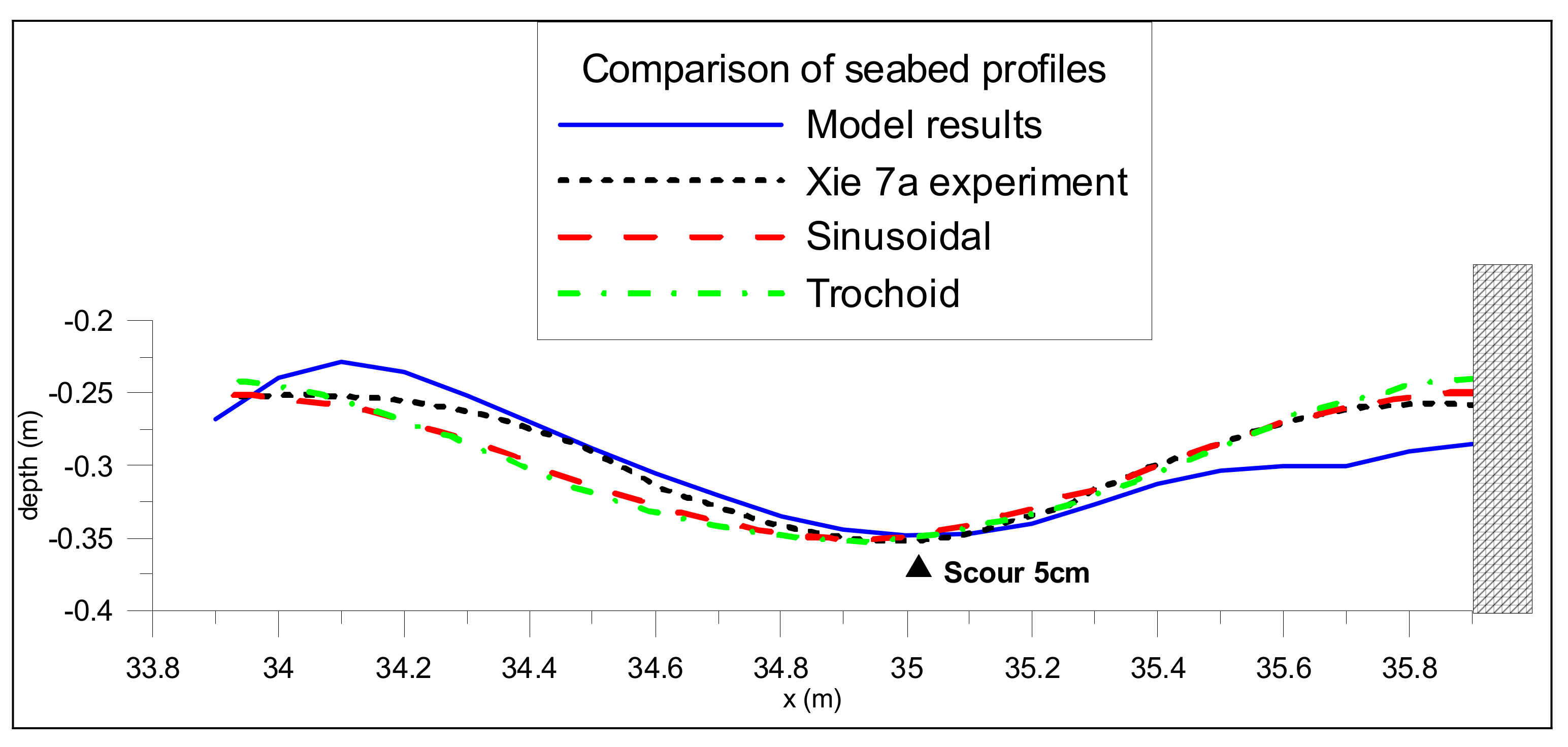
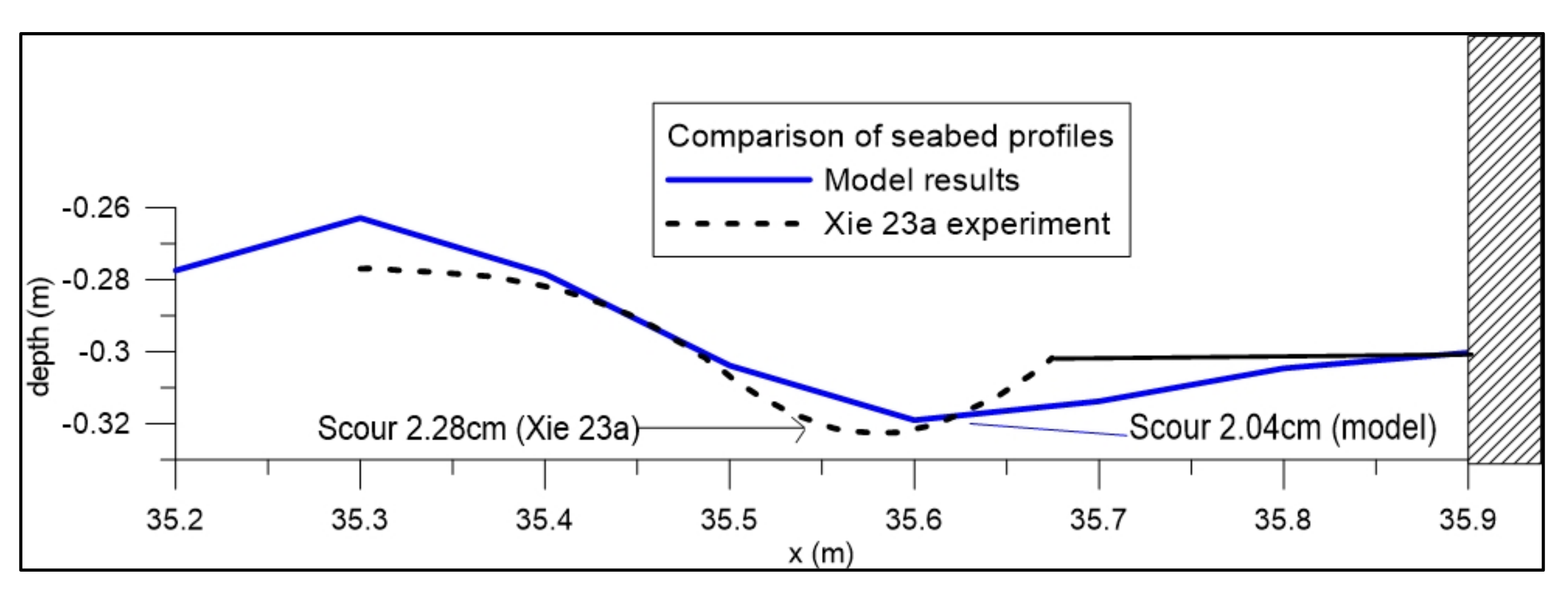
3.4. Morphodynamic Results—Scouring Depth and Scouring Patterns

The morphodynamic model is applied and couples the hydrodynamic solution to produce the sediment transport rates and update the seabed morphology, based on the sediment continuity, in an iterative process. Figure 11 shows the seabed profile evolution for 2a test, at 4 different instants. According to Table 1 and Xie [1], this test belongs to the “relative fine sand” group, where scour is expected at node positions and deposition at antinodes, which seems to be the case here, as the computed scouring pattern follows this rule.

The first two nodes close to the wall are marked with dashed lines (35.4 m and 34.4 m, respectively) in Figure 11 for all four instants, and it seems that this scouring pattern of alternating scour with deposition at nodes and antinodes respectively remains the same at all times during the simulation of test 2a. Ripples are created in the whole length of the sandy bottom under the influence of the standing waves. The equilibrium profile is shown in Figure 12 along with the standing wave. It can easily be observed that the equilibrium seabed profile is in complete agreement with the “relative fine sand” scouring pattern, as scour occurs at the nodes and deposition at the antinodes. Furthermore, the numerical results are compared satisfactorily with experimental data [1] with regards to the local scour in front of the breakwater.

Figure 13 further compares the numerical results for the scouring depth in front of the breakwater with Xie [1] experimental data, as well as sinusoidal and trochoid curves as per Xie [1] comparison. All these curves agree on the scouring depth, which is 2.8 cm, as predicted by the model.

The next test, 7a, concerns a longer wave (double wavelength) in the same wave flume, meaning that the depth in front of the breakwater is still 30 cm. The iterative method of coupling the two models was applied and the seabed morphology evolution during this process is depicted in Figure 14 for four different time instants. The nodes close to the wall are marked with dashed lines and found at the positions 34.9 m and 32.9 m, respectively. The standing wave is depicted in Figure 15. It seems that the model results are in agreement with Xie’s [1] classification, as the scour is formed at the nodes and the deposition at the antinodes, which is a typical “relative fine sand” pattern.

Although the pattern is followed as expected, it seems that there is a slight shift between the antinode, which is close to 32 m and the top of the ridge. A slight shift exists at the positions of the other antinodes as well, but the one close to 32 m is slightly bigger. This can be attributed to the bigger wave length (L = 4 m) with respect to the length of the sandy flat bed, which is 6 m, as there is the slope before the flat bed that can affect the standing wave evolution. This might not happen if the wave length was multiple of the flat bed length. Moreover, comparing the results of 2a and 7a experiments, it can be noticed that in the latter case, a small “berm” is created between the node and the antinode. This can be attributed to the bigger wave length too, as the scouring hole is getting too big to stand alone with a uniform shape, which does not affect the position of the scour though. In terms of comparison between numerical results and experimental data, it can be observed from Figure 15 that they are in good agreement.

This can also be attested by Figure 16, where the numerical results for the scouring depth and scouring pattern are compared with Xie experimental data [1], sinusoidal and trochoid curves. It seems that they are in good agreement; however, the model’s deposition next to the wall is smaller than the experimental one. The scour depth was predicted 5 cm by the model, which is consistent with the other three curves.

The above two tests are classified as “relative fine sand” cases, while the next test 23a belongs to the “relative coarse sand” group according to Xie [1]. Figure 17 shows the seabed evolution at four different time instants, while the nodes positions are marked with dashed lines. The main difference in the scouring pattern can be easily identified, if Figure 17 is compared with Figure 11 and Figure 14. In previous cases, scour was formed at nodes positions, while the opposite is observed in this case. Ridges are formed at the nodes’ positions, as expected, in line with Xie [1] classification.

Figure 1 shows the standing wave evolution, while the nodes close to the breakwater can be identified at the positions 35.3 m and 34.1 m, respectively. The antinodes are marked with dashed lines and the nodes with solid lines. The scouring pattern, as depicted in Figure 18, is consistent with Xie’s [1] scouring pattern for “relative coarse sand”, as well as Sumer and Fredsoe [2]. The scour is formed between the nodes and the antinodes, while a small ridge is formed at the antinodes position as shown in Sumer and Fredsoe, whose elevation can be even lower than the initial one [2]. However, the scour is formed differently next to the antinodes. The scour that is formed seawards is fully developed, while the scour that is formed towards the breakwater is barely identified. Apart from that, the numerical results are in agreement with the relative coarse sand scouring pattern. The experimental data [1] are limited for “relative coarse sand” tests; however, the maximum scour depth and an indicative scouring curve were available for this test [1].

Figure 19 shows the comparison between numerical results and Xie’s available experimental data. The scour according to the experimental data is 2.28 cm, while the model’s prediction is 2.04 cm. Also, model’s seabed profile slightly underestimates the scour depth and slightly overestimates the deposition at the node position (35.3 m). According to Xie [1], there is a length from the antinode towards the node (22 cm in this instance), where the seabed remains practically intact (this length is shown with black solid line in Figure 19). Numerical results are also in good agreement with experimental data in this instance.

4. Discussion

Following the description and application of the coupled model, some interesting points can be further discussed in this section, as derived from the simulation process and the numerical results.

As pointed out above, the turbulence model, the wave generation and absorption method, the numerical scheme of the RANS equations convection term, as well as the mesh resolution, are crucial for the successful set-up of the hydrodynamic model. The k-w SST was selected following previous authors’ works [15,18,33], as it seems that prevails over the rest on the OpenFOAM platform, with the quick note that the density term needs to be included in the equations, so that the free surface cells are defined correctly. The wave generation and absorption method and its implementation is also important especially for long (in time) simulations and long numerical domains, as it is the case in this instance. The selection of relaxation zones method was based on the fact that an adequate length of absorption zone must be defined, so that even tiny accumulated unwanted reflections would not contaminate the results. Two different lengths (3 m and 8 m) of relaxation zones were tested and as expected, the latter one prevailed over the short one. The implementation of the numerical scheme for the convection term of the RANS equations is another factor that can have an impact on the results, as it defines the rate at which the velocity changes in space. The Gauss linear upwind grad (U) scheme [32] seems to behave better in this case in comparison with the Gauss limited linear V [31] one, as the latter imposes a limiter in the direction of greater change, while the former one is an upwind scheme with correction depending on the cell gradient. Their impact on the wave heights were shown and this may be attributed to the limiter imposed on the velocity gradient at the free surface cells. With regards to the mesh resolution, it seems that the smaller dx improves the results, although the aspect ratio for the production of standing waves on OpenFOAM can be very high [30].

With regards to the morphodynamic model, the code was developed by the authors implementing the Camenen and Larson formula [17] and takes into account the wave asymmetry and the initiation of the sheet flow over ripples, including the phase lag effect. That means that the velocities are calculated separately for the period that they are positive and the period that they are negative and as a sequence, the Shields parameter is calculated separately for each one of these periods too. Also, the phase lag effect coefficient is calculated separately for each one of these time periods, which improves the way that the particles in suspension near the bed are simulated. The mean velocity values in this formula are calculated as the root mean square (rms) values, therefore any zero values in case of wave symmetry are avoided. The sediment continuity Equation (27) is being solved iteratively, producing the updated seabed morphology.

Both the hydrodynamic and morphodynamic results were validated against experimental data and/or analytical solutions. The model successfully predicts the local scour in front of the breakwater, as well as the scouring pattern, including ripples in the whole domain.

The novelty of this work is the development of a numerical model, coupling an advanced CFD RANS model on OpenFOAM platform with a developed by the authors morphodynamic one, that can successfully simulate not only the local scour depth and pattern in front of vertical breakwaters, but the ripples and the scouring pattern in the whole domain too, according to the classification in the literature [1,2]. To the best of the authors’ knowledge, the existing literature includes numerical attempts that only examine the scour at a very short length (half wave length) from the breakwater. For example, Gislason et al. [9] mention there were no ripples in their model and the attempt to model them was abandoned due to numerical instabilities. Also, Hajivalie et al. [10] used an Euler–Lagrange approach, but their results are limited to only one validation case and to the local scour at a distance of a half-wavelength from the breakwater. Moreover, unlike previous works [9,10] where the numerical domain was limited to a short distance from the vertical wall, the numerical domain in this work was created according to the experiment (breakwater at 35.9 m from the wave inlet), and the numerical results include the bed formation in the whole domain. The ripples were formed according to the literature, with the scour being formed at the nodes position and the accretion at the antinodes for “relative fine sand” cases, while deposition at nodes and scour between the nodes and the antinodes are being formed for “relative coarse sand” ones.

However, there is room for improvement. Two things that have been mentioned in the Section 3.3 are that there is slight shift between the antinode and the top of the ridge in 7a test, especially in the middle of the flat bed length, which may be attributed to the wave length with respect to the flat bed length and the other thing is that in the case of “relative coarse sand”, the scour between the antinodes and the nodes (in ripples formation) towards the wall has slightly been developed, unlike the one to the opposite direction. Also, in the case of relatively coarse sand (23a), the model predicted a maximum scour of 2.04 cm, instead of 2.28 cm according to the available experimental data [1], which are limited for the “relative coarse sand” group though. Furthermore, the authors aim to extend the applicability of the coupled model to 3D cases.

5. Conclusions

A numerical approach was presented in this work, coupling an advanced CFD RANS model developed on the OpenFOAM platform with a morphodynamic one, as developed in FORTRAN by the authors. The model describes the hydrodynamic and morphodynamic processes and has been implemented here to predict the scour depth and the scouring pattern in front of a vertical breakwater.

The model has been tested against experimental data and analytical solutions for surface elevation, orbital velocities evolution near the bed, velocities profiles, velocity vectors distribution, standing wave formation, scouring pattern and ripples formation in the whole domain and local scouring depth in front of a vertical-wall breakwater. Xie’s [1] experimental data were used to validate the model and specifically tests 2a and 7a for the “relative fine sand” and 23a for the “relatively coarse sand” classifications, with model results being in good agreement with experimental data. The scour depth prediction was accurate for the tests 2a and 7a (fine sand), while it was close to the experimental data for the test 23a (coarse sand). The model accurately predicts the scouring pattern/ripples formation in the whole domain.

References

1. Xie, S.L. Scouring Patterns in Front of Vertical Breakwaters and Their Influences on the Stability of the Foundations of the Breakwaters; Delft University of Technology: Delft, the Netherlands, 1981. [Google Scholar]
2. Sumer, B.M.; Fredsøe, J. Experimental study of 2D scour and its protection at a rubble-mound breakwater. Coast. Eng. 2000, 40, 59–87. [Google Scholar] [CrossRef]
3. Carter, T.G.; Liu, L.F.P.; Mei, C.C. Mass transport by waves and offshore sand bedforms. J. Waterw. Harb. Coast. Eng. ASCE 1973, 99, 165–184. [Google Scholar]
4. Lee, K.; Mizutani, N. Experimental study on scour occuring at a vertical impermeable submerged breakwater. J. Appl. Ocean. Res. 2008, 30, 92–99. [Google Scholar] [CrossRef]
5. Mei, C. The Applied Dynamics of Ocean Surface Waves; World Scientific: Hackensack, NJ, USA, 1989. [Google Scholar]
6. Bing, C. The numerical simulation of local scour in front of a vertical-wall breakwater. J. Hydrodyn. 2007, 18, 134–138. [Google Scholar]
7. Gislason, K.; Fredsøe, J.; Mayer, S.; Sumer, B.M. The mathematical modeling of the scour in front of the toe of a rubble-mound breakwater. In Book of Abstracts, Proceedings of the 27th International Coastal Engineering Conference, Sydney, Australia, 16–21 July 2000; ASCE: Reston, VA, USA, 2000; Volume 1, p. 1. [Google Scholar]
8. Gislason, K.; Fredsøe, J.; Sumer, B.M. Flow under standing waves Part 1. Shear stress distribution, energy flux and steady streaming. Coast. Eng. 2009, 56, 341–362. [Google Scholar]
9. Gislason, K.; Fredsøe, J.; Sumer, B.M. Flow under standing waves. Part 2. Scour and deposition in front of breakwaters. Coast. Eng. 2009, 56, 363–370. [Google Scholar] [CrossRef]
10. Hajivalie, F.; Yeganeh-Bakhtiary, A.; Houshanghi, H.; Gotoh, H. Euler-Lagrange model for scour in front of vertical breakwater. Appl. Ocean Res. 2012, 34, 96–106. [Google Scholar] [CrossRef]
11. Engelund, F.A.; Fredsøe, J. A sediment transport model for straight alluvial channels. Nord. Hydrol. 1976, 7, 293–306. [Google Scholar] [CrossRef] [Green Version]
12. Karagiannis, N.; Karambas, T.; Koutitas, C. Numerical simulation of scour in front of a breakwater using OpenFoam. In Proceedings of the 4th IAHR Europe Congress, Liege, Belgium, 27–29 July 2016; pp. 309–315. [Google Scholar]
13. Karagiannis, N.; Karambas, T.; Koutitas, C. Numerical simulation of scour pattern and scour depth prediction in front of a vertical breakwater using OpenFoam. In Proceedings of the 27th International Ocean and Polar Engineering Conference (ISOPE 2017), San Francisco, CA, USA, 25–30 June 2016; Volume 3, pp. 1342–1348. [Google Scholar]
14. Jacobsen, N.G.; Fuhrman, D.R.; Fredsøe, J. A Wave generation toolbox for the open-source CFD library: OpenFoam. Int. J. Numer. Methods Fluids 2012, 70, 1073–1088. [Google Scholar] [CrossRef]
15. Karagiannis, N. An Advanced Numerical Model Fully Describing the Hydro-and Morphodynamic Processes in the Coastal Zone. Ph.D. Thesis, Civil Engineering Department, Aristotle University of Thessaloniki, Thessaloniki, Greece, 2019. [Google Scholar]
16. Hirt, C.W.; Nichols, B.D. Volume of fluid (VOF) method for the dynamics of free boundaries. J. Comput. Phys. 1981, 39, 201–225. [Google Scholar] [CrossRef]
17. Camenen, B.; Larson, M. A Unified Sediment Transport Formulation for Coastal Inlet Application; Technical report ERDC/CHL CR-07-1; US Army Engineer Research and Development Center: Vicksburg, MS, USA, 2007. [Google Scholar]
18. Karagiannis, N.; Karambas, T.; Koutitas, C. Numerical simulation of wave propagation in surf and swash zone using OpenFoam. In Proceedings of the 26th International Ocean and Polar Engineering Conference, Rhodes, Greece, 26 June–2 July 2016; Volume 3, pp. 1342–1348. [Google Scholar]
19. Higuera, P.; Lara, J.L.; Losada, I.J. Realistic wave generation and active wave absorption for Navier–Stokes models: Application to OpenFOAM. Coast. Eng. 2013, 71, 102–118. [Google Scholar] [CrossRef]
20. Jasak, H. Error Analysis and Estimation for the finite Volume Method with Applications to Fuid Fows. Ph.D. Thesis, Deptartment of Mechanical Engineering, Imperial College of Science, Technology and Medicine, London, UK, 1996. [Google Scholar]
21. Rusche, H. Computational fluid Dynamics of Dispersed Two-Phase flows at High Phase Fractions. Ph.D. Thesis, Department of Mechanical Engineering, Imperial College of Science, Technology & Medicine, London, UK, 2003. [Google Scholar]
22. Menter, F.R. Zonal Two Equation k-ω Turbulence Models for Aerodynamic Flows. AIAA Paper 1993, 1993–2906. [Google Scholar] [CrossRef]
23. Menter, F.R. Two-equation eddy-viscosity turbulence models for engineering applications. AIAA J. 1994, 32, 1598–1605. [Google Scholar] [CrossRef] [Green Version]
24. Karambas, T.; Koutitas, C. Surf and swash zone morphology evolution induced by nonlinear waves. J. Waterw. Port Coast. Ocean. Eng. 2002, 128, 102–113. [Google Scholar] [CrossRef]
25. Karambas, T.V. Design of detached breakwaters for coastal protection: Development and application of an advanced numerical model. In Proceedings of the 33rd International Conference on Coastal Engineering, Santander, Spain, 1–6 July 2012. [Google Scholar]
26. Watanabe, A. Modeling of sediment transport and beach evolution. In Nearshore Dynamics and Coastal Processes; Horikawa, K., Ed.; University of Tokyo Press: Tokyo, Japan, 1998; pp. 292–302. [Google Scholar]
27. Nielsen, P. Some Basic Concepts of Wave Sediment Transport; Series Paper 20; Institute of Hydrodynamics and Hydraulic Engineering (ISVA); Technical University of Denmark: Lyngby, Denmark, 1979. [Google Scholar]
28. Leont’yev, I.O. Numerical modelling of beach erosion during storm event. Coast. Eng. 1996, 29, 187–200. [Google Scholar] [CrossRef]
29. Gisen, D. Generation of a 3-D Mesh Using SnappyHexMesh Featuring Anisotropic Refinement and Near-Wall Layers; ICHE: Hamburg, Germany, 2014. [Google Scholar]
30. Jacobsen, N.G. A Full Hydro-And Morphodynamic Description of Breaker Bar Development. Ph.D. Thesis, Department of Mechanical Engineering, Technical University of Denmark, Lyngby, Denmark, 2011. [Google Scholar]
31. Sweby, P.K. High resolution schemes using flux-limiters for hyperbolic conservation laws. SIAM J. Numer. Anal. 1984, 21, 995–1011. [Google Scholar] [CrossRef]
32. Warming, R.F.; Beam, M.M. Upwind second-order difference schemes and applications in aerodynamic flows. AIAA J. 1976, 14, 1241–1249. [Google Scholar] [CrossRef]
33. Karagiannis, N.; Karambas, T.; Koutitas, C. Wave overtopping numerical simulation using OpenFoam. In Proceedings of the 36th IAHR World Congress, The Hague, The Netherlands, 28 June–3 July 2015. [Google Scholar]
Figure 1. Scour patterns for: (a) relatively fine sand and (b) relatively coarse sand.
Jmse 08 00836 g001
Figure 2. Sketch of the model geometry.
Jmse 08 00836 g002
Figure 3. Surface Elevation at 2 different locations. (a) 13.8 m from the breakwater, just before the slope, where the transition from incident to standing wave is shown. (b) 1 m from the breakwater where fully standing wave formation is depicted.
Jmse 08 00836 g003
Figure 4. Comparison between different relaxation zones lengths.
Jmse 08 00836 g004
Figure 5. Comparison between wave heights at location 1 m away from the breakwater for different cell sizes (different dx).
Jmse 08 00836 g005
Figure 6. Comparison between wave heights at location 1 m away from the breakwater for different divergence numerical scheme for the convection terms of RANS equations.
Jmse 08 00836 g006
Figure 7. Instantaneous Surface Elevation at the position of 1 m before the breakwater. Comparison between model results and experimental data.
Jmse 08 00836 g007
Figure 8. (a) Surface Elevation and particle velocity distribution at 46.2 s (model results for t = 35 *T). (b) Surface Elevation and particle velocity vectors at 46.53 s (model results for t = 35T + T/2). (c) Standing wave envelope and particle movement (model results).
Jmse 08 00836 g008aJmse 08 00836 g008b
Figure 9. Orbital velocity at the position of the node (35.4 m from the inlet of the flume) at 5 cm above the seabed. Comparison between numerical results and analytical solution (Miche second-order theory).
Jmse 08 00836 g009
Figure 10. Orbital velocity profiles (a) at the position of the node (35.4 m from the inlet of the flume), and (b) L/8 from the position of the node (35.15 m from the inlet of the flume). Comparison between numerical results and Miche second-order analytical solution.
Jmse 08 00836 g010
Figure 11. Seabed profile evolution after (a) 200 s, (b) 400 s, (c) 800 s, (d) 1400 s (test 2a).
Jmse 08 00836 g011
Figure 12. Final numerical seabed profile and standing wave. Comparison with experimental data (test 2a).
Jmse 08 00836 g012
Figure 13. Seabed profiles and scouring depth—comparison between model results and experimental data/theory (test 2a).
Jmse 08 00836 g013
Figure 14. Seabed profile evolution after (a) 500 s, (b) 1000 s, (c) 2000 s, (d) 3800 s (test 7a).
Jmse 08 00836 g014
Figure 15. Final numerical seabed profile and standing wave—Comparison with experimental data (test 7a).
Jmse 08 00836 g015
Figure 16. Seabed profiles and scouring depth-comparison between model results and experimental data/theory (test 7a).
Jmse 08 00836 g016
Figure 17. Seabed profile evolution after (a) 500 s, (b) 800 s, (c) 1500 s, (d) 3200 s (test 23a).
Jmse 08 00836 g017
Figure 18. Final numerical seabed profile and standing wave—Comparison with experimental data (test 23a).
Jmse 08 00836 g018
Figure 19. Seabed profiles and scouring depth—Comparison between model results and experimental data (test 23a).
Jmse 08 00836 g019