Wave Interaction with Single and Twin Vertical and Sloped Slotted Walls


Abstract
1. Introduction
2. Materials and Methods
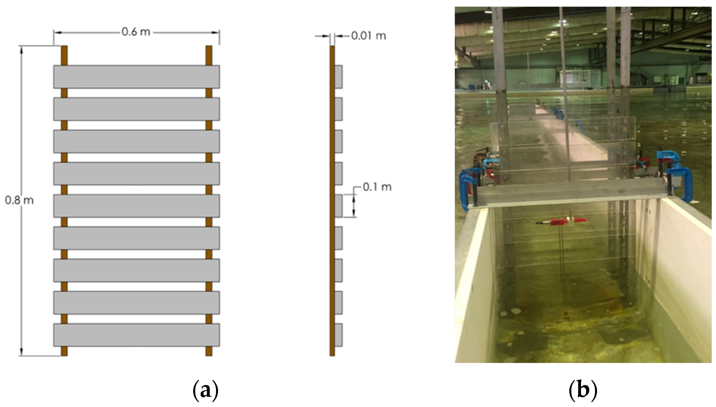
2.1. Model Specifications
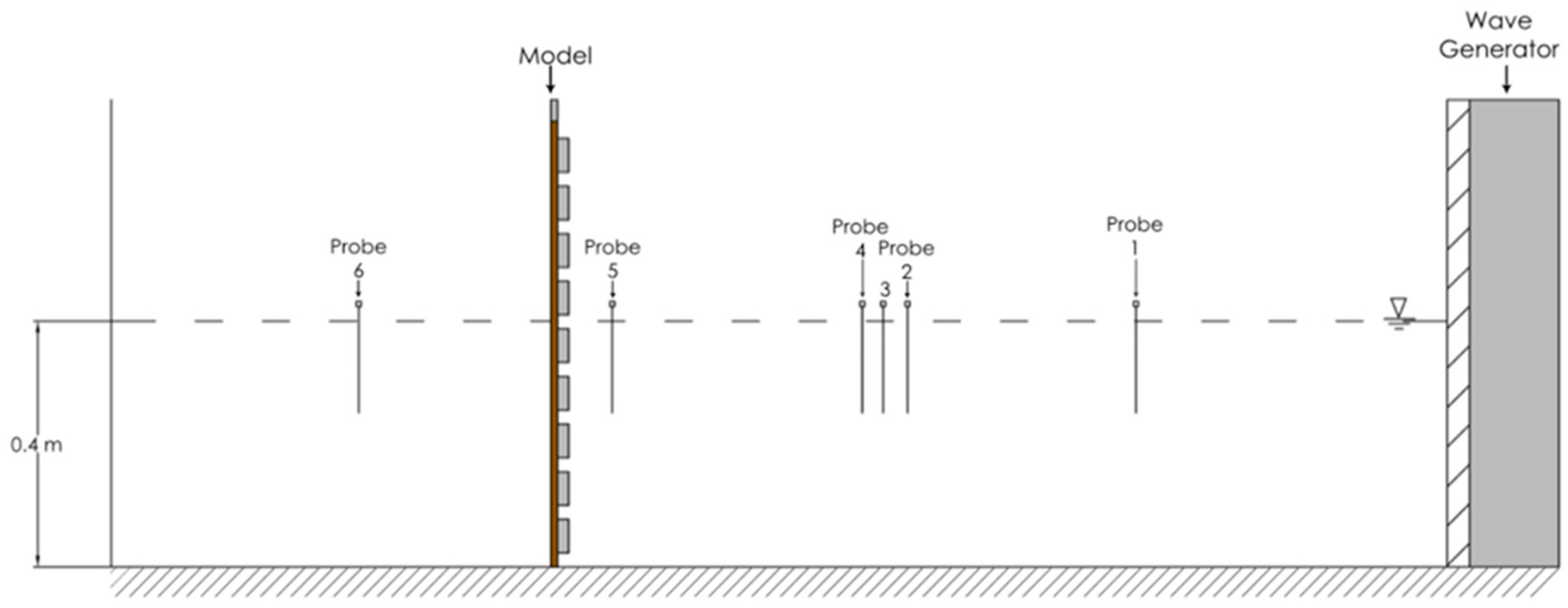
2.2. Testing Facilities
2.3. Wave Specifications
3. Results and Discussion
3.1. General
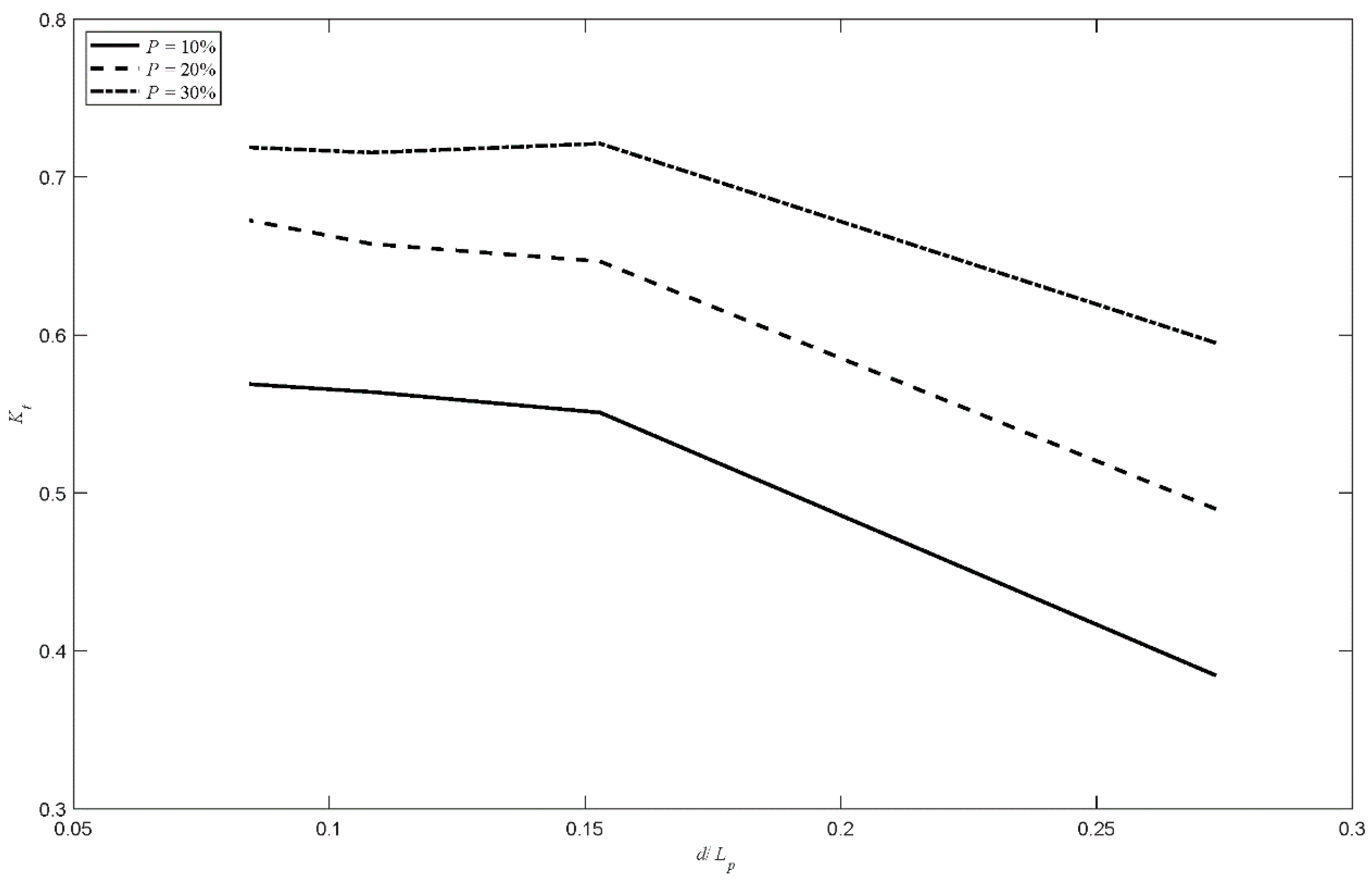
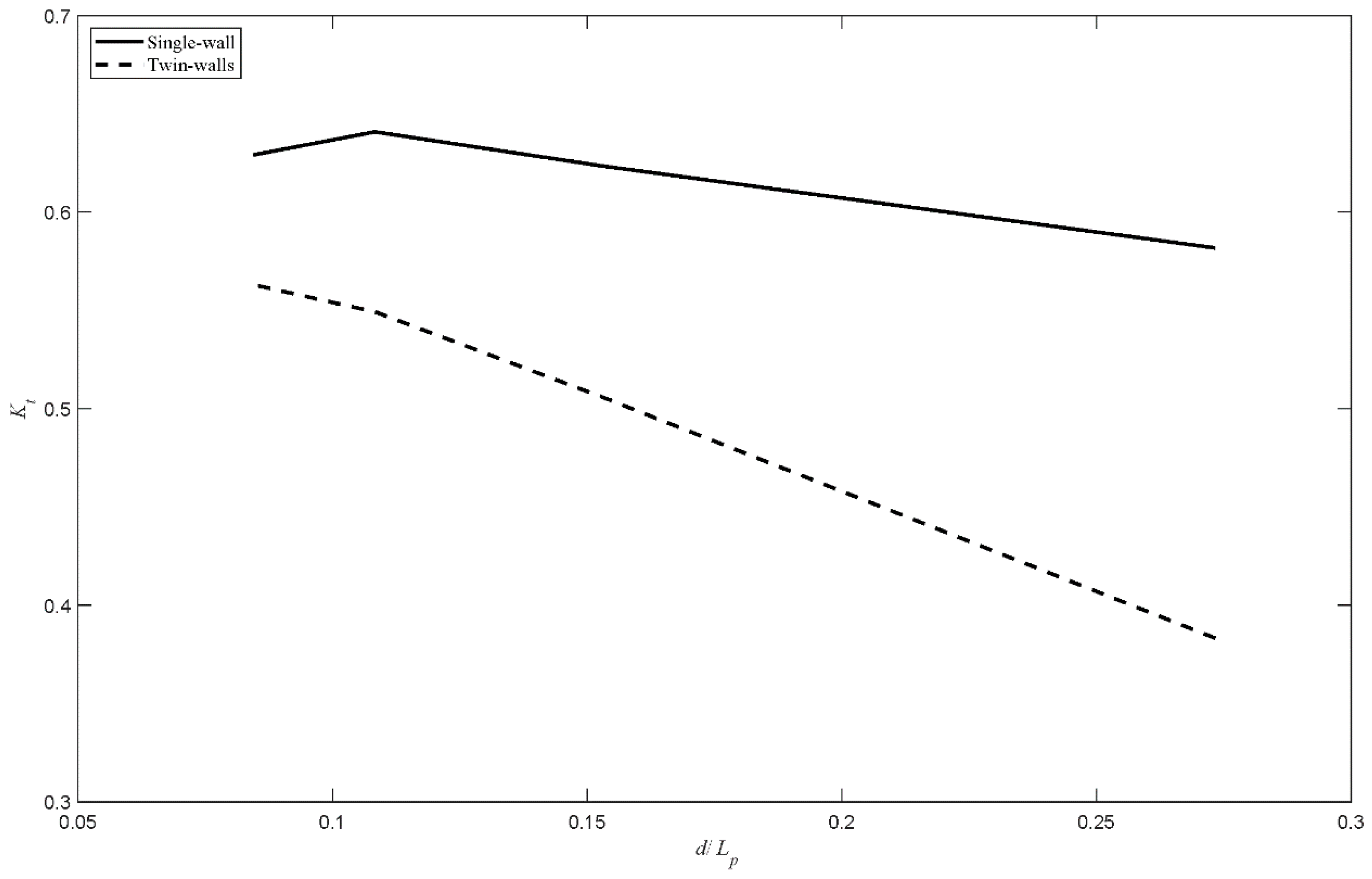
3.2. Wave Transmission Coefficient, Kt
3.2.1. Effect of Porosity
3.2.2. Effect of Number of Walls
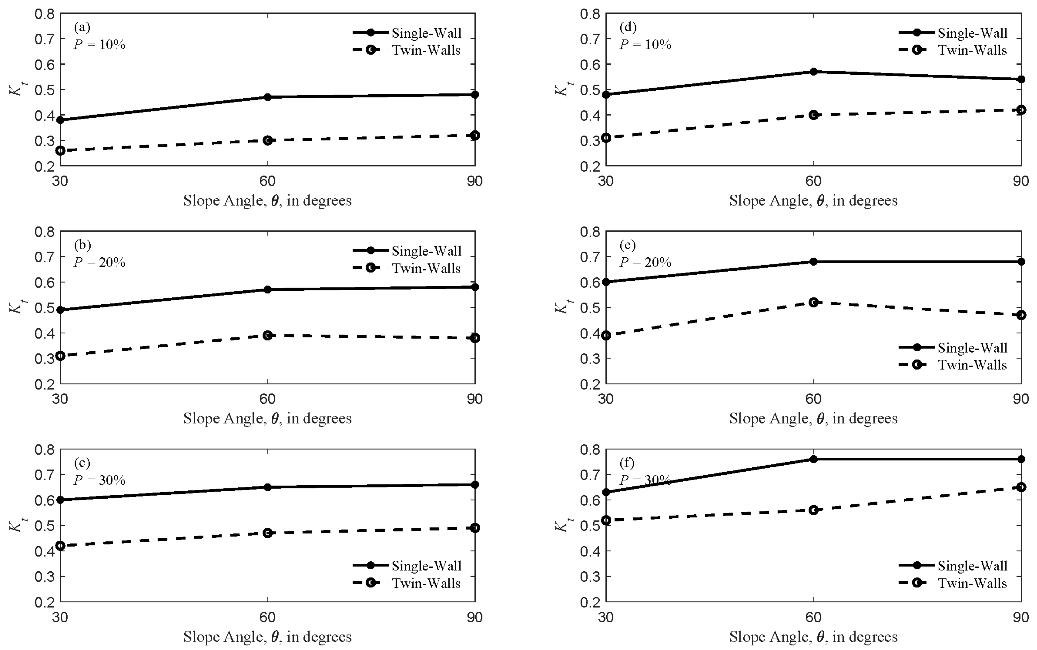
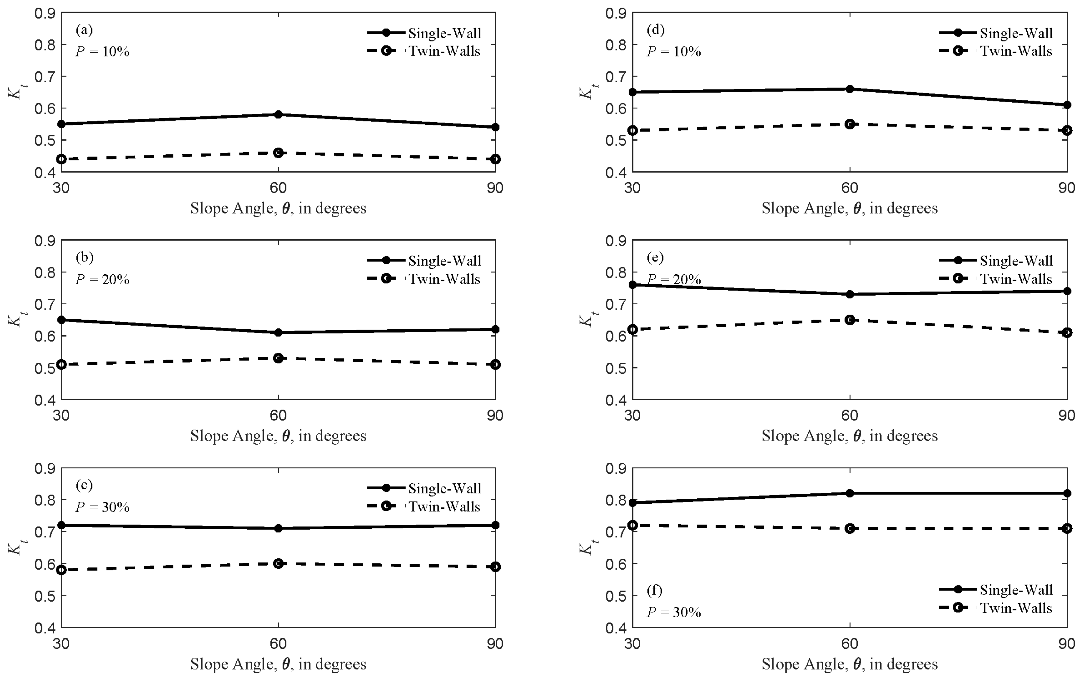
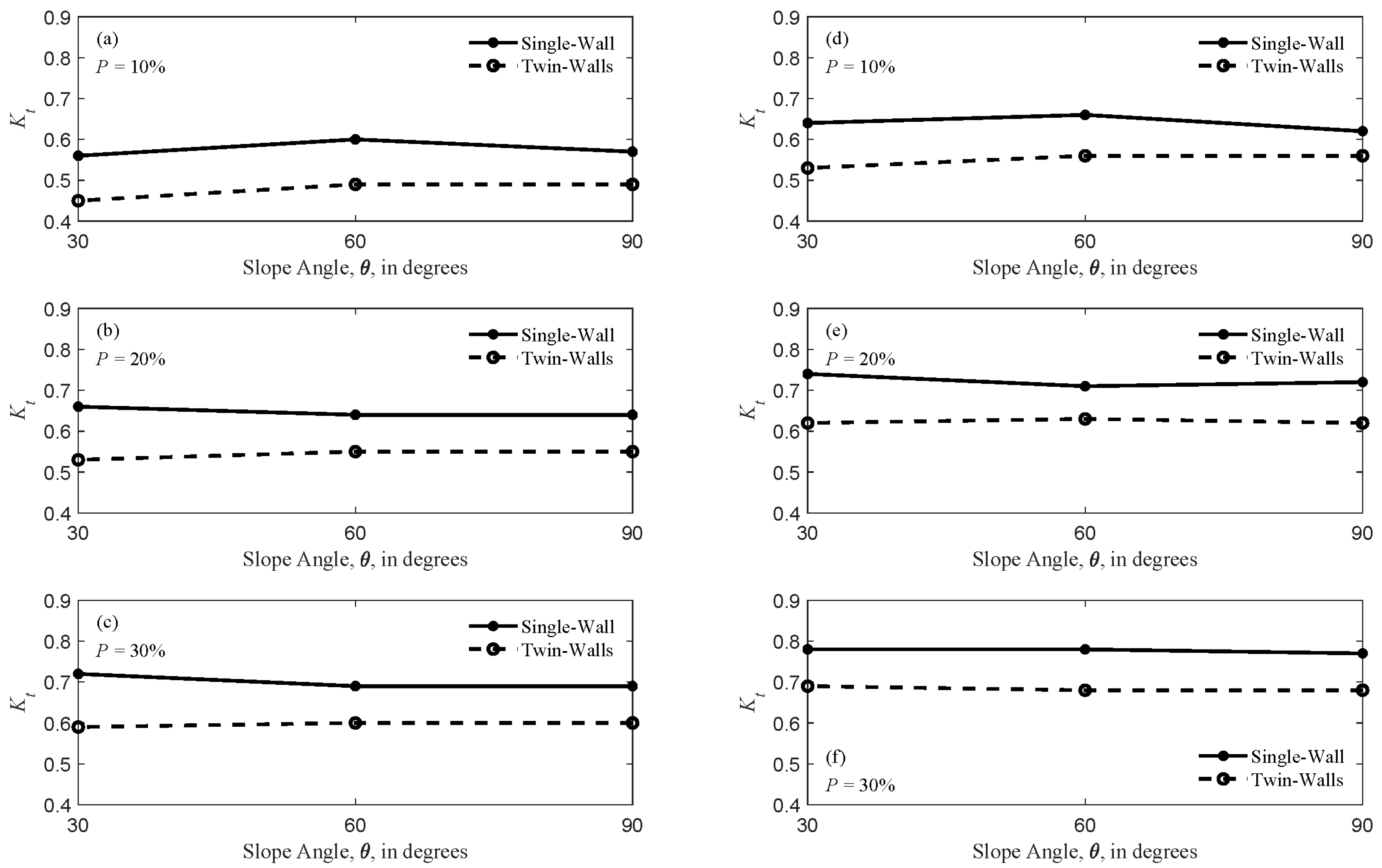
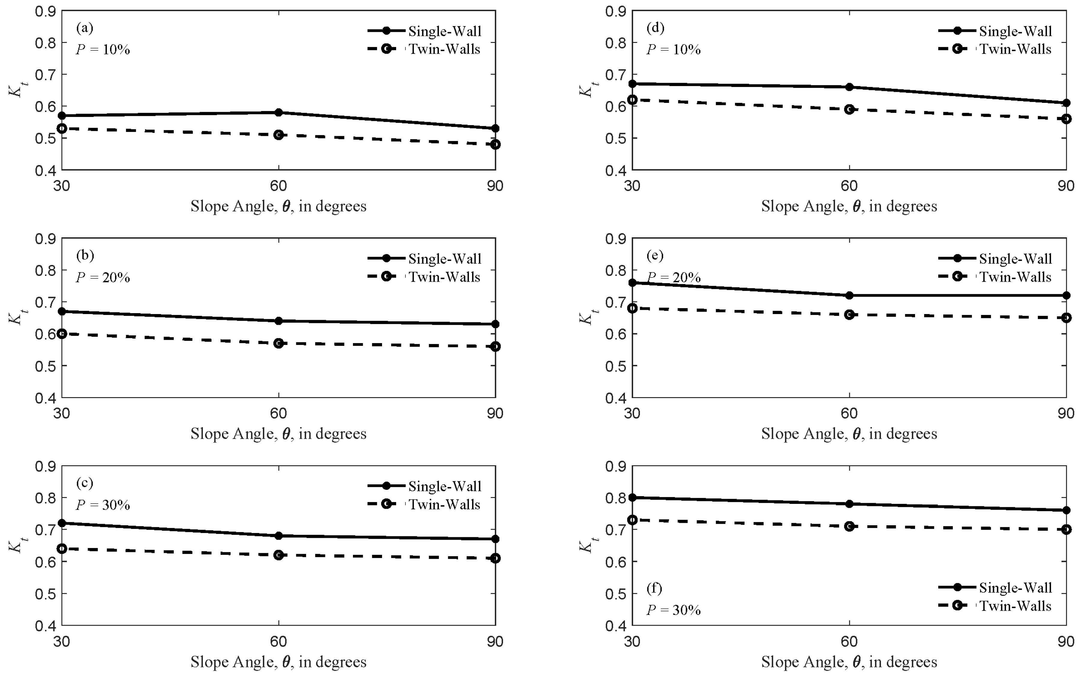
3.2.3. Effect of Slope Angle
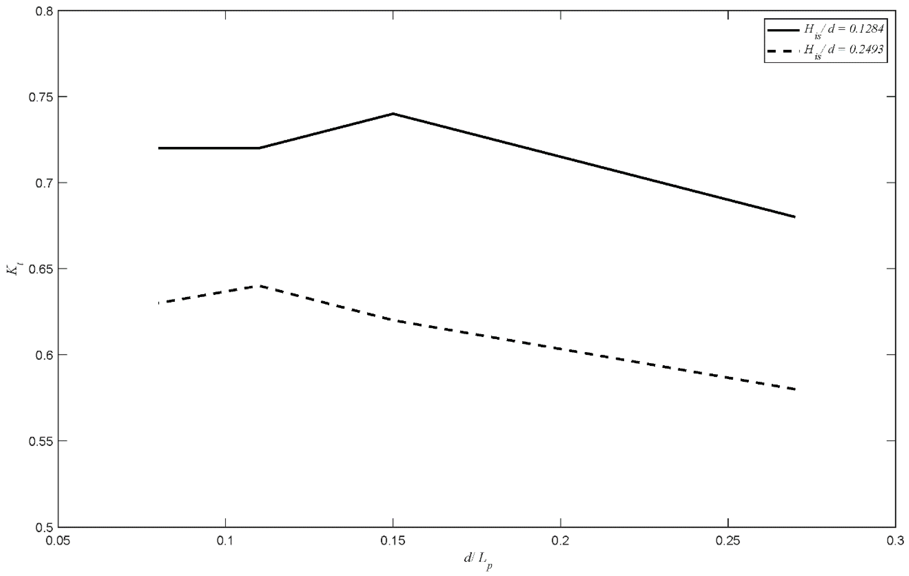
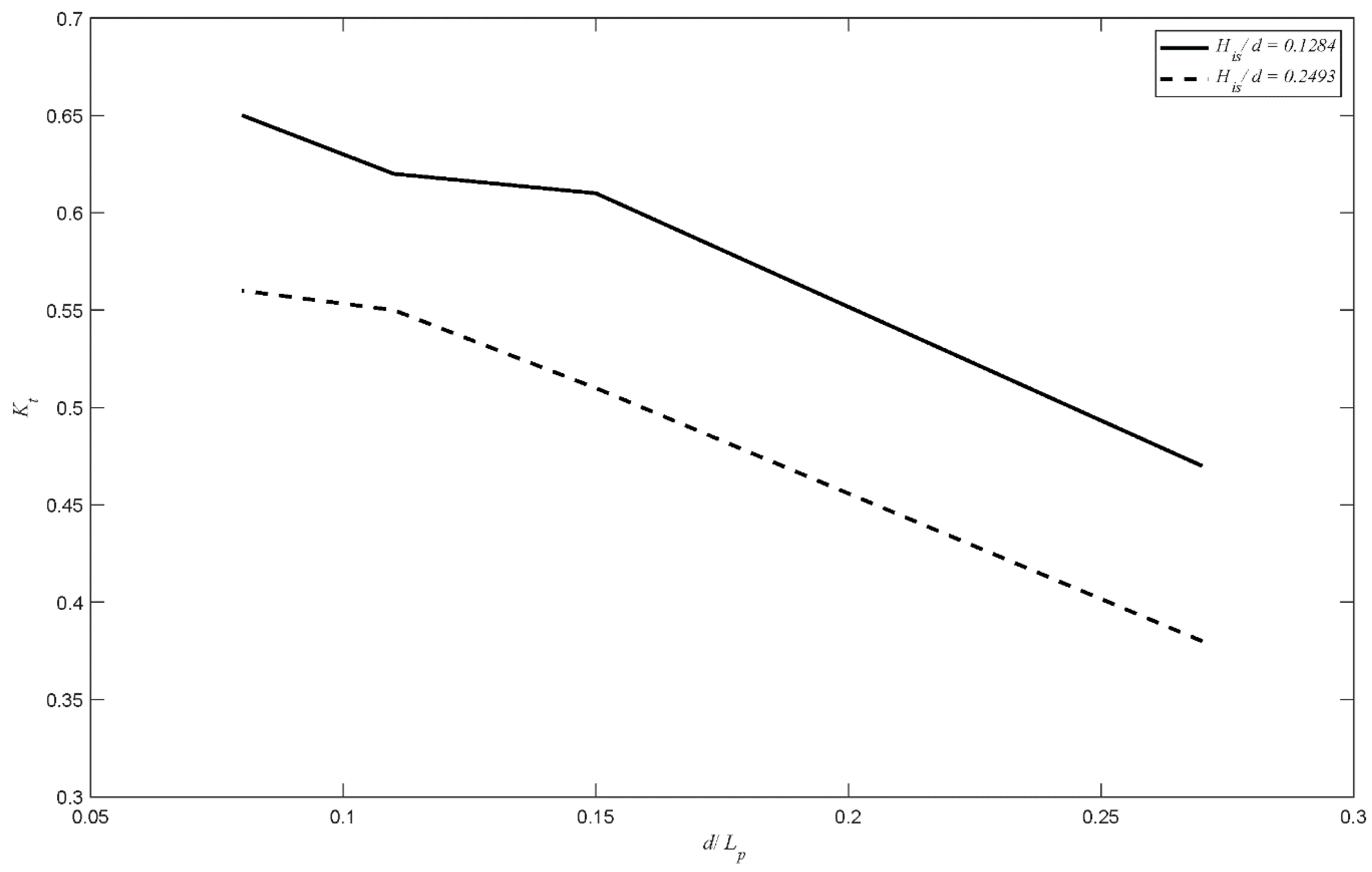
3.2.4. Effect of Relative Wave Height, His/d
3.2.5. Effect of
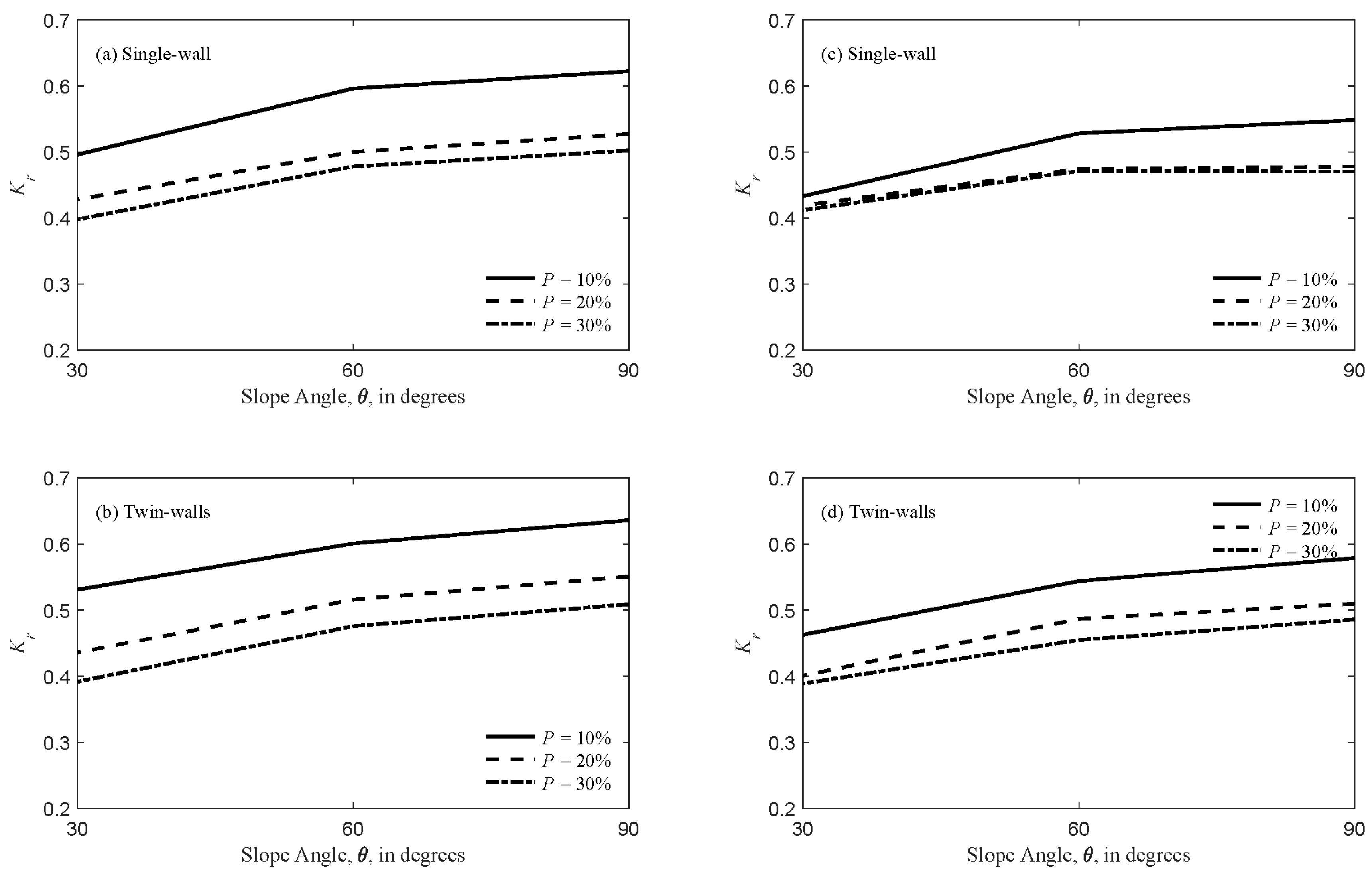
3.3. Wave Reflection Coefficient, Kr
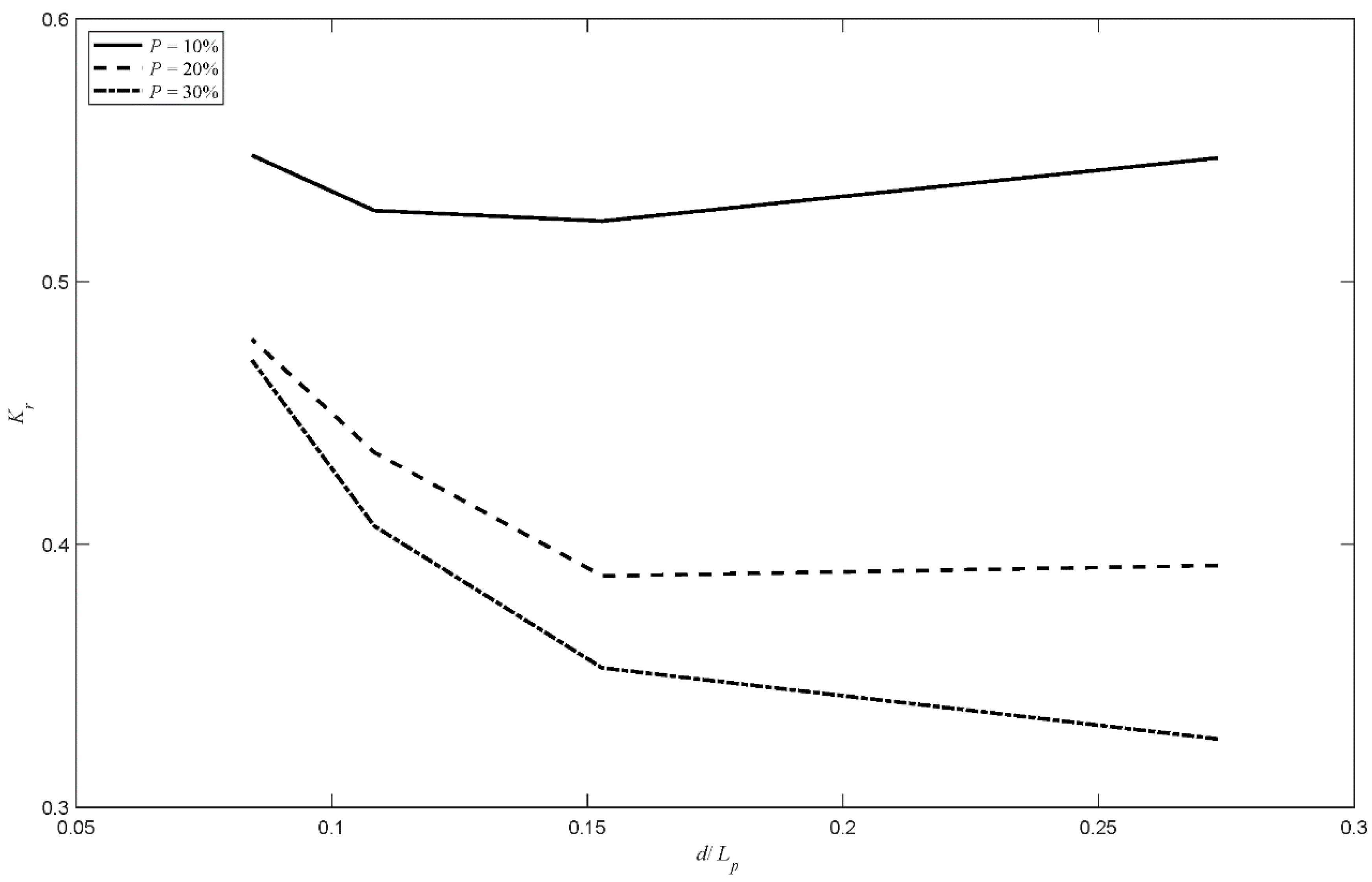
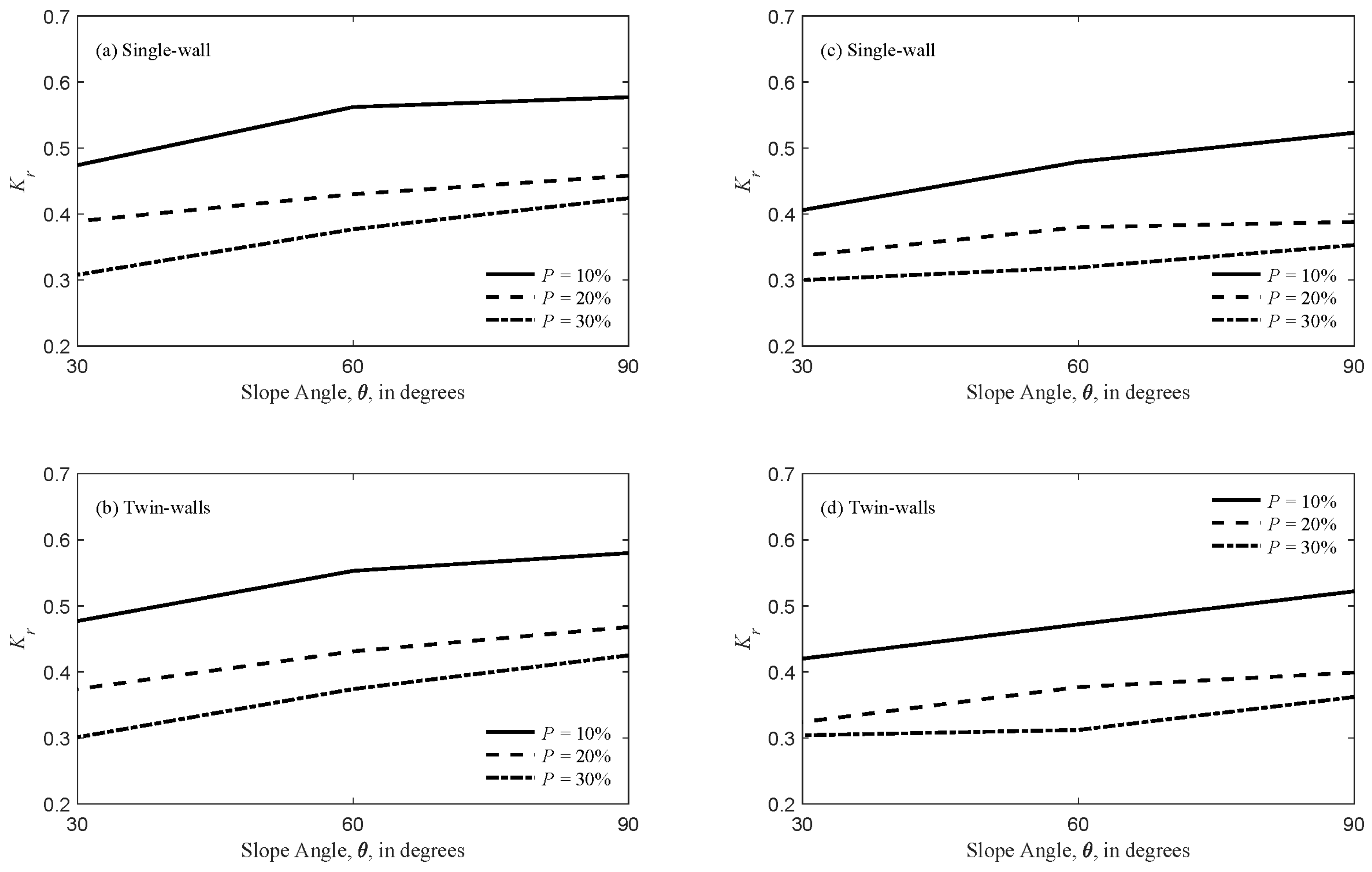
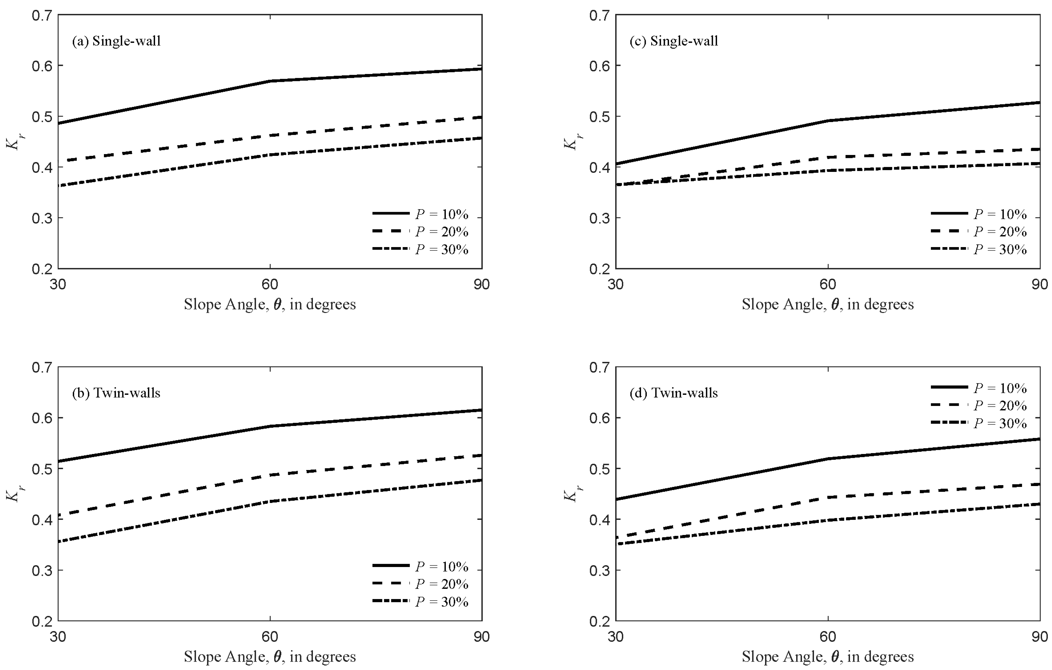
3.3.1. Effect of Porosity
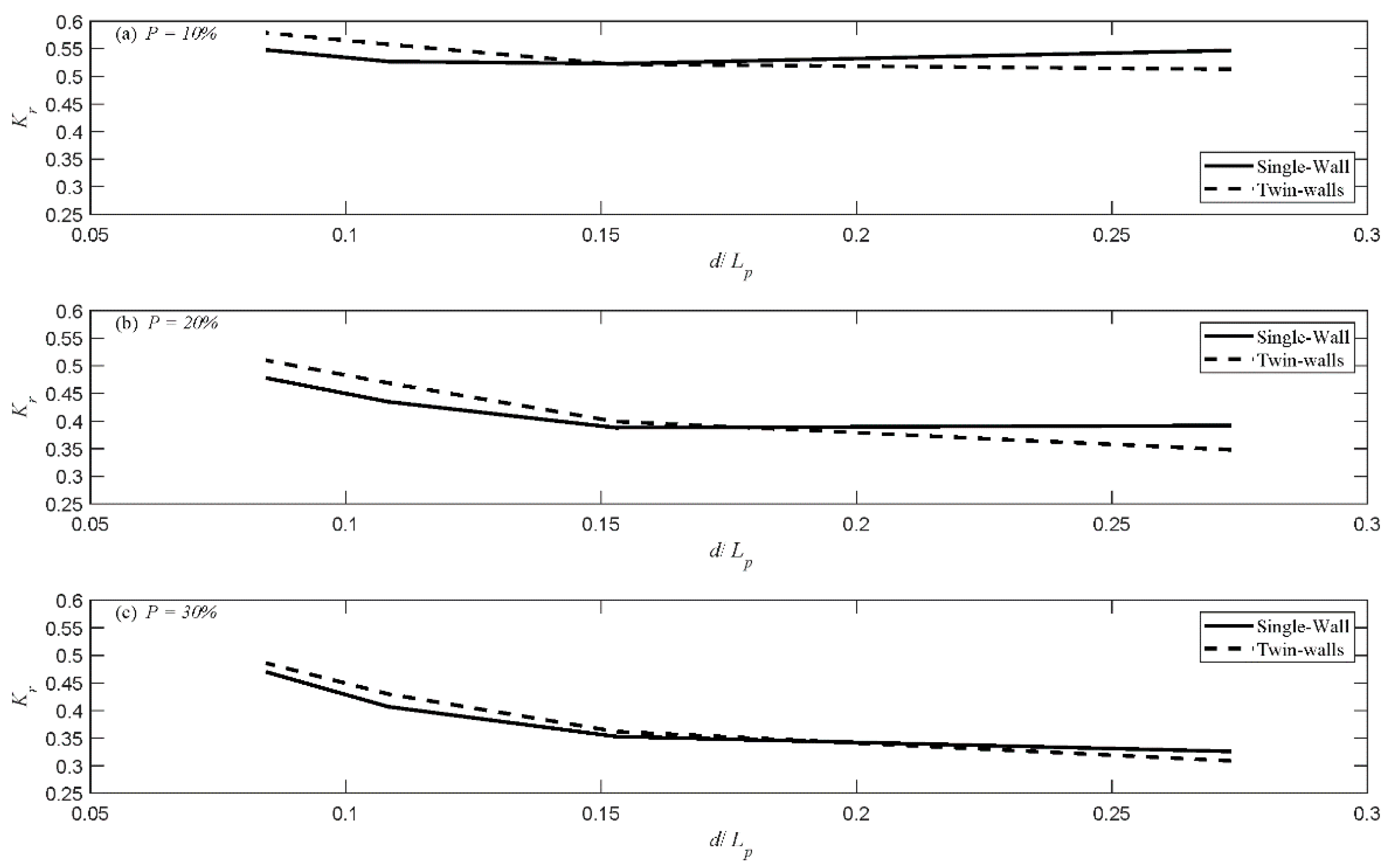
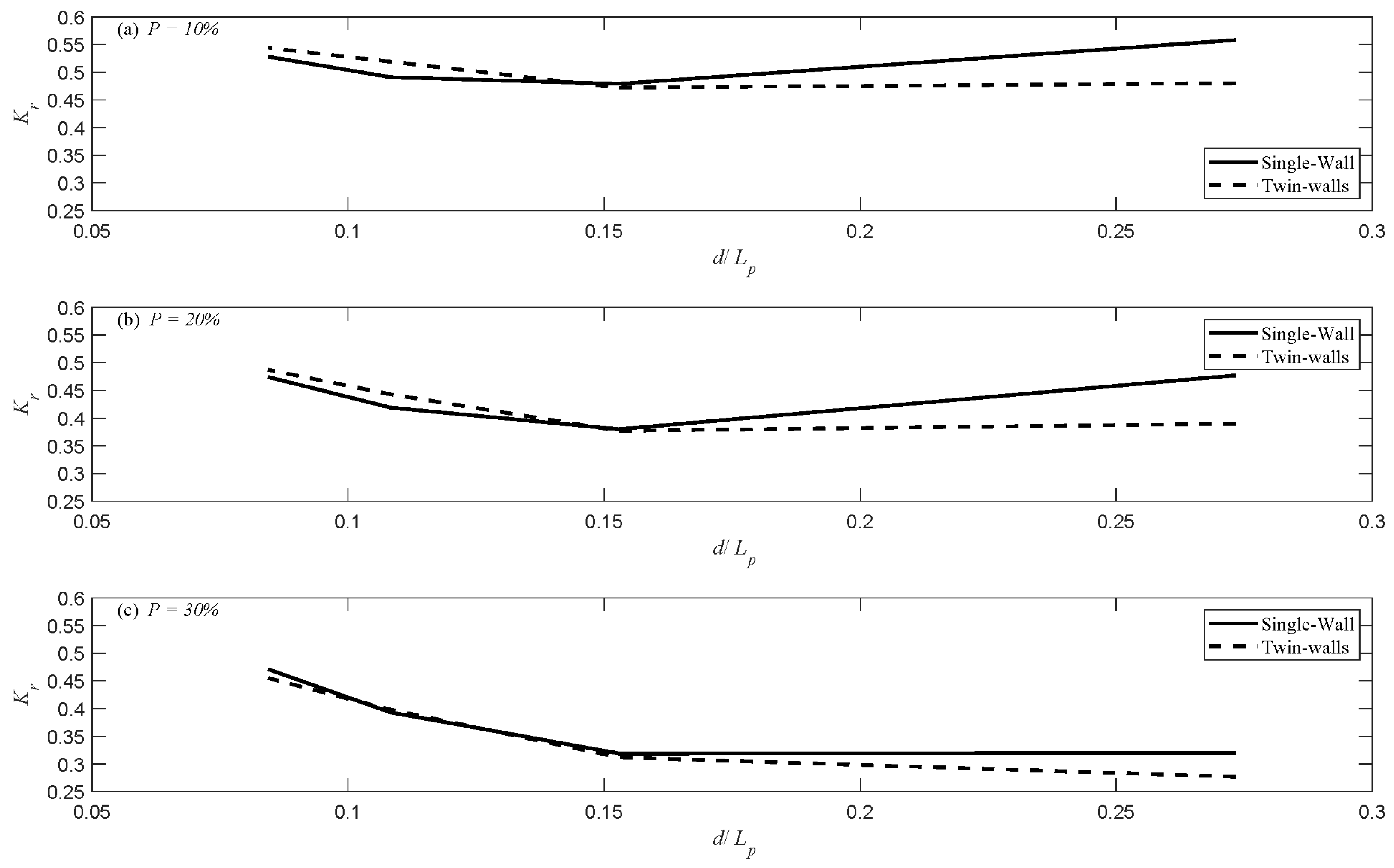
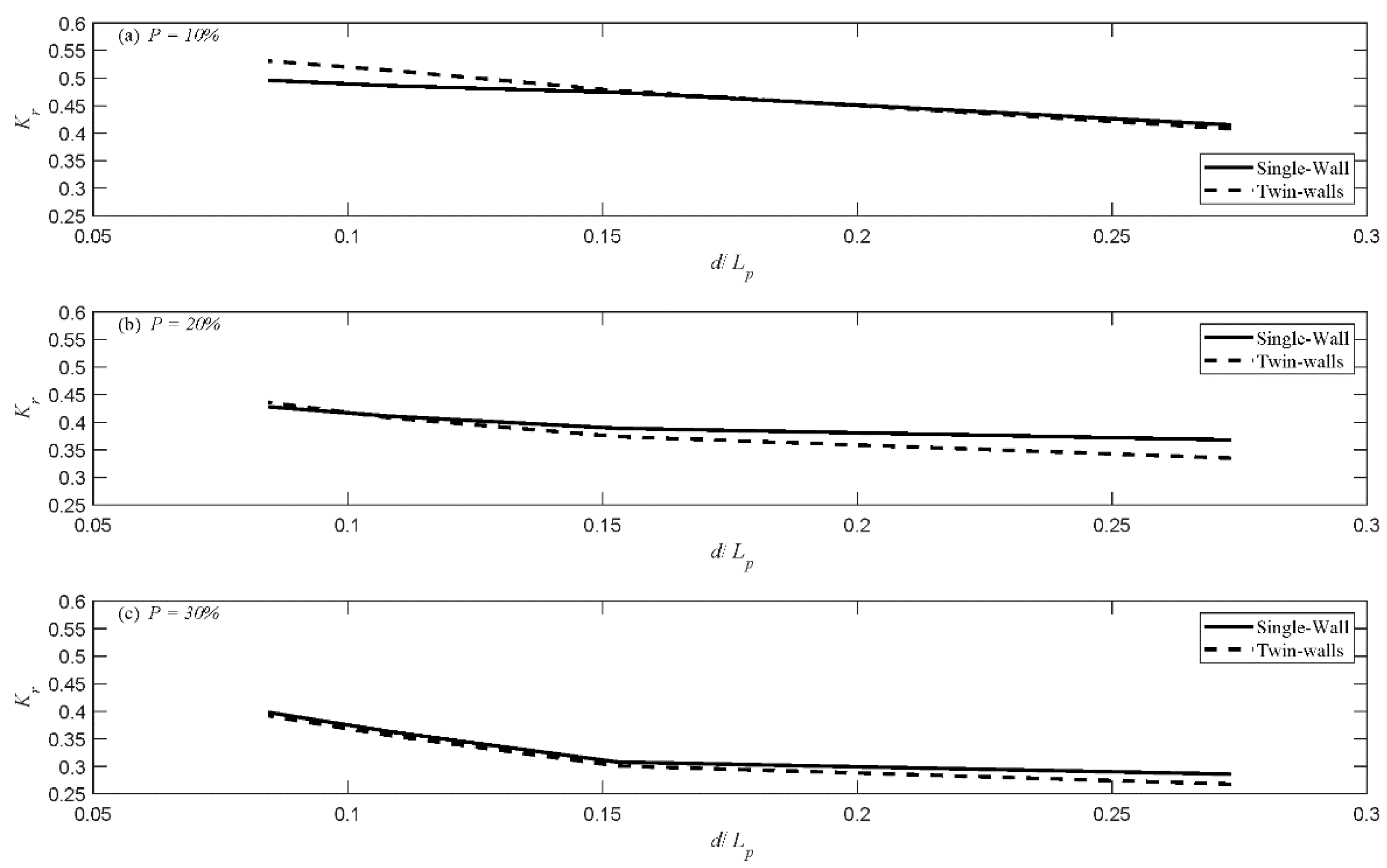
3.3.2. Effect of Number of Walls
3.3.3. Effect of Slope Angle
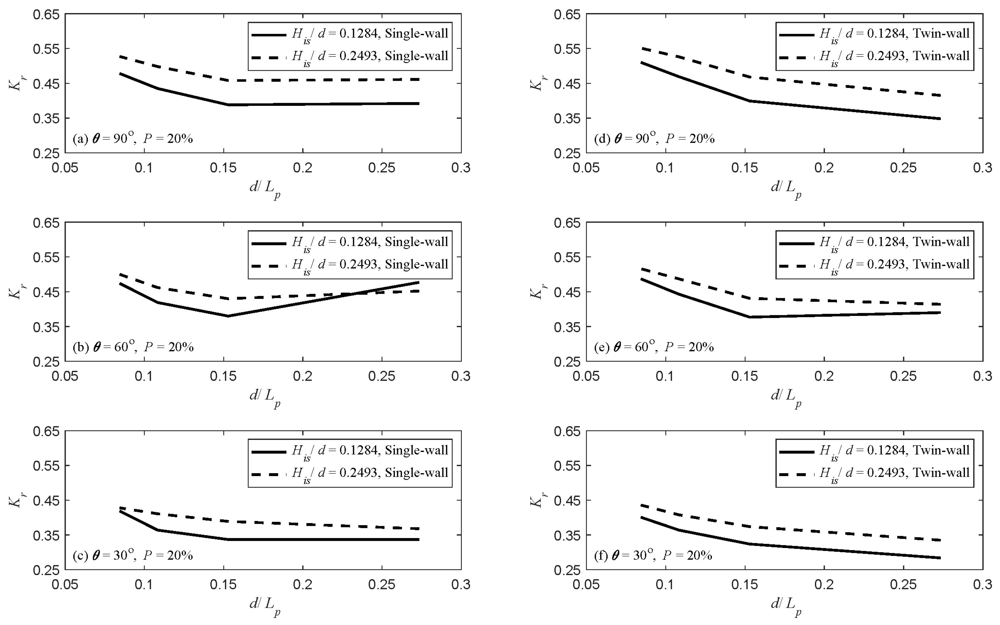
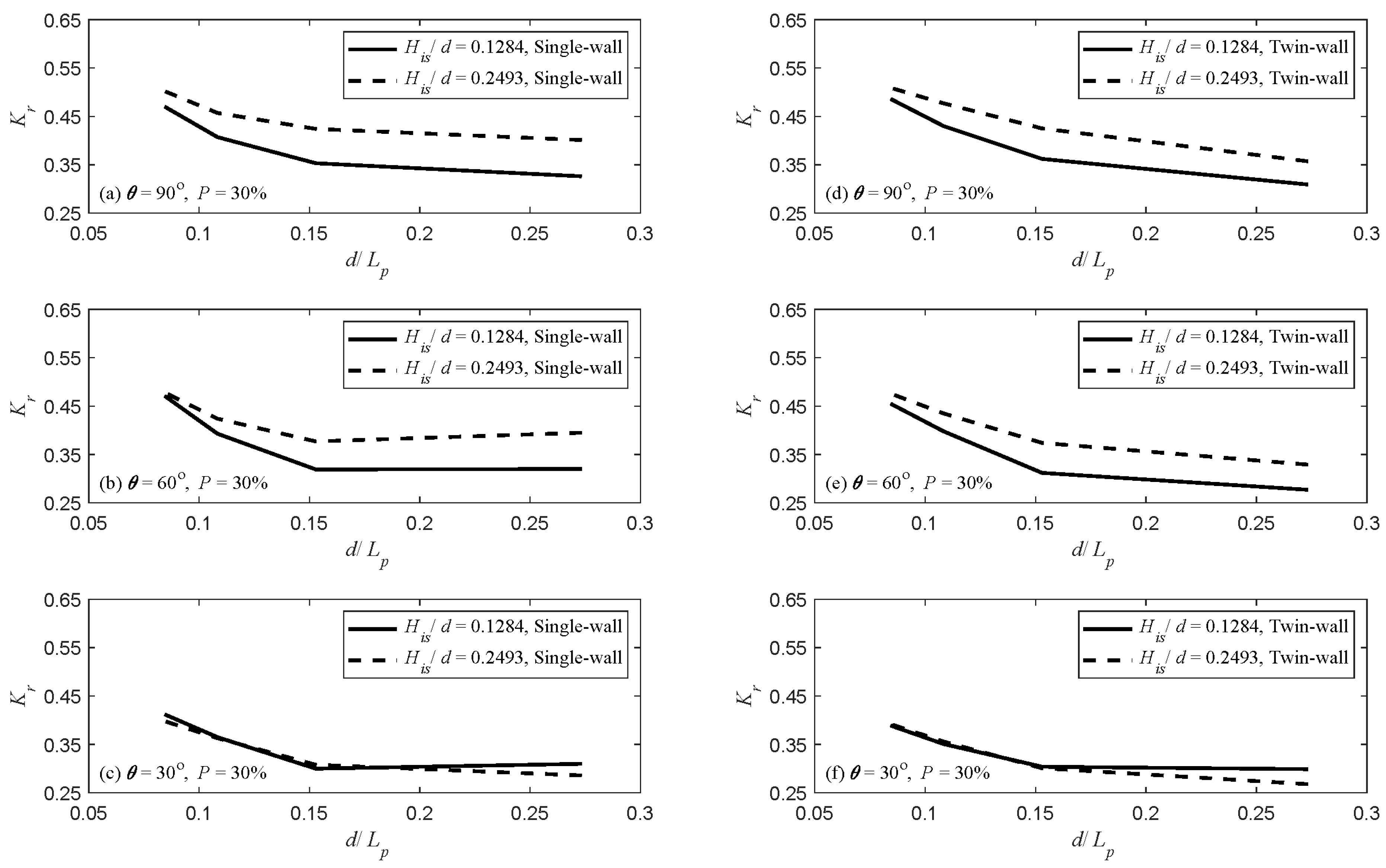
3.3.4. Effect of His/d
3.3.5. Effect of d/Lp
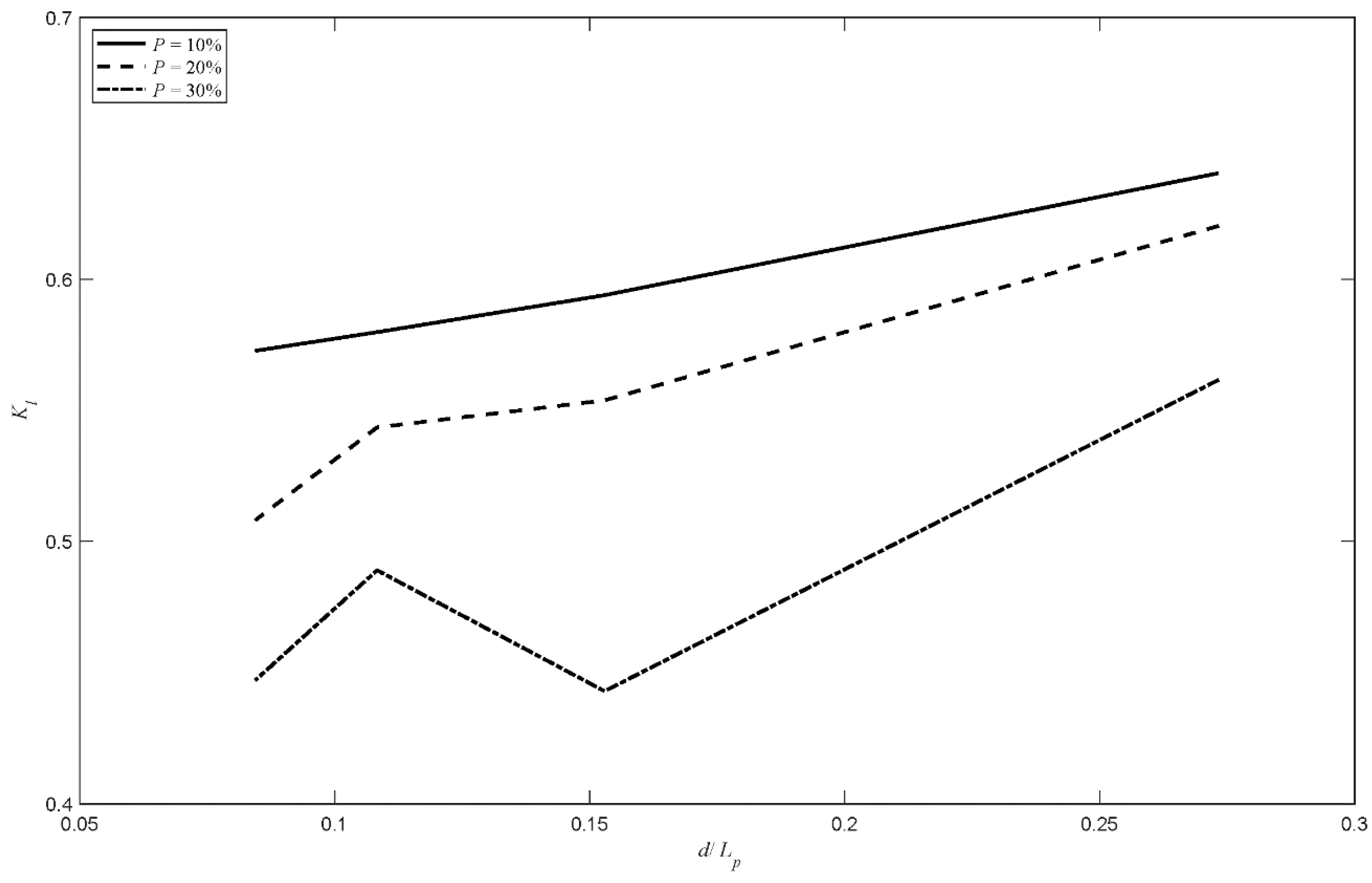
3.4. Wave Energy Dissipation Coefficient, Kl
3.4.1. Effect of Porosity
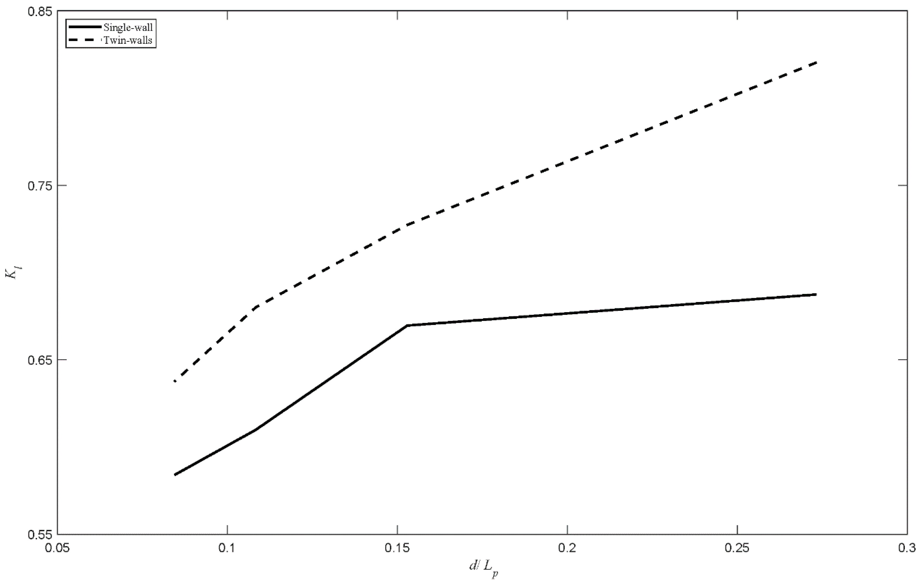
3.4.2. Effect of Number of Walls
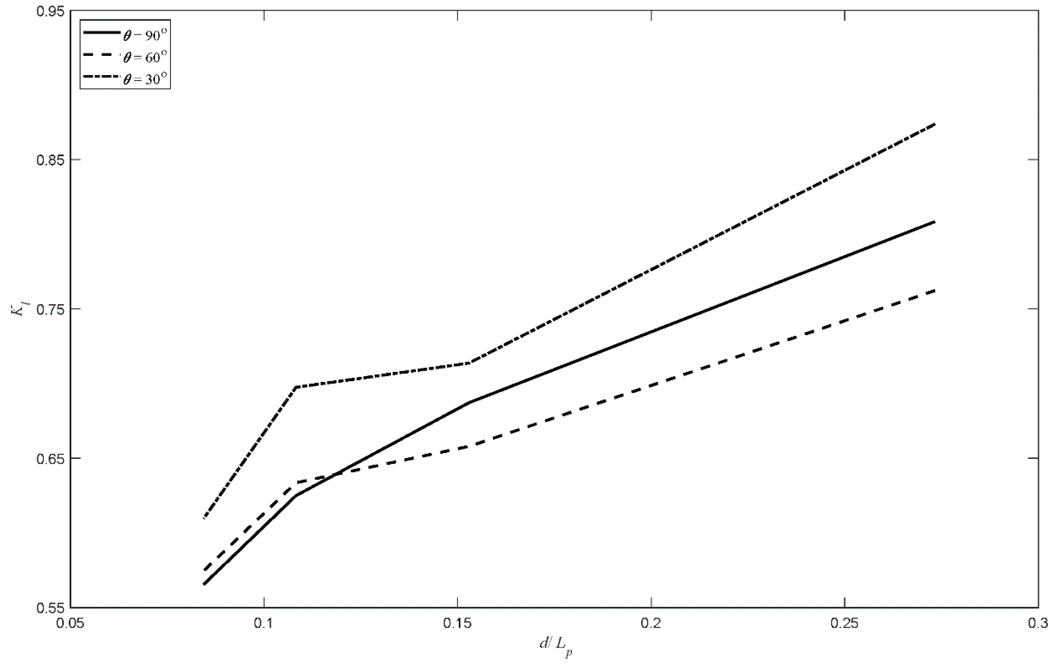
3.4.3. Effect of Slope Angle
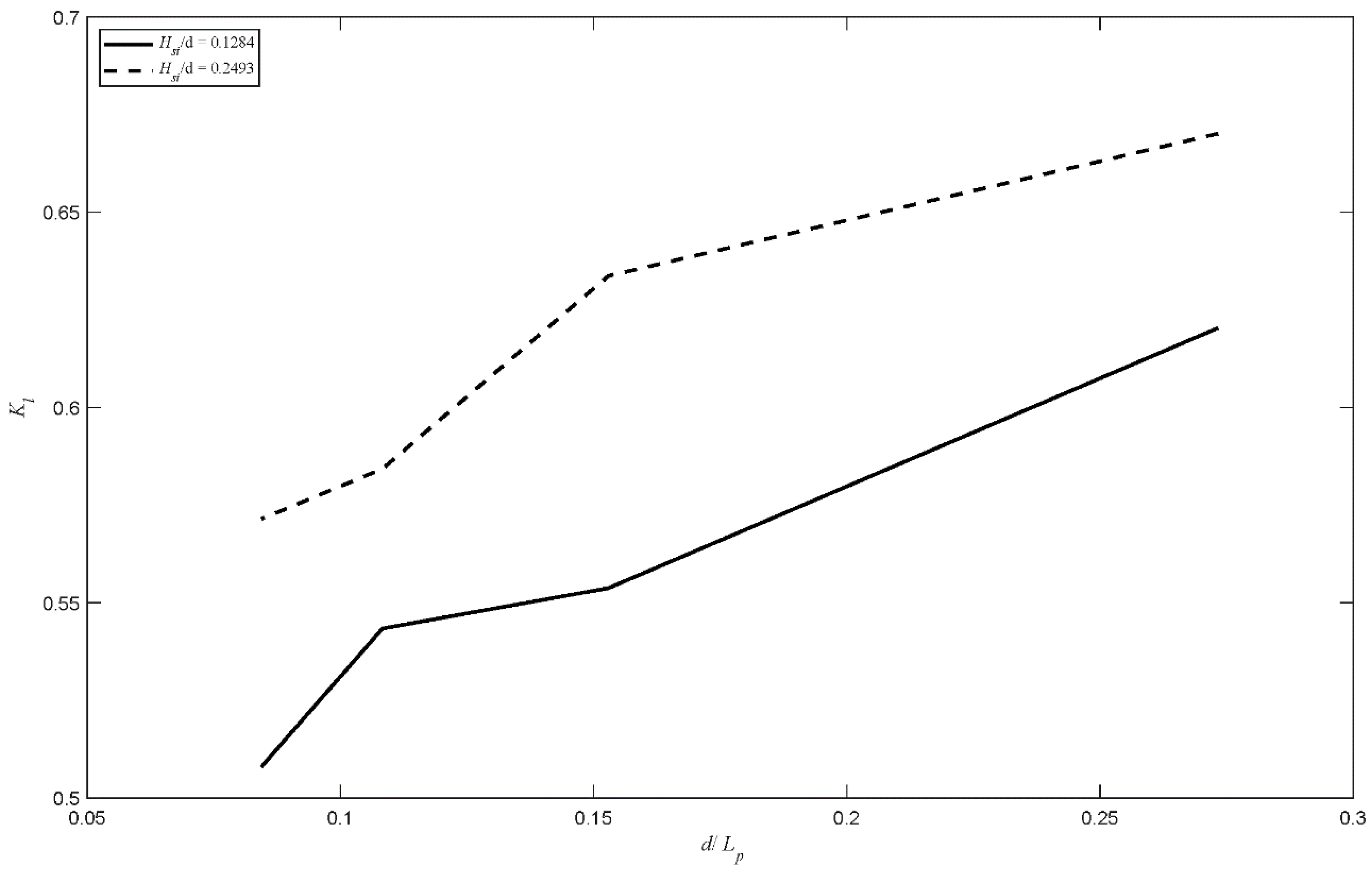
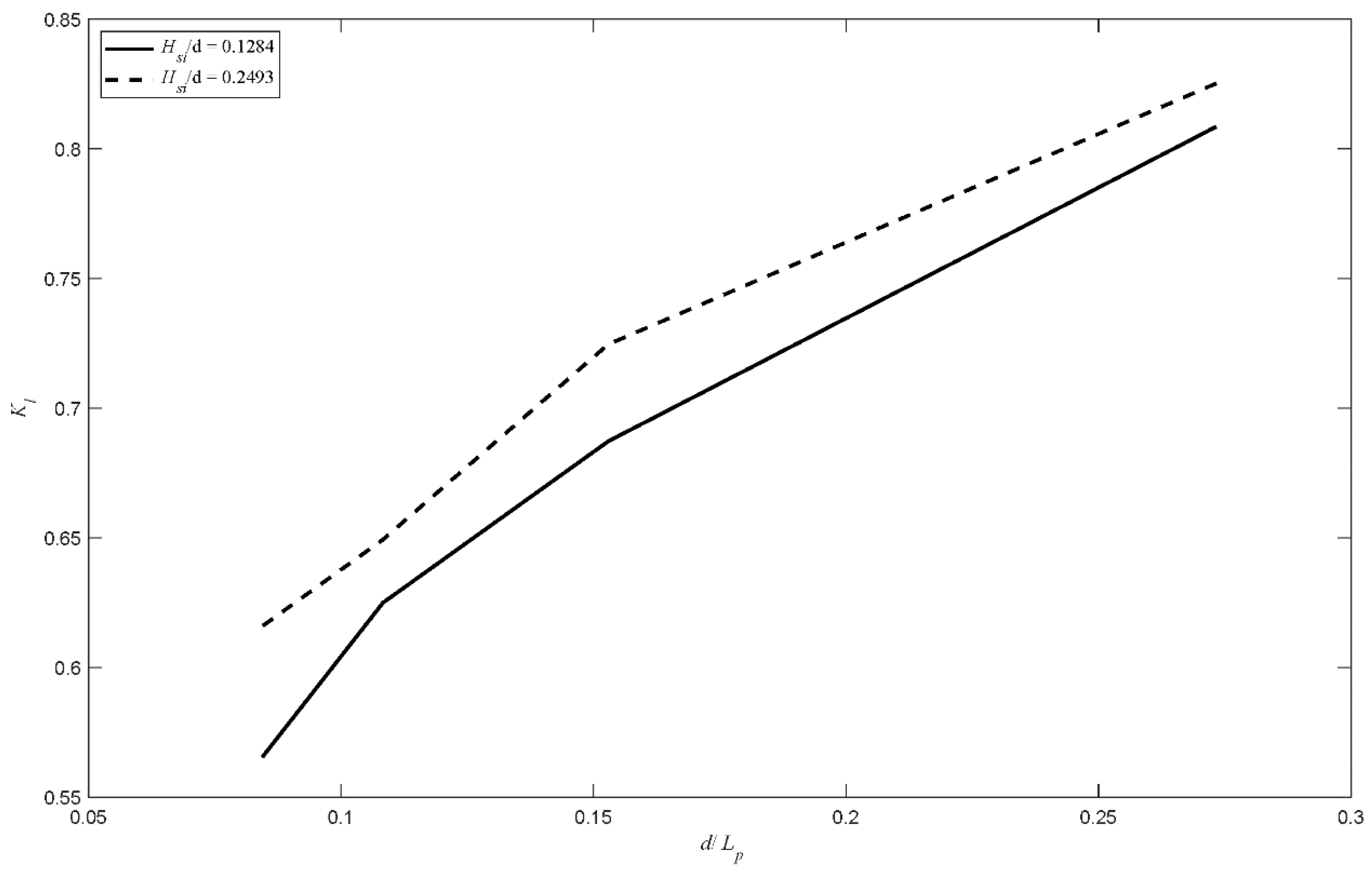
3.4.4. Effect of Relative Wave Height
3.4.5. Effect of Relative Wave Length
4. Conclusions
Author Contributions
Funding
Acknowledgments
Conflicts of Interest
References
- Sawaragi, T.; Iwata, K. Wave attenuation of a vertical breakwater with two air chambers. Coast. Eng. Jpn. 1978, 21, 63–74. [Google Scholar] [CrossRef]
- Kondo, H. Analysis of breakwaters having two porous walls. Proc. Coast. Struct. 79 1979, 2, 962–977. [Google Scholar]
- Fugazza, M.; Natale, L. Hydraulic design of perforated breakwaters. J. Waterw. Port Coast Ocean Eng. 1992, 118, 1–14. [Google Scholar] [CrossRef]
- Bergmann, H.; Oumeraci, H. Performance of New Multi Chamber Systems ys. Convention al Jarlan Caisson Breakwaters; National Civil Engineering Days-Coastal Engineering: Caen, France, 2000. [Google Scholar]
- Chen, X.; Li, Y.; Sun, D. Regular waves acting on double-layered perforated caissons. In Proceedings of the Twelfth International Offshore and Polar Engineering Conference, International Society of Offshore and Polar Engineers, Kitakyushu, Japan, 26–31 May 2002. [Google Scholar]
- Li, Y.; Liu, Y.; Teng, B. Porous effect parameter of thin permeable plates. Coast. Eng. J. 2006, 48, 309–336. [Google Scholar] [CrossRef]
- Koutandos, E.V. Hydraulic performance of double slotted barriers under regular wave attack. Wseas Trans. Fluid Mech. 2010, 5, 91–103. [Google Scholar]
- Alkhalidi, M.; Neelamani, S.; Assad, A.I.A.H. Wave forces and dynamic pressures on slotted vertical wave barriers with an impermeable wall in random wave fields. Ocean Eng. 2015, 109, 1–6. [Google Scholar] [CrossRef]
- Alkhalidi, M.; Neelamani, S.; Assad, A.I.A.H. Wave pressures and forces on slotted vertical wave barriers. Ocean Eng. 2015, 108, 578–583. [Google Scholar] [CrossRef]
- Hagiwara, K. Analysis of upright structure for wave dissipation using integral equation. In Proceedings of the 19th International Conference on Coastal Engineering, Houston, TX, USA, 3–7 September 1984; pp. 2810–2826. [Google Scholar]
- Huang, Z. Wave interaction with one or two rows of closely spaced rectangular cylinders. Ocean Eng. 2007, 34, 1584–1591. [Google Scholar] [CrossRef]
- Neelamani, S.; Al-Salem, K.; Taqi, A. Experimental investigation on wave reflection characteristics of slotted vertical barriers with an impermeable back wall in random wave fields. J. Waterw. Port Coast. Ocean Eng. 2017, 143, 06017002. [Google Scholar] [CrossRef]
- Huang, N.E.; Long, S.R. An experimental study of the surface elevation probability distribution and statistics of wind-generated waves. J. Fluid Mech. 1980, 101, 179–200. [Google Scholar] [CrossRef]
- Isaacson, M.; Baldwin, J.; Premasiri, S.; Yang, G. Wave interactions with double slotted barriers. Appl. Ocean Res. 1999, 21, 81–91. [Google Scholar] [CrossRef]
- Koraim, A.S. Hydrodynamic characteristics of slotted breakwaters under regular waves. J. Mar. Sci. Technol. 2011, 16, 331–342. [Google Scholar] [CrossRef]
- Park, W.S.; Chun, I.S.; Lee, D.S. Hydraulic experiments for the reflection characteristics of perforated breakwaters. J. Korean Soc. Coast. Ocean Eng. 1993, 5, 198–203. [Google Scholar]
- Suh, K.D.; Shin, S.; Cox, D.T. Hydrodynamic characteristics of pile-supported vertical wall breakwaters. J. Waterw. Port Coast. Ocean Eng. 2006, 132, 83–96. [Google Scholar] [CrossRef]
- Faraci, C.; Cammaroto, B.; Cavallaro, L.; Foti, E. Wave reflection generated by caissons with internal rubble mound of variable slope. Coast. Eng. Proc. 2012, 33, 51. [Google Scholar] [CrossRef]
- Neelamani, S.; Sandhya, N. Wave reflection characteristics of plane, dentated and serrated seawalls. Ocean Eng. 2003, 30, 1507–1533. [Google Scholar] [CrossRef]
- Muttray, M.; Oumeraci, H. Paper no: 247 Wave transformation at sloping perforated walls. In Solving Coastal Conundrums; Institution of Civil Engineers: London, UK, 2002. [Google Scholar]
- Mallayachari, V.; Sundar, V. Reflection characteristics of permeable seawalls. Coast. Eng. 1994, 23, 135–150. [Google Scholar] [CrossRef]
- Ahmed, H. Wave Interaction with Vertical Slotted Walls as A Permeable Breakwater; University of Wuppertal: Wuppertal, Germany, 2012. [Google Scholar]
- Mansard, E.P.; Funke, E.R. The measurement of incident and reflected spectra using a least squares method. In Proceedings of the 17th International Conference on Coastal Engineering, Sydney, Australia, 23–28 March 1980; pp. 154–172. [Google Scholar]
- Goda, Y.; Suzuki, Y. Estimation of incident and reflected waves in random wave experiments. In Proceedings of the 15th International Conference on Coastal Engineering, Honolulu, HI, USA, 11–17 July 1976; pp. 828–845. [Google Scholar]


| Wall Parameter | Notation | Range Tested |
|---|---|---|
| Porosity | P | 10%, 20%, and 30% |
| Number of walls | N | 1 and 2 |
| Slope angle | θ | 30, 60, and 90 |
| Parameter | Description | Range |
|---|---|---|
| His/d | Relative wave height | 0.1284–0.2493 |
| d/Lp | Relative wave period | 0.0844–0.2733 |
| His/Lp | Wave steepness | 0.0106–0.0683 |
| Coefficient | Highest Value | Corresponding Model | Lowest Value | Corresponding Model |
|---|---|---|---|---|
| Kt | 0.824 | N = 1, P = 30%, θ = 90 | 0.314 | N = 2, P = 10%, θ = 30 |
| Kr | 0.636 | N = 2, P = 10%, θ = 90 | 0.268 | N = 2, P = 30%, θ = 30 |
| Kl | 0.889 | N = 2, P = 20%, θ = 30 | 0.418 | N = 1, P = 30%, θ = 60 |
| θ Change: | 90–60 | 90–30 | 60–30 | 90–60 | 90–30 | 60–30 |
|---|---|---|---|---|---|---|
| Statistical Parameter | Single Wall | Twin Walls | ||||
| Mean | 4.21 | 4.56 | 3.87 | 3.45 | 4.11 | 3.21 |
| Standard Deviation | 3.47 | 2.73 | 1.69 | 2.50 | 3.58 | 1.39 |
| Minimum | 0.24 | 0.64 | 1.25 | 0.41 | 0.52 | 1.30 |
| Maximum | 10.16 | 10.39 | 6.78 | 8.84 | 10.44 | 4.89 |
| θ Change: | 90–60 | 90–30 | 60–30 | 90–60 | 90–30 | 60–30 |
|---|---|---|---|---|---|---|
| Statistical Parameter | Single Wall | Twin Walls | ||||
| Mean | 1.37 | 11.42 | 8.12 | 4.37 | 11.08 | 8.60 |
| Standard Deviation | 1.17 | 6.63 | 6.31 | 5.03 | 8.96 | 7.37 |
| Minimum | 0.03 | 0.41 | 0.03 | 0.21 | 0.40 | 0.98 |
| Maximum | 2.92 | 20.22 | 17.82 | 14.18 | 24.79 | 23.58 |
| S | P% | His/d | Maximum% of Kr Decrease | Maximum% of Kr Increase | Average% of Kr Change |
|---|---|---|---|---|---|
| 90° | 10 | 0.1284 | 5.88 | 6.22 | −1.28 |
| 60° | 10 | 0.1284 | 5.70 | 13.98 | 1.68 |
| 30° | 10 | 0.2493 | 7.06 | 1.69 | −2.94 |
| 90° | 20 | 0.1284 | 7.82 | 11.22 | −1.53 |
| 60° | 20 | 0.1284 | 5.73 | 18.24 | 2.64 |
| 30° | 20 | 0.2493 | 1.87 | 8.97 | 2.92 |
| 90° | 30 | 0.1284 | 5.65 | 5.21 | −1.60 |
| 60° | 30 | 0.1284 | 1.27 | 13.44 | 4.44 |
| 30° | 30 | 0.2493 | - | 6.29 | 3.00 |
© 2020 by the authors. Licensee MDPI, Basel, Switzerland. This article is an open access article distributed under the terms and conditions of the Creative Commons Attribution (CC BY) license (http://creativecommons.org/licenses/by/4.0/).
Share and Cite
Alkhalidi, M.; Alanjari, N.; Neelamani, S. Wave Interaction with Single and Twin Vertical and Sloped Slotted Walls. J. Mar. Sci. Eng. 2020, 8, 589. https://doi.org/10.3390/jmse8080589
Alkhalidi M, Alanjari N, Neelamani S. Wave Interaction with Single and Twin Vertical and Sloped Slotted Walls. Journal of Marine Science and Engineering. 2020; 8(8):589. https://doi.org/10.3390/jmse8080589
Chicago/Turabian StyleAlkhalidi, Mohamad, Noor Alanjari, and S. Neelamani. 2020. "Wave Interaction with Single and Twin Vertical and Sloped Slotted Walls" Journal of Marine Science and Engineering 8, no. 8: 589. https://doi.org/10.3390/jmse8080589
APA StyleAlkhalidi, M., Alanjari, N., & Neelamani, S. (2020). Wave Interaction with Single and Twin Vertical and Sloped Slotted Walls. Journal of Marine Science and Engineering, 8(8), 589. https://doi.org/10.3390/jmse8080589