5.2. System Parametrization
The SSS data has been processed as described in
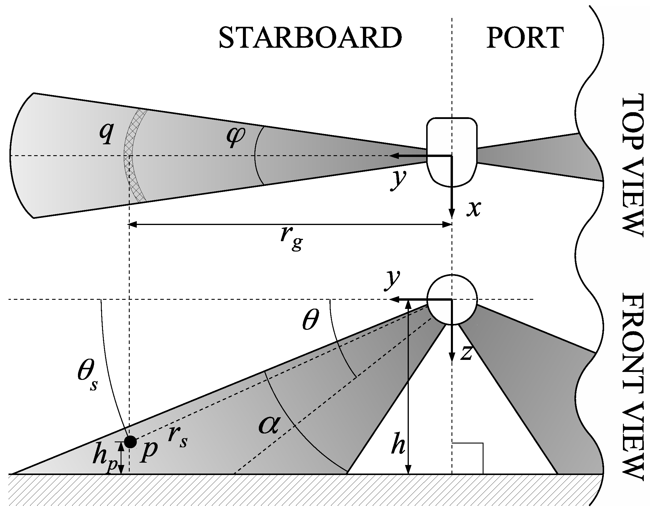
Section 3. To this end, the ensonification pattern, modelled by Equation (
5), has been computed for each emitted ping and, thus, for each gathered swath using the parametrization shown in
Table 1.
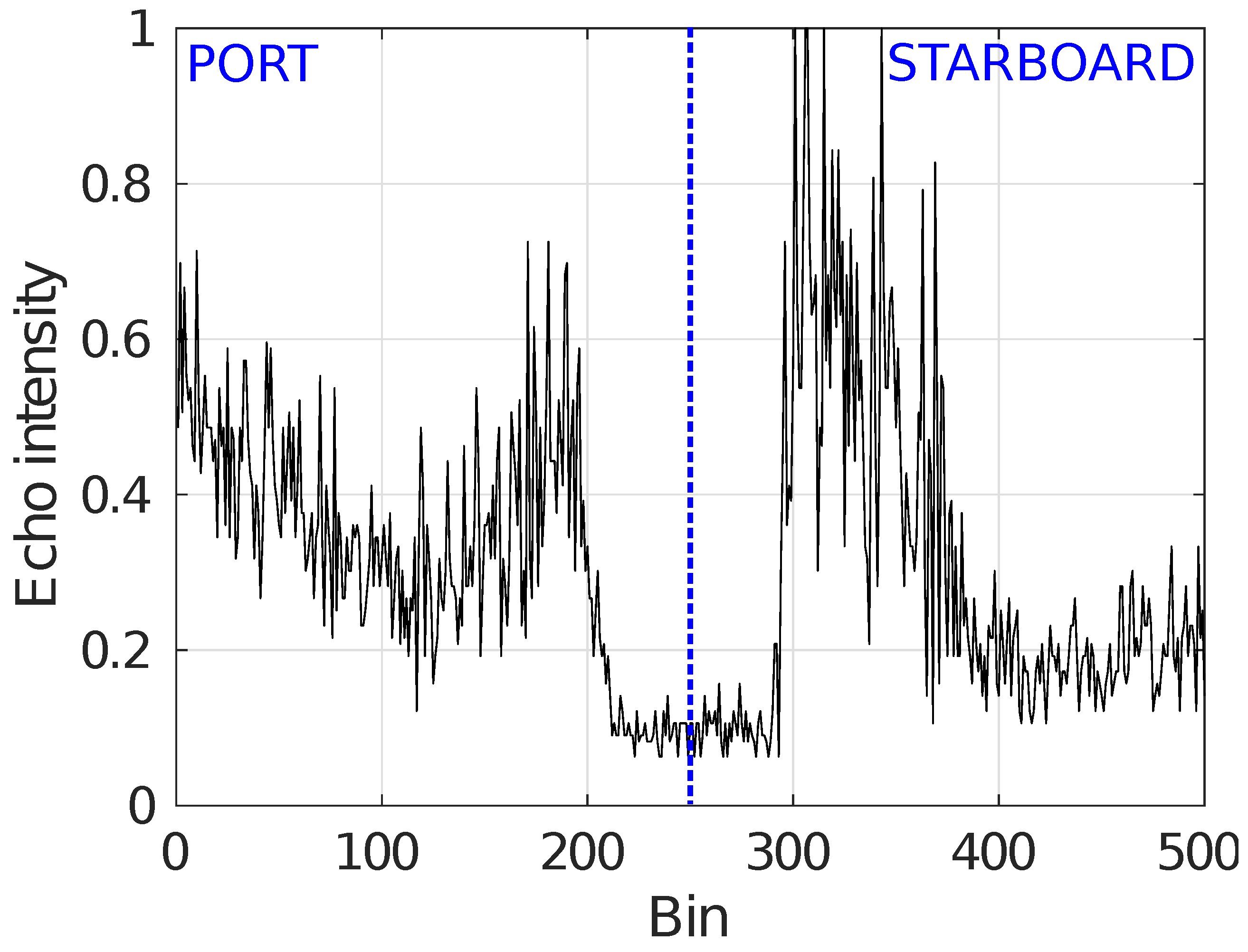
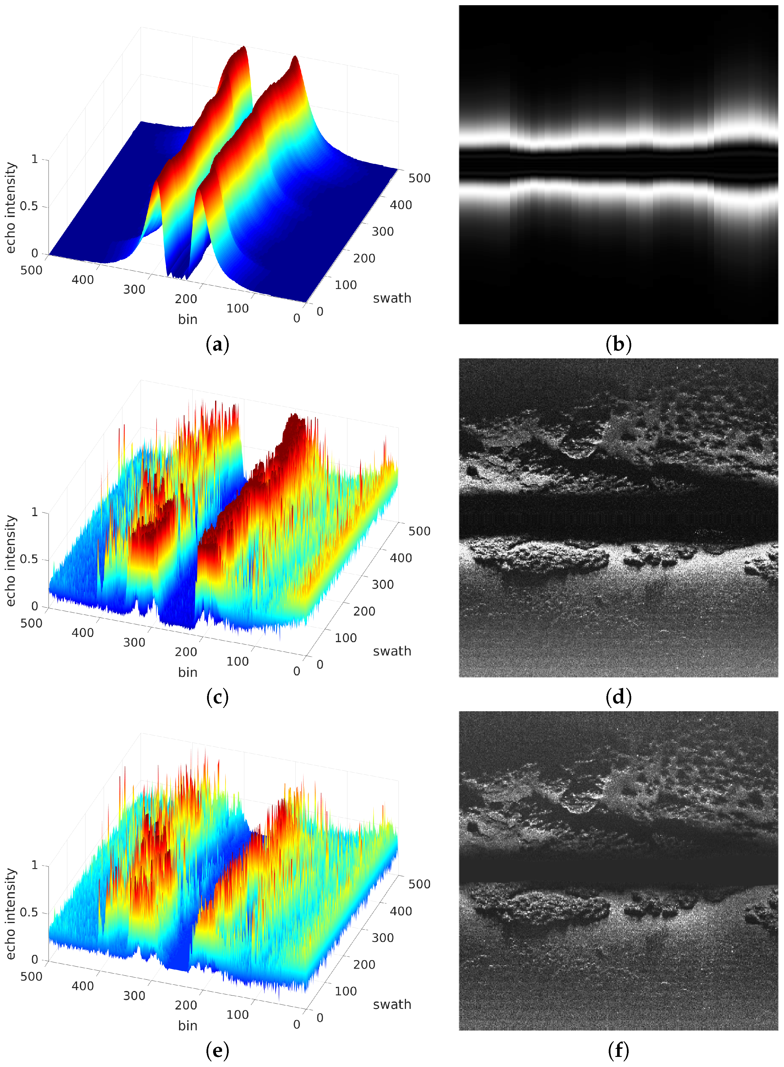
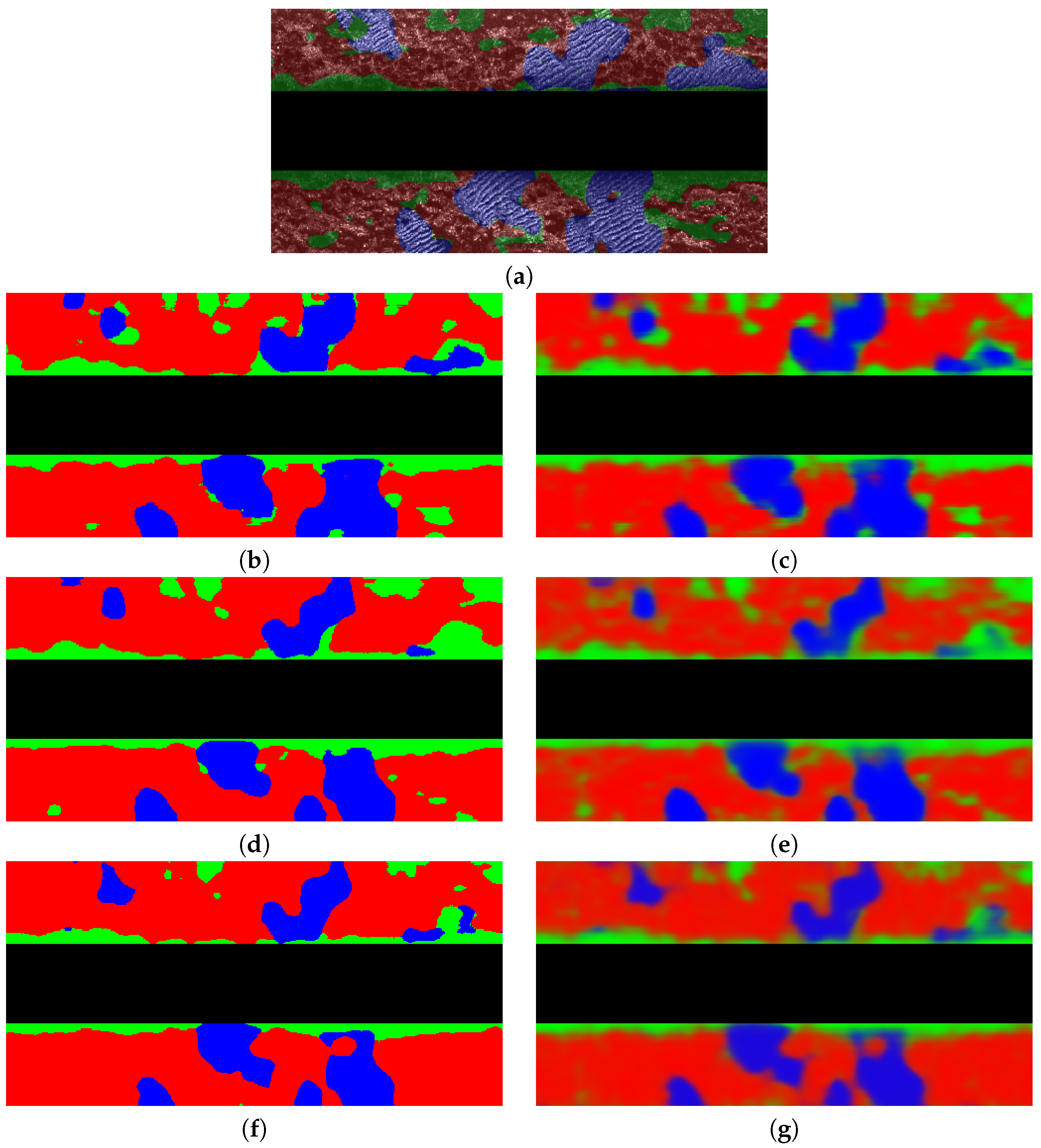
Figure 11a depicts the obtained values along a short transect. Changes along track are due to changes in altitude. As it can be observed, the ensonification pattern clearly reflects the two sensing heads and the blind zone. It also illustrates the two peaks showing the parts of the ER that will be ensonified with more energy.
Figure 11b shows the same values in a 2D plane where the color intensity illustrates the ensonification intensity.
Figure 11c shows the SSS data gathered along the same short transect used to build the ensonification pattern. As it can be observed, the regions close to the blind zone are responsible for very large echo intensities, reaching a condition close to saturation and making it difficult to distinguish objects within these regions. This effect can be also observed in
Figure 11d, which shows the same data in the bin-swath plane using color intensity to represent the echo intensity.
The ensonification pattern is used to correct the raw SSS data. Thanks to that, the echo intensity is homogenized, desaturating the regions close to the blind zone and thus emphasizing the existing objects in the acoustic image.
Figure 11e shows the result of applying the ensonification pattern to the raw SSS data using Equation (
10) and performing the slant range correction by means of Equation (
11). The same data projected to a 2D plane is depicted in
Figure 11f.
As it can be observed, the objects close to the blind zone are more distinguishable from the background that in the original data, revealing some small details that were not appreciable in the raw SSS swaths. This process can be seen as a physics based contrast enhancement that leads to an homogeneous contrast almost independently of the bin location, thus helping the operation of segmentation algorithms.
By observing the examples in
Figure 11 it can be seen not only the blind zone but also that, from a certain bin onward, both on port and on starboard, the echo intensity is so small that is is difficult to clearly ascertain the structure of the ocean floor, even in the intensity corrected version. This is particularly clear in the starboard part of
Figure 11d,f. These are, precisely, the low contrast zones mentioned in
Section 3.4.
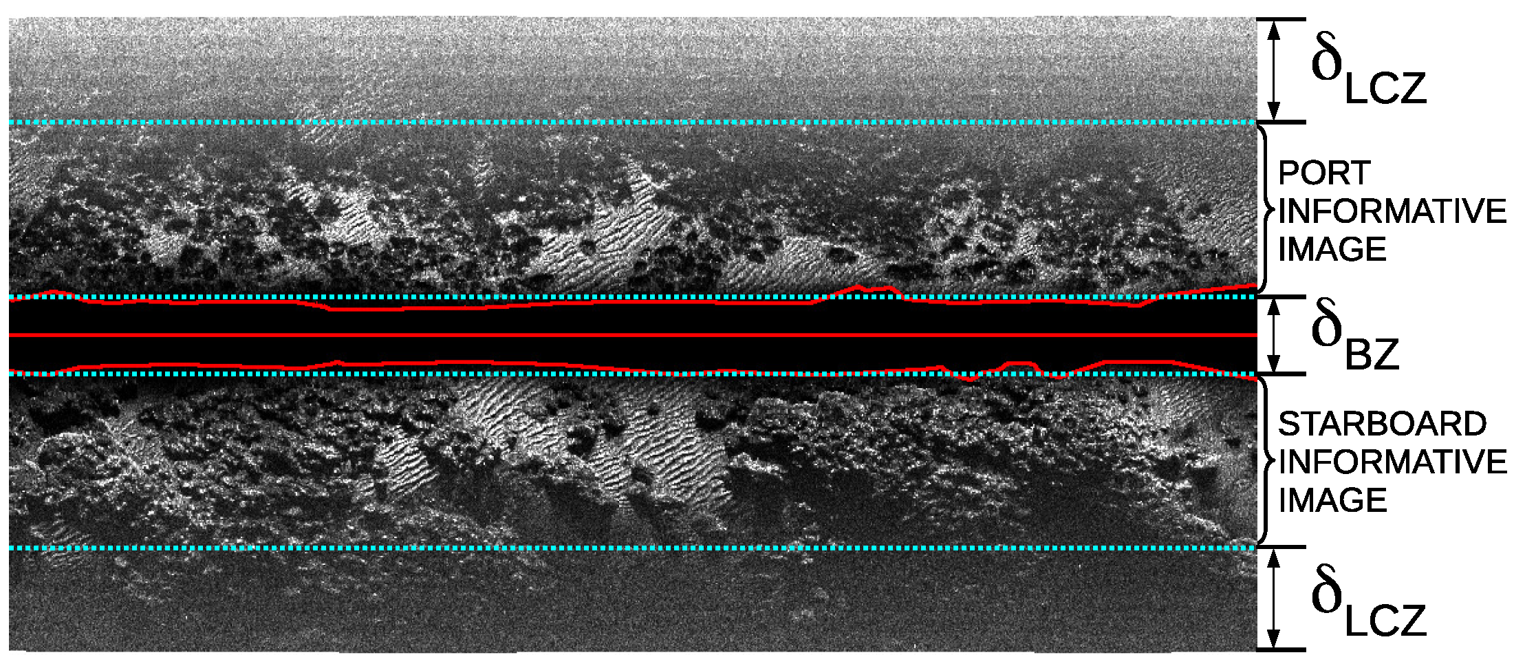
As mentioned in that section, to reduce the problems that the non informative blind and low contrast zones would induce in the subsequent segmentation, they are removed. To this end, the parameters and have been defined. In order to determine these parameters, we proceeded as follows.
First, we computed the average FBR using Equation (
4), the average AUV altitude and performing the flat floor assumption. This obtained average FBR is 25 bins (both on port and starboard) and is directly related to
. As a matter of fact, according to
Figure 4,
should twice the FBR. Thus, we determined in this way that
.
Since the low contrast zone is mainly due to the low ensonification intensity for large distances, we used Equation (
5) to determine
. More specifically, given that
, we have searched the
that keeps the 90% of the ensonification intensity within each informative image. By using this procedure, we have found that
.
Taking into account that the SSS used in the experiments provides 250 bins per sensing head, this means that each informative image, as defined in
Section 3.4 and illustrated in
Figure 4, is composed of 83 bins. This an approximation based on the assumption of a flat floor and a constant navigation altitude. Even though computing
and
on-line using instantaneous altitude measurements may seem a better option, that approach would lead to changes in size of the informative image which would be problematic in further segmentation steps. That is why this study uses the constant
and
approximation.
Finally, the value of the patch margin
, presented in
Section 4.2.1, has been set to
so that the number of swaths in patch, which is
, equals the number of bins, which is 83. Thanks to this, the NN will be fed with square patches.
5.3. Quantitative Results
After tuning
,
and
we conducted some experiments to quantitatively evaluate our proposal and the effect of
and
. As explained in
Section 4.2.1, the patch separation
defines the number of swaths between the centers of the patches used to feed the NN during training. In this way, a value of
means that a sliding window over the whole informative images is used to train the system and
uses strictly non overlapping patches to train the NN. Values larger than
N are not considered since that means that some input data is discarded.
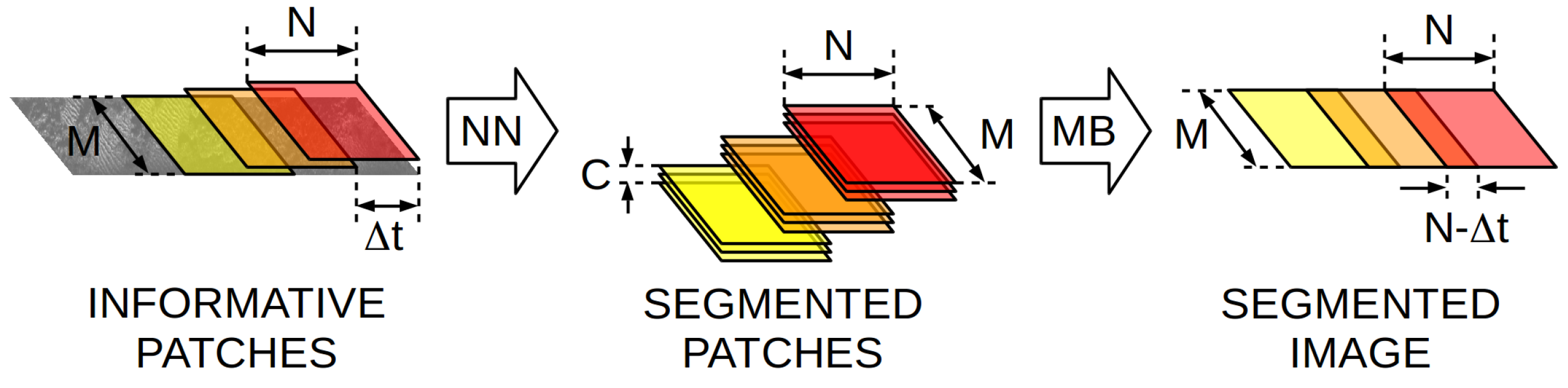
Figure 6 illustrates the meaning of
. Independently of the value of
, the order in which the patches are used to feed the NN is randomized in order to prevent overfitting.
The meaning of
, which also lies in the interval [1,N], is similar to the one of
but it refers to the separation between patches during the on-line usage of the NN. Its was explained in
Section 4.2.2.
The tested values of are 1, and N. The tested values for are also 1, and N. In this way, we explore the effects of using small, medium and large values for both parameters. Given that in our case , this means that the explored values are 1, 41 and 83. Both the single class (SCM) and the multi class (MCM) methods have been evaluated using all the combinations of parameters mentioned before. This leads to eighteen tested configurations, nine being for SCM and nine for MCM.
For each of the mentioned eighteen combinations, a K-Fold cross validation with has been performed. To evaluate the quality, the resulting segmented image has been compared to the ground truth and the confusion matrix has been constructed. In the case of MCM, the most probable class for each bin in the resulting segmented image has been used to do the comparison.
Let the components of the confusion matrix be named , so that denotes the number of bins predicted to be of class x that actually are of class y, where x and y can be 0, 1 or 2, denoting the classes rock, sand and others respectively. Thus, the correct classifications are those where .
It is important to emphasize that the decision of a classification being correct or not is performed by comparing the classification itself to a hand labelled ground truth. This ground truth is, by definition, imperfect since it can be subject to human interpretation. Also, some regions may be difficult to classify even for a human, especially in the boundaries between classes and some subjective decisions have to be made in these cases. Thus, the presented results can be slightly influenced by these imperfections in the ground truth.
Confusion matrices are a useful tool to quantify and visualize how the segmentation errors are distributed among classes and what classes are more likely to be wrongly classified as another one. In order to provide a clear representation, these matrices are often normalized according to two methods. It is important to emphasize that these methods actually provide the same information but from a different point of view.
The first method is the column-wise normalization, which scales the columns down to sum one. Since columns depict the true classes, column-wise normalization means that the value in row r and column c represents the ratio of bins whose true class is c that have been classified as class r. Thus, this kind of normalization emphasizes the distribution of classes in which the bins of a specific class have been classified.
The second method is the row-wise normalization. In this case, the rows are scaled down to sum one. Rows representing the predicted classes, this format means that the value in row r and column c represents the ratio of bins classified as class r that actually are of class c. Thus, this normalization approach shows the ratio of each of the true classes given the bins predicted to belong to one specific class.
More specifically,
Table 3a shows the confusion matrix corresponding to all the configurations of
and
using SCM and normalized column-wise. It can be observed how the largest values appear in the diagonal, meaning that the ratio of bins correctly identified is the largest one. It can also be observed how classes are confused among themselves. For example, the matrix shows that the 16.25% and the 4.57% of the rocks have been classified as sand and other respectively, thus emphasizing that rocks are misclassified as sand about four times more than they are confused with other.
Table 3b shows the SCM row-wise normalized confusion matrix. It can be observed, for example, that the 88.03% of the bins classified as rock were actually rocks and that the 10.22% and the 1.74% were actually sand and other respectively. Thus, given one bin wrongly classified as rock it is about ten times more likely that it actually is sand than other.
Table 4a,b show the MCM confusion matrices normalized column-wise and row-wise respectively. By comparing them to their SCM counterparts it can be observed that the differences are really small, though suggesting that only minor improvements arise from the use of MCM.
Using the raw confusion matrices, different quality indicators have been computed. The first one is the accuracy
A, defined as the ratio of correctly classified bins with respect to the total number of bins being classified:
The obtained results for SCM and MCM are shown in
Table 5. There are no significant differences between the single class and the multi class approaches, independently of the values of
and
.
Also, it can be observed how, overall, the accuracy decreases as the value of or increases. In all cases, however, the accuracy is really high, ranging between an 87.7% in the worst case (SCM, and ) to a 91.0% in the best case (SCM and MCM, ).
The results also show that has less influence in the resulting accuracy that . This fact is particularly interesting because small values of or lead to larger computational requirements, as it will be shown later. Since is only used during training, a small value of will not influence the on-line usage of our system and a large value could be used for , allowing a fast segmentation without compromising the quality.
Since our proposal is multi-class, let us evaluate its performance for each of the three proposed classes. To this end, the multi-class versions of the precision, recall, fall-out and F1-score indicators will be used.
The precision
of the class
i is defined as the ratio between the number of bins correctly classified as being of class
i and the total number of bins classified as class
i, both correct and incorrect:
The recall
, also known as sensitivity, of the class
i is the ratio between the number of bins correctly classified as being of class
i with respect to the total number of bins that actually are of class
i, independently of how they have been classified:
The fall-out
of class
i is the ratio between the number of bins incorrectly classified as being of class
i and the number the number of bins which are not of class
i independently of how they have been classified.
Finally, the F1-Score
is the harmonic mean of the precision and the recall and is computed as follows:
Overall, the precision measures how reliable are the segmentation results for each class. It can be seen as the probability of a bin classified in one particular class to actually be of that particular class. The recall measures how complete are the segmentation results for each class, since it measures the fraction of the existing bins in that class that have been properly detected. The fall-out is a measure of the errors when classifying each class. Finally, the F1-Score, which combines precision and recall, is said to be a particularly good indicator when it comes to unbalanced datasets, which is likely to happen in underwater scenarios such as the one where our dataset has been collected (see
Table 2).
Accordingly, a good segmentation would result on large values () of , and and small values () of , and discrepancies between the indicators would provide valuable information.
Table 6 shows the obtained results when using SCM. Results are consistent between the indicators and they show how quality tends to decrease as
and
increase, though the effects of
deserve further analysis.
Also, these results make it possible to observe the differences between classes. More specifically, the best precision, recall and F1-score appear with the sand class. This means that sand is reliably detected, with precisions larger than 90% in all cases except one (
and
with
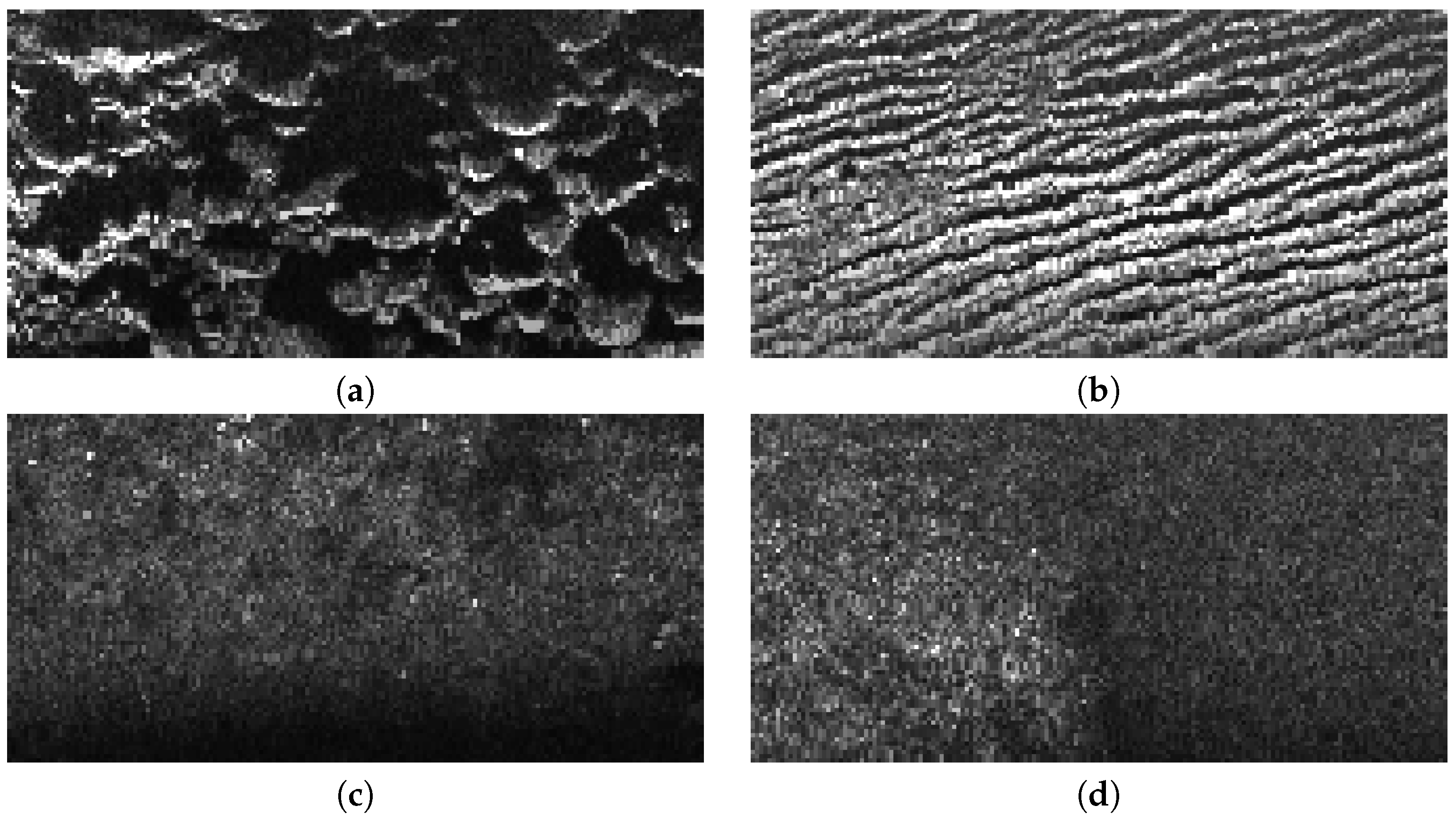
), and almost completely detected, with recalls larger than 92% in all cases and close to 95% in most of the cases. This is a reasonable result, since the class sand corresponds to rippled sand, which has the characteristic pattern shown in
Figure 10b, whilst the other classes encompass different textures. Nevertheless, both the class rock and the class others also lead to large precisions, recalls and F1-Scores.
When it comes to fall-out, sand is the class responsible for the worst results. Rock and others have fall-outs below 5% in all cases but sand depicts fall-outs ranging from 13% to 18%. This is likely to be due to the particular shapes in which the sand regions appear in the sea bottom. Whereas rocks and others appear in large regions, usually filling several consecutive swaths both on port and starboard, sand tends to be present in small banks. This means that the perimeter of the sand regions is large within the dataset in comparison to the perimeter of the other classes. Since the perimeter is the most difficult region to segment, even for a human when building the ground truth, the effects of these errors is more noticeable for the sand class.
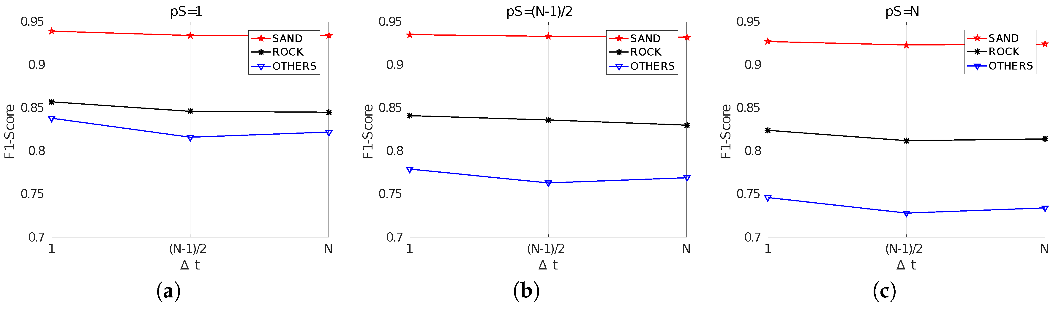
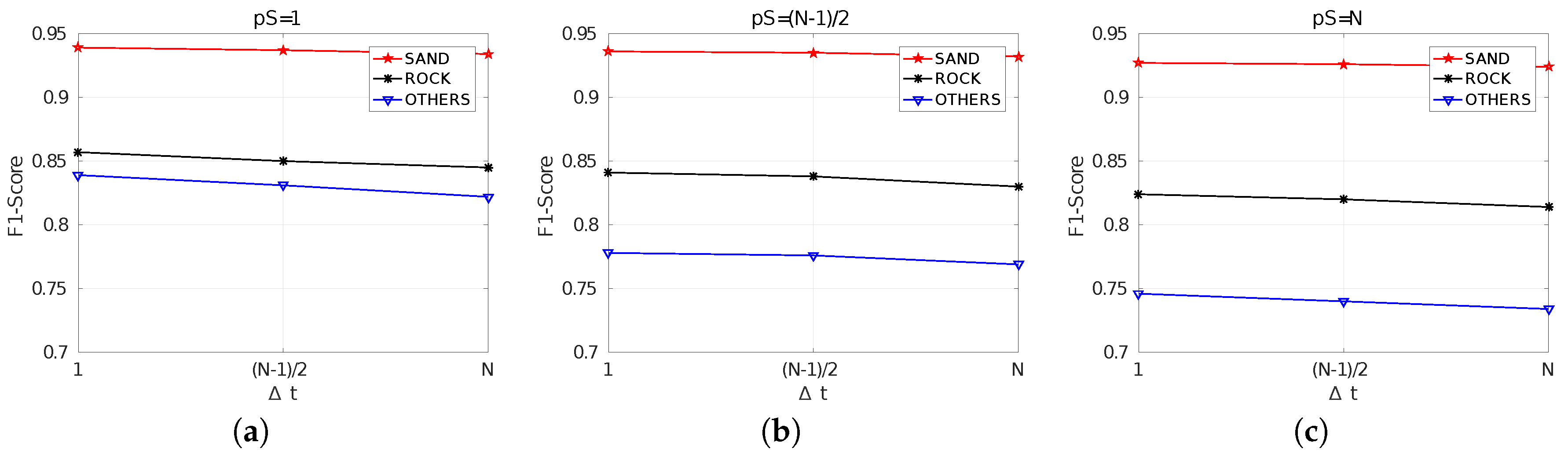
Figure 12 summarizes the obtained F1-Scores and facilitates the analysis of the effects of
. In particular, it can be observed how, independently of
, the differences in quality between
and
are really small and, in some cases, using
seems to lead to a small improvement. This suggests that values of
within the interval
barely influence the segmentation quality.
By comparing
Figure 12a–c it can be observed that the results are clearly affected by
, getting worse as
increases. It can also be observed how the quality differences between classes increases with
. Whereas the F1-Score of the sand class remains almost unchanged with
, the F1-Score of the class others is significantly affected. This suggests that using
seems to be the best choice.
The results corresponding to MCM are shown in
Table 7. These results are numerically similar to those obtained with SCM, and similar trends and patterns can be observed. Thus, the same analysis performed for SCM can be applied here.
However, interesting conclusions arise when observing the cases in which MCM surpasses SCM. These situations are those shown in gray cells in
Table 7, which mark the cases in which precision, recall, fallout and F1-Score values are larger for MCM and fall-out is smaller. The first aspect to emphasize is that differences, in all cases, are small. So, even though MCM improves SCM in some cases and leads to worse results in some others, the overall quality is almost the same.
The second aspect to emphasize, and probably the most relevant, is related to how the cases in which MCM improves SCM are distributed. For the sake of simplicity, let us focus on the F1-Score, though similar patterns appear with the other indicators.
As it can be observed, the improvements mostly depend on and are almost uncorrelated wit , which is reasonable since the use SCM or MCM has no effect during training. It can also be observed that for , MCM never surpasses SCM. However, this does not mean that MCM is worse in this case since the scores are exactly the same, within the working precision, for SCM and MCM. This is also reasonable, because means that the segmented patches do not overlap. Since the differences between SCM and MCM are the way in which overlapping regions are fused, no differences should appear in this case. It is important to emphasize that results are exactly the same in that case because the same trained model was used both for SCM and MCM since the data fusion method does not affect training.
Thus, the two interesting cases are and . For , even though MCM surpasses SCM only in two of nine cases, it actually leads to the same or almost the same results in the remaining seven cases. This means that when segmentation is performed for every new ping when the corresponding swath vector is available, the way in which overlapping regions are fused is not particularly relevant, probably because there is so much information that the fusion method does not make the difference.
However, when it comes fo , MCM surpasses SCM in all cases. The differences in this case are very small, but it is very significant that MCM is better independently on the training step and the class. Actually, the differences between this configuration and are larger for MCM than for SCM, showing how MCM is able to take profit of partially overlapping patches.
The F1-Scores are summarized in
Figure 13. Similarly to the SCM case (
Figure 12), results get worse and the differences between classes increase with the value of
, thus encouraging the use of
. In this case, however, the effects of
are perfectly clear, since in all cases the F1-Score gets worse with
. This is due to the already mentioned improvement when
using MCM with respect to the SCM case.
Previous discussion about the effects of and included the intuitive idea that small or would increase computational requirements. In order to quantify this intuition, both the training and the segmentation times have been measured on the provided Python implementation, which relies on Keras using TensorFlow as backend, executed on a standard laptop endowed with an i7 CPU at 3.1 GHz and without using neither GPU nor TPU.
Table 8 shows the results, which are graphically summarized in
Figure 14. The times, expressed in milliseconds, are the mean time per swath. More specifically, for each fold in the K-Fold cross-validation the training time has been measured and divided by the number of swaths or emitted pings in the training data corresponding to that fold. This training time has been averaged for all folds and the result is the training time per swath shown in the table.
As for the segmentation time, a similar procedure has been used. In this case the measured time is not only the NN prediction time but also the times spent to build the patch to segment, to put the segmented patch into the segmented image and to compute the most probable class when necessary have also been measured.
Since training is not affected neither by the value of
nor by the use of SCM or MCM, the NN was trained only once per value of
. That is why the training times are the same independently of
and the use of SCM or MCM, and that is the reason why a single plot of the training time as a function of
is provided in
Figure 14a. Results show how training time is particularly large when using
and is drastically reduced by increasing the patch separation. However, since training has to be performed only once, it should not be an relevant criterion to select one configuration or another.
Figure 14b,c clearly show that the segmentation time is not influenced by
. This is reasonable, since
only takes part in the training process. These figures also show a huge reduction in the segmentation time when switching from
to
but an almost negligible reduction when going from
to
. This is particularly interesting, since it means that choosing one of these two values of
can be done without taking the time into consideration.
By comparing SCM (
Figure 14b) and MCM (
Figure 14c) it is easy to see that, even though the segmentation times follow the same pattern, MCM is significantly more computationally demanding. For example, the smallest segmentation time when using SCM is 0.2148 ms whilst the smallest segmentation time with MCM is 0.6163 ms, which is almost three times larger.
Finally, it is important to emphasize that the segmentation times are really small in all cases. The worst situation, which happens when using MCM,
and
, requires 3.8411 ms per swath in average and the best one, which appears with SCM,
and
, uses 0.2145 ms per swath in average. This means that the system is able to process, depending on the configuration, between 260.342 and 4662.005 swaths per second in average. These frequencies are larger by far, in any case, to typical SSS sampling frequencies. For example, the used SSS provides 10 swaths per second, as shown in
Table 1.


