Zooplankton Distribution and Community Structure in the Pacific and Atlantic Sectors of the Southern Ocean during Austral Summer 2017–18: A Pilot Study Conducted from Ukrainian Long-Liners

Abstract

Preliminary results of the pilot study of the zooplankton in the region between the Ross and Scotia Seas from November 2017 to April 2018 are presented. In total, 53 zooplankton samples were collected in the top 100 m water layer using vertical tows of a 0.1 m² Juday net from four Ukrainian longliners operating during the Antarctic toothfish fishery. Total zooplankton abundance ranged from 3 to 2836 ind m⁻³ with a global mean of 360 ± 550 (±1 SD) ind m⁻³. The highest abundances were recorded at the northeastern Ross Sea. At those stations, small copepods (mainly Oithona spp., Oncaea spp., Ctenocalanus spp. and copepod nauplii) numerically dominated the samples. Total biomass ranged from 0.3 to 85 mg DW m⁻³ with a mean of 10.9 ± 14.5 mg DW m⁻³. The highest biomasses were recorded at the eastern Ross Sea, where pelagic tunicates Salpa thompsoni, siphonophores and ctenophora Callianira sp. accounted for >90% of total zooplankton biomass. At other stations, zooplankton biomass generally ranged from 5 to 20 mg DW m⁻³ with no clear pattern in distribution. The community composition was driven by the sampling latitude and/or season rather than longitudinally. This pilot study emphasized the unique opportunity to investigate zooplankton dynamics in the regions traditionally not sampled during the oceanographic surveys. It also created unprecedented opportunities to increase the seasonal and geographical zooplankton sampling coverage using ships of opportunity at a fraction of a dedicated oceanographic survey costs. The potential of such surveys are enormous in both providing invaluable information, contributing to existing long-term databases and enhancing an international collaboration in the Southern Ocean, particularly in light of recent modeling initiatives of the whole Antarctic system undertaken by the Commission for the Conservation of Antarctic Marine Living Resources.

1. Introduction

Zooplankton play a pivotal role in the world’s oceans, acting as a fundamental link between primary producers and top predators as well as commercially valuable fisheries [1,2,3]. Moreover, zooplankton contributes significantly to the biochemical cycling and export production affecting the cycling of carbon and other micro- and macronutrients in the ocean. It is a ubiquitous component of the biological pump mediating the organic matter removal from the surface to the deep ocean [4]. Zooplankton is a diverse group of organisms with crustacean plankton consistently dominating this group abundance and biomass [5]. Although zooplankton is extensively studied across marine environments, it is still poorly resolved in the biochemical and fisheries models. It is thus critical to gain a thorough understanding of the lower trophic level dynamics in pelagic ecosystems to be able to predict ecosystem responses under various climate change scenarios [6,7].

Since 1954, when A. de C. Baker [8] postulated the circum-Antarctic distribution of the Antarctic plankton, zooplankton has been repeatedly studied in the Atlantic (Antarctic Peninsula and Scotia Sea), Indian (Prydz Bay Region) and to a lesser extent in the Pacific (mainly the Ross Sea) sectors [5,9,10]. At the moment, we have a good understanding of species distribution patterns, biogeography, life cycles of major species, and long-term variability of the Antarctic pelagic ecosystems (see overview in [5,11]). Nevertheless, some regions of the Southern Ocean even today remain poorly sampled [12,13]. Historically, the area between the eastern parts of the Ross Sea and the Bellingshausen Sea in the Pacific Sector of the Southern Ocean receive little attention largely due to complicated logistics [12].

Recently, citizen science collections and observations, as well as ad-hoc sampling during commercial operations, have become a viable source of additional and often unique biological information at relatively low costs. While often such observations include only basic sampling, these collections provide important distributional data in areas that traditionally have been inadequately sampled, and improves seasonal and inter-annual coverage. During the 2017–18 season, the basic oceanographic data collections (as a pilot study) were carried out from long-line Ukrainian fishing boats during the licensed Antarctic toothfish fishery. This paper reports preliminary findings based on samples collected during austral summer in the poorly sampled coastal regions between the Ross and Bellingshausen seas as well as in the region east of the South Orkney Islands. The aims of this study were threefold: (a) to describe spatial and temporal zooplankton distribution; (b) to describe zooplankton composition; and (c) to investigate the development of the pelagic community in the top 100 m water layer.

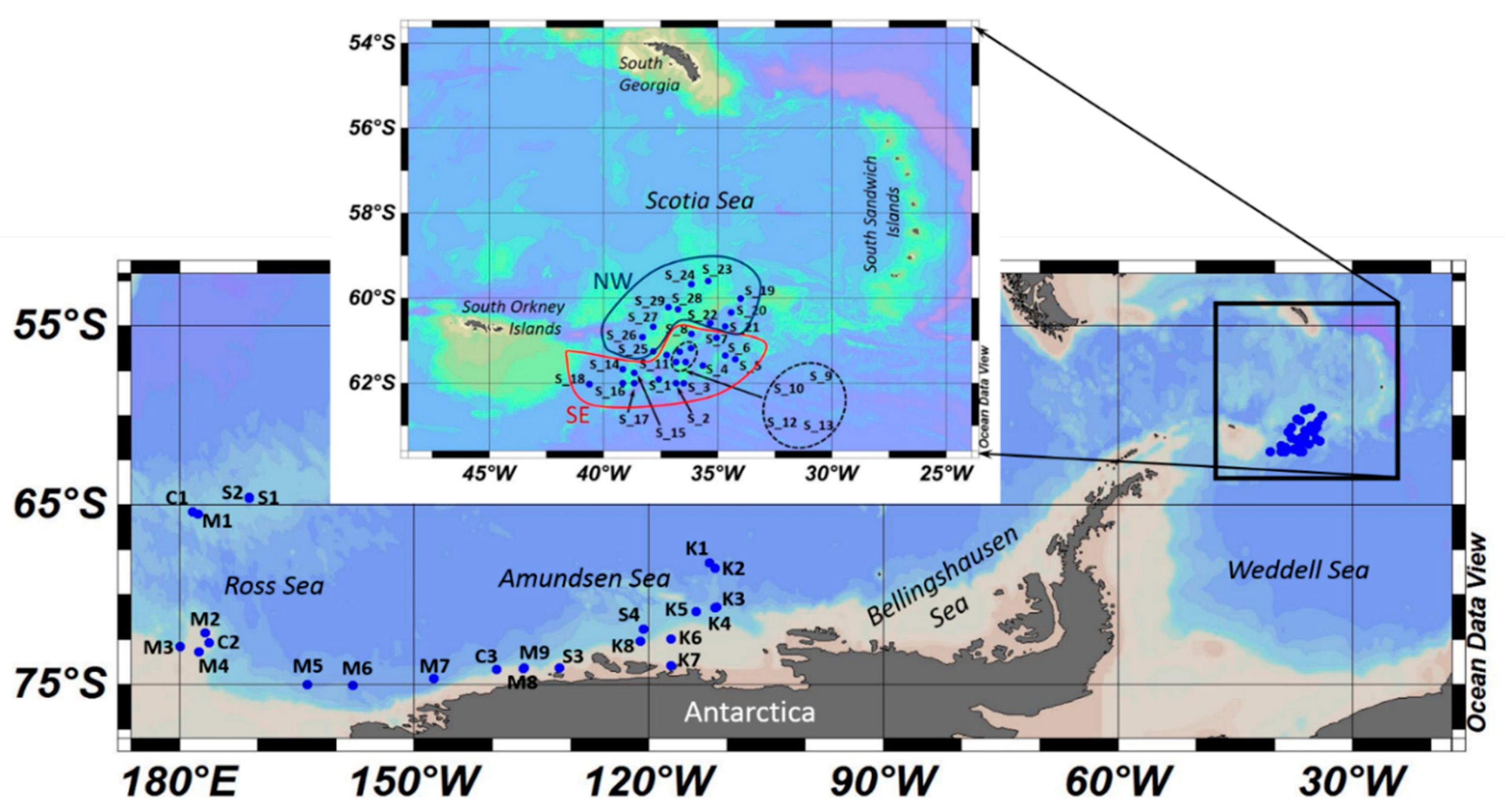
2. Materials and Methods

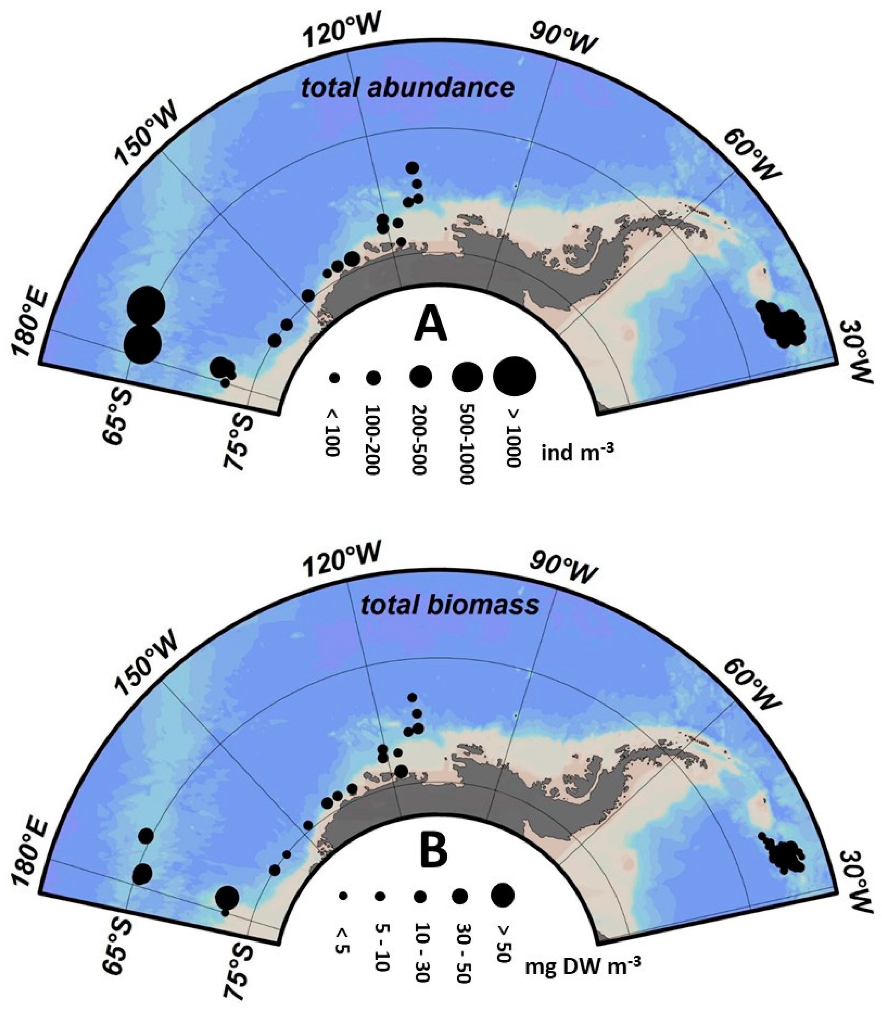
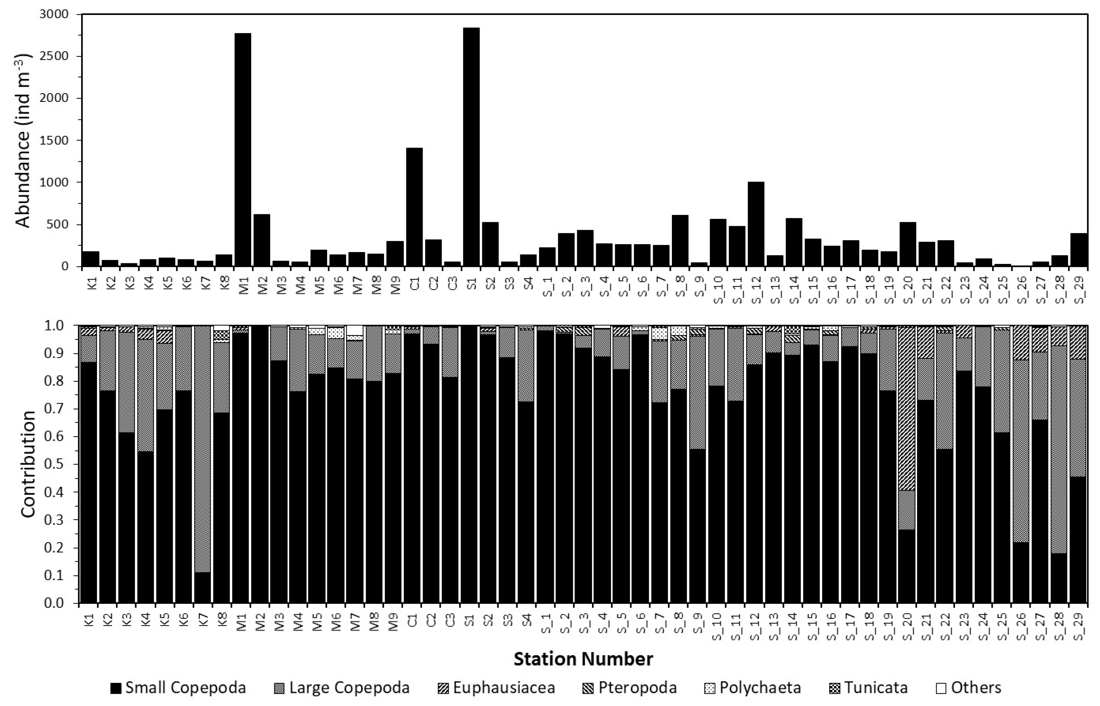
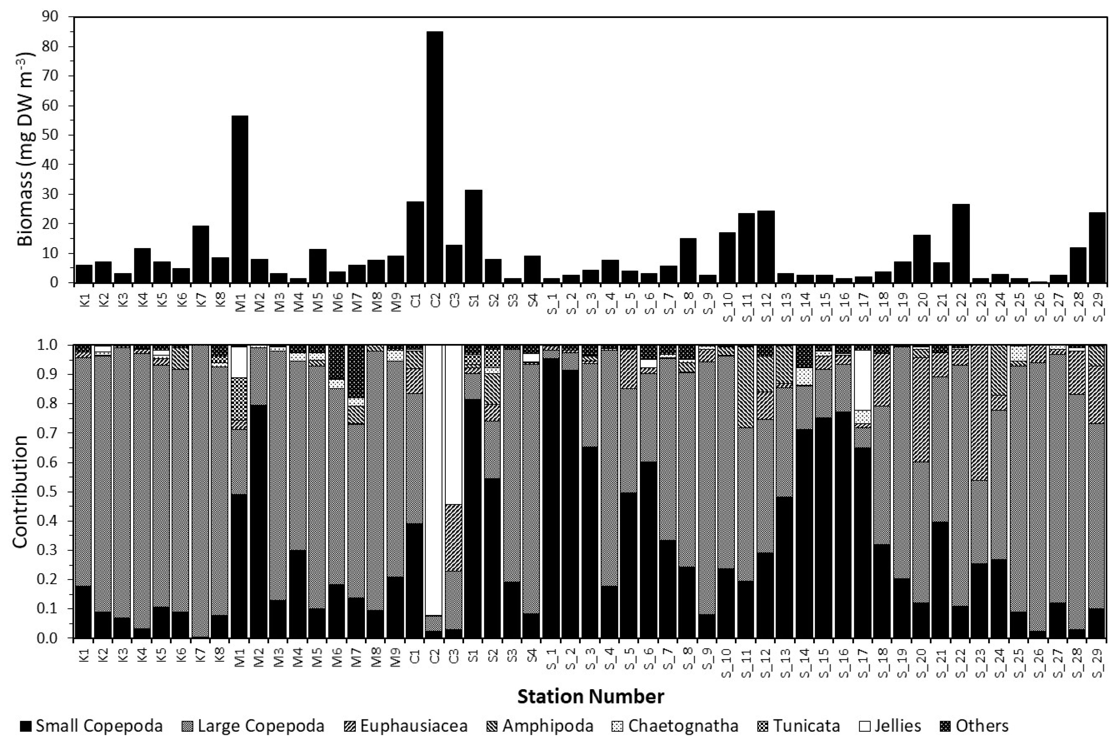
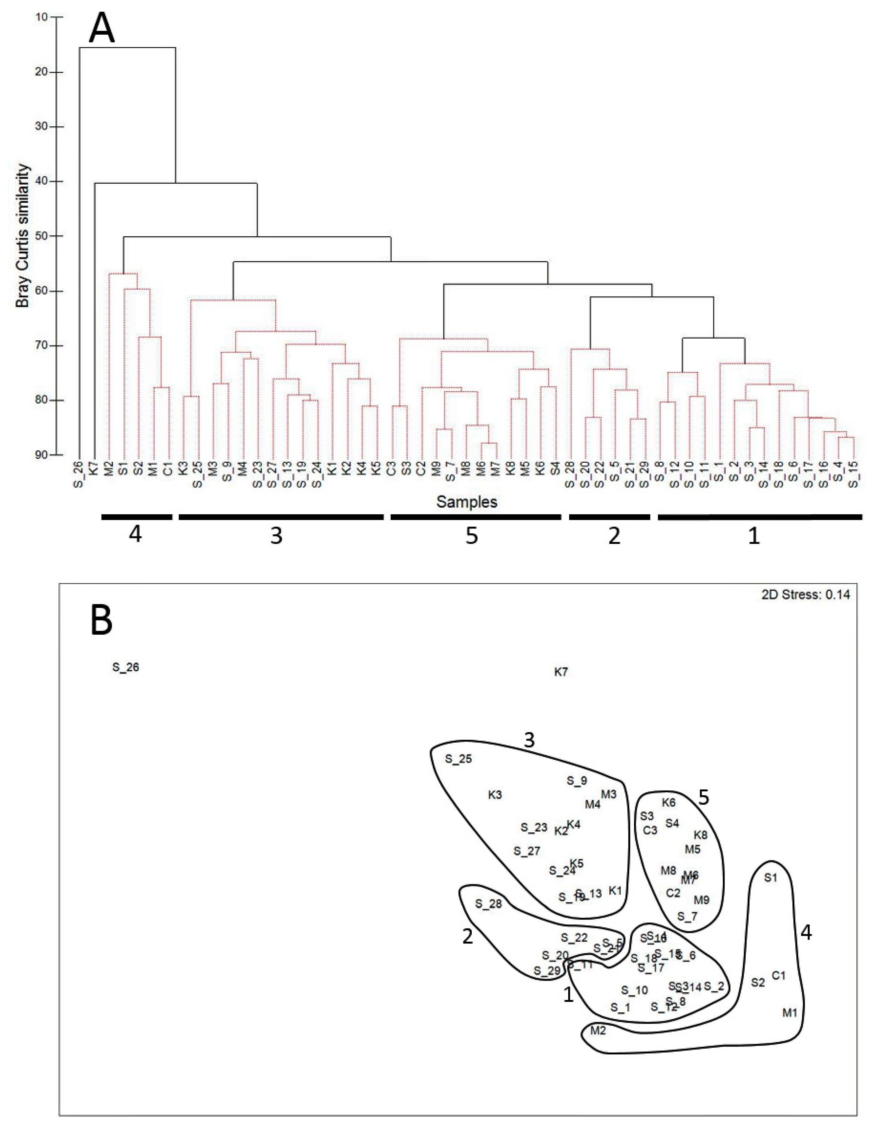
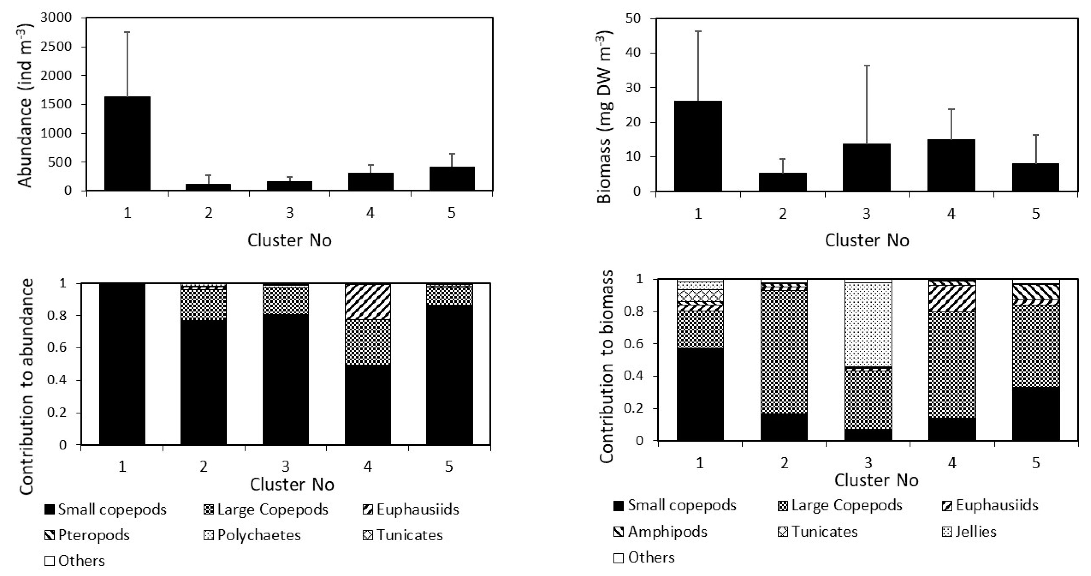
Data on zooplankton composition, distribution and density were collected in the Pacific and Atlantic sectors of the Southern Ocean during five voyages onboard four Ukrainian longliners: SRTM (medium fishing trawler, freezer stern trawler) Calypso, Koreiz, Marigolds, and Simeiz, between November 17, 2017 and April 10, 2018 (

Table 1. List of stations conducted onboard Ukrainian long-liners during austral summer 2017–2018 in the Pacific and Atlantic sectors of the Southern Ocean. Abbreviations: K, Koreiz; M, Marigolds; C, Calypso; S, Simeiz; nr, not recorded.

Station No.	Date	Time	Latitude (South)	Longitude (West)	Depth Sampled (m)	Volume Filtered, m3	SurfaceT °C
K1	11/17/2017	17:00	68.187	112.308	103	11.0	0.0
K2	11/21/2017	17:40	69.520	111.607	100	13.0	−1.0
K3	11/26/2017	17:00	70.672	111.422	104	10.5	−1.7
K4	12/3/2017	13:50	70.717	111.620	111	13.5	−1.8
K5	12/9/2017	17:20	70.917	113.965	125	13.0	−1.7
K6	12/14/2017	17:20	72.430	117.173	118	12.0	−1.8
K7	12/16/2017	12:35	73.932	117.172	141	20.0	−1.6
K8	1/28/2018	18:30	71.910	120.702	109	12.0	−1.6
M1	11/28/2017	11:25	65.503	177.599	101	10.5	nr
M2	1/16/2018	10:00	72.088	176.695	100	11.0	nr
M3	1/16/2018	17:00	72.872	179.983	100	11.0	nr
M4	1/17/2018	0:30	73.177	177.594	100	11.6	nr
M5	1/18/2018	9:10	75.008	163.665	100	10.0	nr
M6	1/18/2018	18:20	75.034	157.864	100	10.5	nr
M7	1/19/2018	10:50	74.638	147.513	100	11.0	nr
M8	1/21/2018	20:10	74.068	135.990	100	10.5	nr
M9	1/24/2018	19:50	74.068	131.488	100	10.5	nr
C1	12/12/2017	22:45	65.380	178.397	100	11.6	nr
C2	1/14/2018	16:20	72.648	176.247	100	10.2	nr
C3	1/18/2018	9:40	74.142	139.456	100	11.6	nr
S1	11/29/2017	18:00	64.573	171.133	113	12.0	nr
S2	12/1/2017	15:00	64.593	171.072	113	13.0	nr
S3	1/11/2018	21:35	74.112	136.119	118	13.0	nr
S4	1/28/2018	1:40	72.583	121.128	99	14.0	nr
S_1	2/27/2018	10:00	61.905	37.583	118	12.0	0.2
S_2	2/27/2018	14:30	62.000	36.833	122	13.0	0.0
S_3	2/27/2018	15:30	61.999	36.502	121	14.0	0.0
S_4	2/27/2018	19:30	61.583	35.667	122	13.0	0.0
S_5	2/27/2018	21:30	61.430	34.247	114	14.0	0.0
S_6	2/27/2018	23:00	61.350	34.673	112	13.0	0.0
S_7	2/28/2018	9:15	60.932	35.067	121	14.0	0.7
S_8	2/28/2018	11:15	60.833	36.167	118	12.0	1.5
S_9	2/28/2018	13:45	61.169	36.180	113	12.0	1.4
S_10	2/28/2018	15:30	61.257	36.669	113	12.0	1.6
S_11	2/28/2018	18:00	61.333	37.250	113	12.5	1.6
S_12	2/28/2018	20:30	61.500	36.833	104	12.0	1.5
S_13	2/28/2018	21:30	61.500	36.417	98	12.0	1.5
S_14	3/2/2018	12:40	61.667	39.167	109	11.0	1.4
S_15	3/2/2018	14:00	61.750	38.667	109	12.0	1.4
S_16	3/2/2018	16:20	61.998	39.168	106	11.0	1.4
S_17	3/2/2018	18:00	61.998	38.667	103	11.0	1.4
S_18	3/2/2018	21:10	62.017	40.634	103	11.0	1.4
S_19	3/31/2018	17:30	60.002	34.007	116	12.0	0.7
S_20	3/31/2018	19:30	60.333	34.417	108	11.0	0.7
S_21	3/31/2018	21:25	60.658	34.678	91	10.5	0.7
S_22	4/2/2018	21:10	60.583	35.333	100	11.0	0.8
S_23	4/8/2018	5:30	59.592	35.422	100	11.0	0.9
S_24	4/8/2018	9:20	59.672	36.167	104	12.0	1.0
S_25	4/10/2018	7:30	61.250	37.833	113	12.0	1.2
S_26	4/10/2018	13:20	60.916	38.298	108	11.0	1.2
S_27	4/10/2018	15:40	60.666	37.833	106	11.0	1.3
S_28	4/10/2018	20:20	60.255	36.752	100	11.0	1.4
S_29	4/10/2018	21:40	60.207	37.167	94	11.5	1.4

, Figure 1). Zooplankton vertical tows were performed mainly during the daylight using a Juday net with a mouth area of 0.1 m² and a mesh size of 100 µm. Nets were deployed generally to 100 m depth and retrieved at the speed of ≤1 ms⁻¹. The net filtering surface to mouth area ratio was ~5.5 and volume filtered was calculated multiplying the distance net travelled (wire length) by the mouth area. The volume filtered ranged from 10 to 20 m³ (Table 1). Zooplankton was preserved in a 4% buffered formaldehyde-seawater solution. At some stations, sea surface temperature was recorded (Table 1).

Zooplankton taxa were identified to the lowest taxonomic level when possible. For four major calanoid copepod species, Metrida gerlachei, Calanus propinquus, Calanoides acutus, and Rhincalanus gigas, all copepodite stages were identified. In the lab, the whole sample was initially processed by identifying, measuring, and counting all large (>10 mm) and rare (clearly visible <10 mm) organisms. The smallmouth area and fine mesh size likely significantly under-sampled large (>10 mm) organisms and their density estimates should be considered with caution. The remaining sample was processed either entirely if there where <200 individuals or sub-sampled (1/2 to 1/8) using a plankton splitter till approximately 200–300 individuals remained. This was used to quantify all organisms with the exception of small calanoids (Ctenocalanus and Clausocalanus), Oithona spp., Oncaea spp., Microsetella spp., copepod nauplii and crustacean eggs, which were counted in 5 mL sub-sample constituting 1/20 or 1/30 of the total sample. Abundance was calculated by dividing the count data by the proportion of the sample processed and then dividing the total count by the volume filtered and expressed as ind m⁻³. Biomass was calculated using conversions of zooplankton species and stage data to mg dry weight (DW) using [14] multiplied by the abundance data and expressed as mg DW m⁻³.

To compare plankton communities, a non-metric cluster and MDS analyses were performed using the Plymouth routines in multivariate ecological research (PRIMER 6; [15]) computer package according to the procedure described by Field et al. [16]. Species abundance data were log10(x + 1) transformed, and a station similarity matrix generated using the Bray–Curtis metric. Cluster analysis was then applied using group average sorting. To test for significant numerical differences between identified clusters and seasons, ANOVA was conducted on log-transformed abundance and biomass data [17].

MDS was performed on the similarity matrix. A SIMPROF test was conducted (α = 0.01) to determine statistical significance between clusters [15].

3. Results

3.1. Spatial Patterns in the Zooplankton Density and Composition

Total zooplankton abundance ranged from 2.9 to 2836 ind m⁻³ with a global mean of 360 ± 550 (±1SD) ind m⁻³. The highest abundances were recorded at the northeastern Ross Sea (Figure 2A). At those stations, small copepods (mainly Oithona spp., Oncaea spp., Ctenocalanus spp. and copepod nauplii) numerically dominated samples (Figure 3). At the remaining stations, zooplankton abundances usually varied between 100 and 500 ind m⁻³ with the tendency to increase from the west to the east (Figure 2A and Figure 3). With the exception of a few stations, small copepods accounted for >>60% of total abundance (Figure 3). The second most abundant group comprised of large calanoid copepods contributing from 10 to 40% of the total abundance. There was a tendency of increasing large copepod contributions at the northerly stations occupied in the Ross and the Scotia seas (Figure 3). It was also noted that the highest contributions and densities of small copepods coincided with the stations characterized by high phytoplankton concentrations. Phytoplankton concentration was not measured and inferred from phytoplankton dominating in zooplankton samples. The third-largest zooplankton group was composed of euphausiids accounting for 5 to 60% of total abundance. At the western stations, it was mostly presented by Thysanoessa macrura, while in the Scotia Sea, larval stages (mostly calyptopis 1) of Euphausia superba dominated reaching densities of 304 ind m⁻³ (Sta. S_20; Figure 3). Other groups combined seldom contributed more than 5% to the total zooplankton abundance.

Total biomass ranged from 0.3 to 85 mg DW m⁻³ with a mean of 10.9 ± 14.5 mg DW m⁻³. The highest biomasses were recorded at two stations (M1 and C2) of the eastern Ross Sea (Figure 2B). The first station was characterized by generally high concentrations of small and large copepods as well as pelagic tunicates, Salpa thompsoni, and siphonophores, while on the station C2, ctenophora Callianira sp. accounted for >90% of total zooplankton biomass (Figure 4). At other stations, zooplankton biomass generally ranged from 5 to 20 mg DW m⁻³ with no clear pattern in distribution (Figure 2B and Figure 4). Generally, at the stations with biomass levels <5 mg DW m⁻³, small copepods accounted for >60% of total biomass, while in the majority of stations, large calanoid copepods composed the largest proportion (range 3 to 99%) of total biomass (Figure 4). At some stations, other groups contributed significantly to total zooplankton biomass: e.g., euphausiids, up to 46% (Sta. S_23); amphipods, mainly Themisto gaudichaudii,—up to 28% (Sta. S_11); jellies—up to 54% (Sta. C3); chaetognaths, up to 6% (Sta. S_14) (Figure 4). A similar to abundance tendency of increasing euphausiid contributions from west to east was observed (Figure 4). Other groups combined generally contributed <<20% to the total zooplankton biomass.

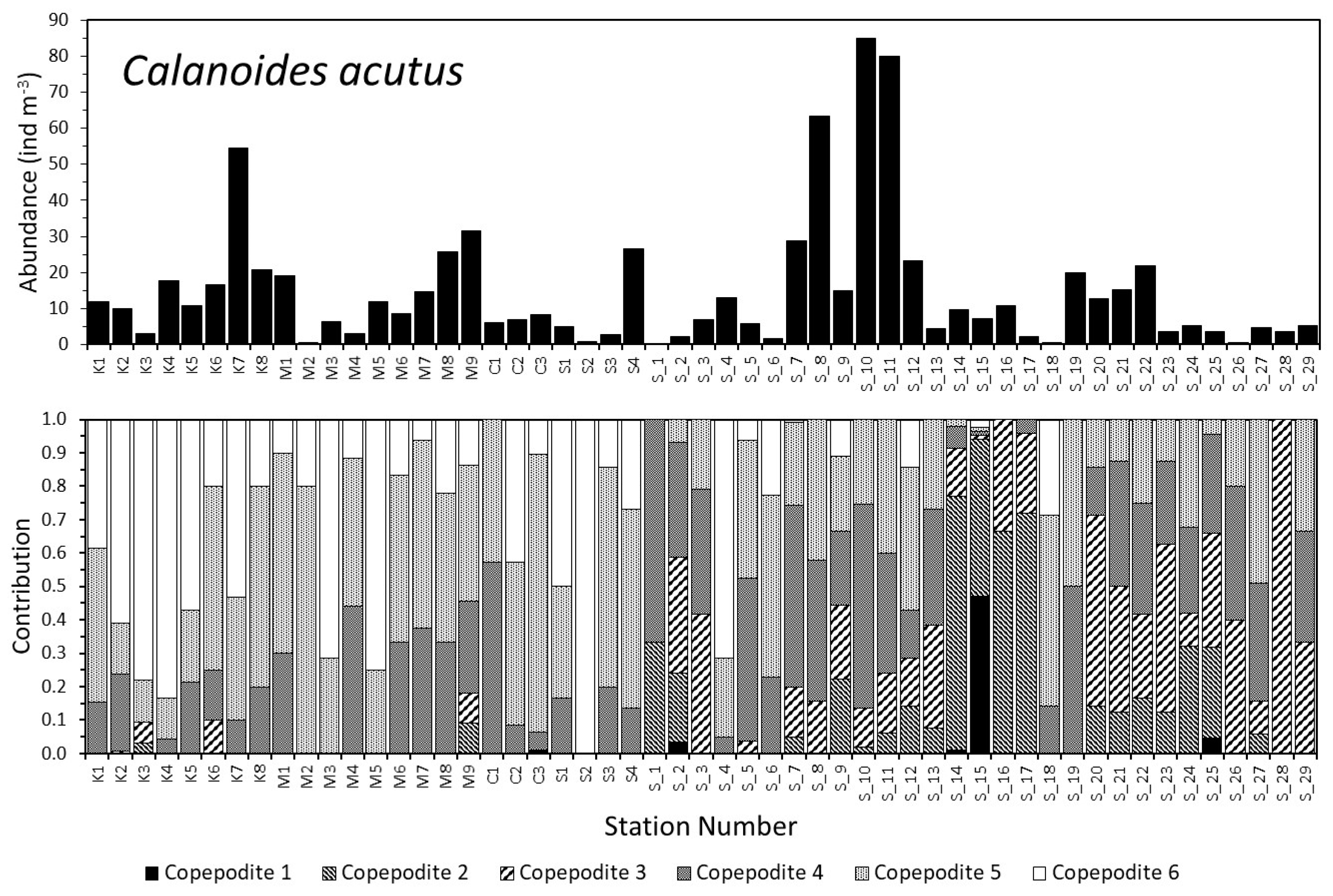
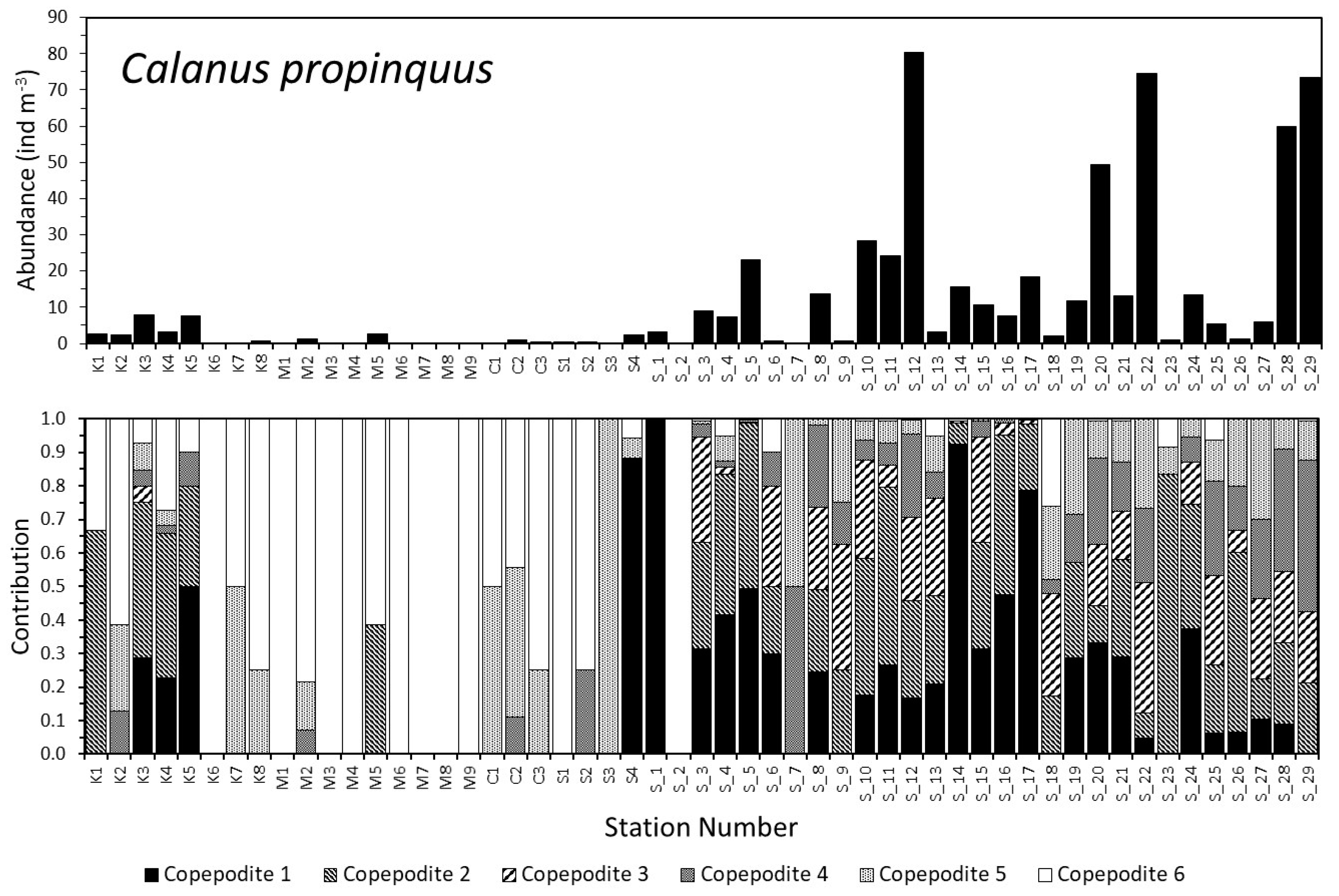
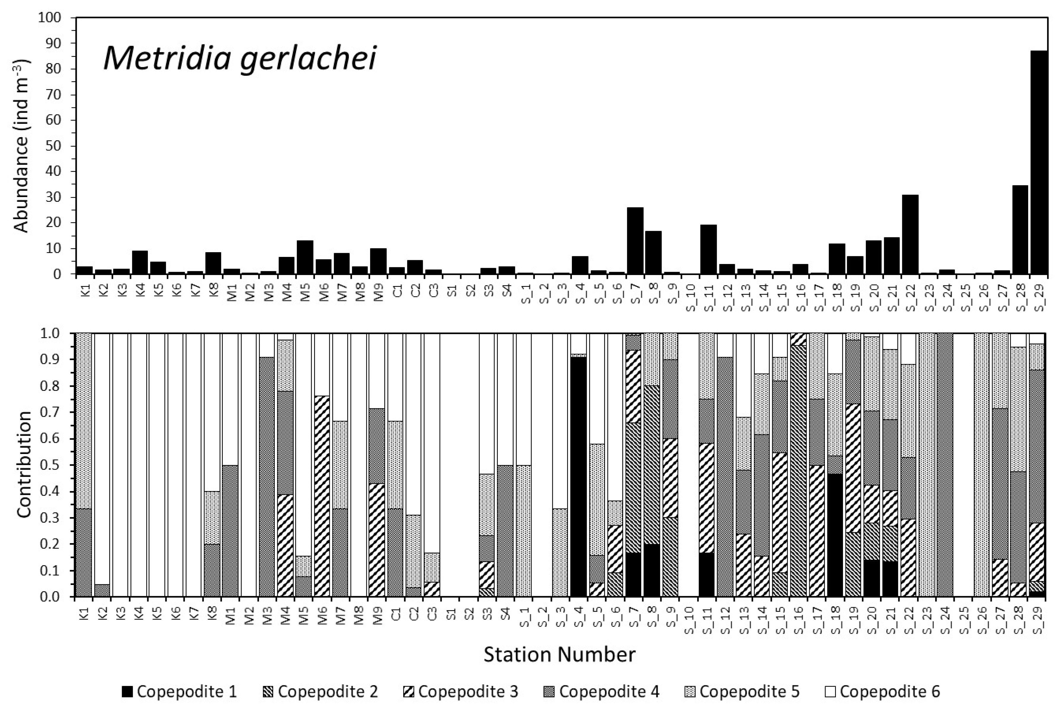
3.2. Dynamics of the Copepod Community

With several exceptions, total copepod density ranged between 100 and 300 ind m⁻³ and was generally higher in the Scotia Sea compared to the Ross Sea and Amundsen Sea stations (Figure 5). Nevertheless, three stations with the highest (>1000 ind m⁻³) copepod abundances were observed in the north-east Ross Sea. At all stations, small copepods dominated the samples: Oithona spp at Sta. S1, Oithona spp., Ctenocalanus spp., and copepod nauplii at Sta. M1; and with the addition of Oncaea spp. at Sta. C1 (Figure 5). Overall, Oithona spp. and copepod nauplii were prominent components of the copepod community (Figure 5). While Oncaea spp. contributed substantially in the southern stations of both Ross and Amundsen Seas, the north-western part of the Scotia Sea survey was nearly devoid of this species (Figure 5). Instead, the contribution of larger calanoids, e.g., C. propinquus, C. acutus, and M. gerlachei was significant.

Abundances of C. acutus, C. propinquus and M. gerlachei ranged from 0.3 to <90 ind m⁻³ (Figure 6, Figure 7 and Figure 8) with not significantly different means: 14.7 ± 18.3, 7.2 ± 13.6, and 11.2 ± 19.8 ind m⁻³, respectively. Both C. propinquus and M. gerlachei were mostly caught in the Scotia Sea (Figure 7 and Figure 8), while C. acutus was found across all regions (Figure 6). It was similar for all species as they all followed a seasonal progression in the development composition. Generally, copepodites 4–5 and adult individuals dominated at the Scotia and Ross Sea stations, with the exception of the north-east Ross Sea region (Figure 6, Figure 7 and Figure 8). Developing populations of all copepods (copepodites 1 to 4 dominated) were observed in the Scotia Sea during the survey conducted in February to March 2018 (Figure 6, Figure 7 and Figure 8).

Although seasonal patterns could only be studied across regions, it was possible to suggest that the highest, albeit highly variable, zooplankton abundance and biomass were observed in November (Figure 9). The overall pattern of seasonal densities showed a progressive decline from November to March despite the fact that differences between mean values were not significant (ANOVA, p > 0.05) (Figure 9).

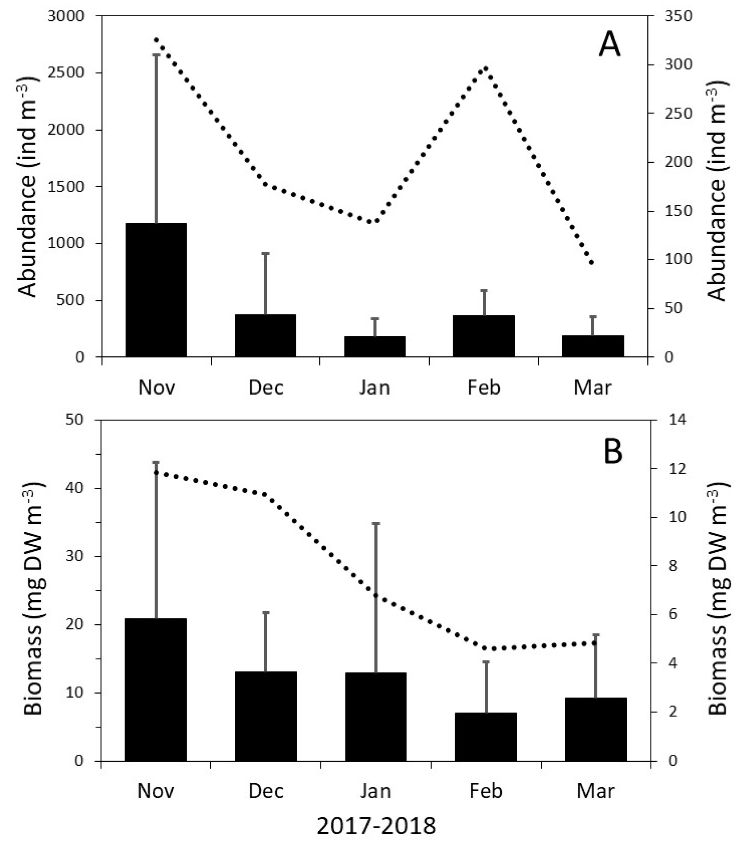
3.3. Community Composition Dynamics

Cluster analysis revealed five major station groupings and two outliers (Figure 10). Clusters 1 and 2, which were separated from each other at ~67% similarity, broadly corresponded to north western and south eastern Scotia Sea stations (Figure 1 and Figure 10A). Cluster 4 was separated at ~50% similarity and was composed of stations conducted in the northeast of the Ross Sea, while clusters 3 and 5, separated at ~55% similarity, included a mixture of the stations of all Ross, Amundsen and Scotia seas (Figure 1 and Figure 10A). These clusters were also visible using the MDS analysis (Figure 10B). The outliers were characterized by either very low zooplankton density or low diversity.

The total zooplankton abundance of cluster 1 was the highest and was significantly higher (ANOVA, p < 0.05) than total abundance in clusters 2 to 4, while clusters 2 to 5 abundances did not differ significantly (ANOVA, p > 0.05) (Figure 11;

Table 2. Species composition and densities of zooplankton communities identified using the cluster analysis presented in Figure 10A. Total abundance (A) and biomass (B) are expressed as ind m⁻³ and mg DW m⁻³, while numbers in columns are proportions.

Species	Cluster 1		Cluster 2		Cluster 3		Cluster 4		Cluster 5
	A	B	A	B	A	B	A	B	A	B
Calanoides acutus	0.4	5.3	9.9	50.4	10.3	27.6	3.4	6.8	5.2	36.6
Metridia gerlachei	0.1	0.4	3.3	6.3	4.4	5.1	9.5	6.1	1.1	1.4
Pleuromamma spp.	0	0	0.4	<0.1	0	0	<0.1	<0.1	0.1	<0.1
Ctenocalanus/Clausocalanus	13.6	20.2	10	5.5	6.2	1.8	15.9	8.1	8.2	10.3
Paraeuchaeta spp.	0	0	0.7	0.5	0.9	0.5	0.1	1.7	0.1	0.1
Euchirella rostromagna	0	0	0	0	0	0	<0.1	0.1	<0.1	0.1
Calanus propinquus	0	1.5	4.6	18.8	0.4	2.5	15.4	51.3	3.8	12.4
Calanus simillimus	0	1.8	0	0	0	0	0	0	0	0
Rhincalanus gigas	0.4	14.2	0.1	0.9	<0.1	0.2	<0.1	0.1	0.1	0.7
Oithona spp.	62.4	34.9	50.9	10.6	30.2	3.2	28.9	5.5	43.9	20.8
Oncaea spp.	3.5	1.1	2.3	0.3	35.1	2.1	1.1	0.1	5.5	1.4
Microsetella spp.	1.4	0.5	0.1	<0.1	0	0	0	0	0	0
Thysanoessa macrura	0.6	4.1	0.9	1.9	<0.1	0.1	0.5	5.7	0.1	2.2
Euphausia crystallorophias	0	0	0	0	<0.1	1.8	0	0	0	0
Euphausia superba	0	0	0.5	0.1	0	0	21	10.8	<0.1	0.8
Crustacea eggs	<0.1	<0.1	1.9	<0.1	<0.1	<0.1	1	<0.1	7.1	<0.1
Copepoda egg clusters	0	0	0	0	<0.1	<0.1	0	0	<0.1	<0.1
Copepoda nauplii	17.3	0.2	11.9	0.1	9.5	0	2.5	<0.1	22	0.2
Themisto gaudichaudii	0	0	<0.1	1.8	0	0	<0.1	2.3	<0.1	9.4
Vibilia antarctica	<0.1	2	0	0	0	0	0	0	0	0
Primno macropa	<0.1	<0.1	<0.1	<0.1	0	0	0	0	<0.1	0.1
Hyperiella dilatata	0	0.1	0	0	<0.1	0.4	0	0	0	0
Eusirus sp.	0	0	0	0	<0.1	0.2	0	0	0	0
Nematocarcinus spp.	0	0	<0.1	<0.1	0	0	0	0	0	0
Ostracoda	<0.1	0.2	<0.1	0.1	0.5	1	0.1	0.4	0.1	0.3
Spongiobranchaea australis	0	0	<0.1	<0.1	<0.1	<0.1	0	0	0	0
Clione antarctica	<0.1	0.6	<0.1	0.1	<0.1	<0.1	0	0	0.1	<0.1
Limacina helicina	<0.1	0.2	0.7	0.6	0.1	0.2	0.3	0.2	1.2	0.9
Rhinchonerella bongraini	<0.1	0.2	<0.1	0.1	0	0	0	0	0	0
Pelagobia longicerrata	0.1	0.1	1.3	0.6	1.4	0.5	0.1	0.2	0.9	1.2
Tomopteris spp.	<0.1	<0.1	<0.1	<0.1	0.1	<0.1	<0.1	<0.1	<0.1	<0.1
Sagitta gazellae	<0.1	<0.1	<0.1	0.1	<0.1	0.2	0	0	<0.1	<0.1
Eukrohnia hamata	<0.1	0.3	0.1	0.7	0.2	0.6	0.1	0.3	0.1	0.5
Medusae	<0.1	0.3	<0.1	0.4	0	0	0	0	<0.1	0.5
Appendicularia	0.1	0.1	0.1	<0.1	0.5	0.2	<0.1	<0.1	0.4	<0.1
Salpa thompsoni	0.1	7.2	0	0	0	0	0	0	0	0
Pyrostephos vanhoeffeni	<0.1	4.4	0	0	0	0	0	0	0	0
Calicopsis borchgervinki	0	0	0	0	<0.1	0.2	0	0	0	0
Calianira sp.	0	0	0	0	<0.1	51.7	<0.1	0.1	0	0
Total abundance (mean ± 1SD)	1620 ± 1124		121.0 ± 148.3		164.2 ± 86.6		317.5 ± 133.1		419.1 ± 218.8
Total biomass (mean ± 1SD)	26.2 ± 20.1		5.2 ± 4.1		13.8 ± 22.6		14.9 ± 9.0		8.0 ± 8.3

). Although a similar pattern was observed for total biomass, biomasses were not significantly different among clusters (Figure 11, Table 2).

SIMPROF routine confirmed that differences in composition between the five groupings, with the cluster and MDS analyses being significant (p < 0.01). Cluster 1 assemblage was numerically dominated (>95% of total abundance) by small copepods, mainly Oithona spp. (62%), copepod naluplii (17%), Ctenocalanus/Clausocalanus group (14%) and Oncaea spp. (4%) (Table 2); by biomass the same species dominated with the addition of R. gigas (14%), S. thompsoni (7%), T. macrura, and siphonophores (4% each) (Table 2, Figure 11). Clusters 2 and 3 had the lowest total abundance and by numbers dominated by small and large copepods (Figure 11). Cluster 2 assemblage was dominated (in descending order of species > 5% of abundance) by Oithona spp., copepod nauplii, Ctenocalanus/Clausocalanus, and C. acutus (Table 2). In terms of biomass, small copepods collectively accounted for ~ 16% of the standing stock, while large copepods dominated samples: C. acutus (50%), C. propinquus (19%), and M. gerlachei (6%) (Table 2). Cluster 3 assemblage, although numerically similar to previous one, had gelatinous, mostly cnidarian, zooplankton comprising most of the standing stock (52%), while large and small copepods accounted for ~30% and ~10%, respectively (Table 2, Figure 11). Assemblage belonging to cluster 4 was numerically dominated by small copepods followed by large copepods and euphausiids (Figure 11), but by biomass, large copepods, mainly C. propinquus (>50%), and calyptopis larvae of E. superba (11%) were most important contributors to the zooplankton standing stock (Figure 11; Table 2). Similar to cluster 1, numerically small copepods (>80%) followed by large copepods dominated cluster 5 assemblage (Figure 11). This cluster was different from others because amphipods, mainly Themisto gaudichaudii, contributed nearly 10% of the total zooplankton standing stock (Table 2).

4. Discussion

Presented data, in general, reflects the community composition and dynamic seasonal pattern of zooplankton in the region south of the Antarctic Convergence described in the literature [5,18,19,20,21]. It should however, be pointed out that while average densities and biomass levels were within the documented range, it was on the higher side of the estimates. This can be explained by a 100 µm mesh used in this study. In comparison, the majority of other estimates were obtained with nets equipped with mesh ≥200 µm [18,22,23,24,25]. It has been shown that in general, a 200 µm mesh net retains on average ~20% and ~40% less biomass and abundance, respectively, compared to a similarly designed 100 µm mesh net [26]. Indeed much higher (>5000 ind m⁻³) epipelagic zooplankton densities have also been documented, but those were coincident with high numbers of pteropods or euphausiid larvae [27,28,29]. Overall, the distribution of zooplankton varied considerably and generally had low abundances at the southernmost stations, while generally opposite trend was observed for total biomass. It is linked to the copepod community composition and occasional catch of a single macroplankton organism. In addition, closer to the continent, the majority large calanoid species dominated by adults ready for spawning.

There was no surprise that large copepods C. acutus, C. propinquus, and M. gerlachei generally dominated the zooplankton biomass and small copepods accounted for the majority of the zooplankton abundance in the top 100 m layer of water [5,19,30,31,32]. The macrozooplankton could have been largely under-sampled by the net with a small mouth area and fine mesh size that is designed to sample mesozooplankton. Following Baker’s [8] predictions, the community composition was differentiated according to the sampling latitude and/or season rather than longitudinally. The main composition of copepods and their development followed spatial and temporal patterns described by Voronina [33] for the whole Southern Ocean. Similar regional specifics have also been documented in various sectors of the Southern Ocean, e.g., the Ross Sea and western Amundsen Sea [10,13,27], the Weddell Sea [30,34,35], and the Cosmonaut Sea and the Prydz Bay Region [9,19,31,36,37,38].

A few observations are noteworthy. First, the substantial contribution of the pelagic tunicate S. thompsoni to the total abundance and biomass in the northeastern Ross Sea region. The salps were dominated by the small-sized blastozooids (aggregate forms), indicating recent asexual reproduction in the area, which was already ongoing in November 2017. This species was never encountered throughout the remaining survey until the end of the sampling season in April 2018. Second, while C. acutus was prominent across all surveys, both M. gerlachei and C. propinguus were most abundant and prevalent in the eastern part of the sampling area, particularly towards the austral fall. Third, there was a close coincidence, in both western and eastern surveys, of high small copepod numbers and samples dominated by the phytoplankton. While phytoplankton concentrations were not directly quantified, samples with large quantities of phytoplankton are a good proxy of the phytoplankton bloom conditions. Therefore, high quantities of small copepods and nauplii may have occurred either due to the net clogging at high phytoplankton concentrations that caused their better retention in the sample, or high phytoplankton densities could have been boosted copepod reproduction. We tend to favor the second explanation here. Fourth, Antarctic krill larvae were encountered only during the survey east of the South Orkney Islands. They had an unusually early developmental stage composition and were dominated by early (1 and 2) calyptopis stages, pointing to the late spawning season in 2017/18, which likely occurred at the beginning of March. The advanced stages (furcilia 1 to 3) were also present in the samples, but in very low numbers, and were likely indicators of spring/early summer krill spawning events. There is high uncertainty whether or not early krill larvae will be able to survive through the approaching winter, which may be a prerequisite for low krill recruitment during the next year. Finally, east of the South Orkney Islands, significant densities of the amphipod T. gaudichaudii were encountered; but was not observed in both the Ross and Amundsen Seas. Themisto is a carnivorous species contributing to mesozooplankton consumption [39,40]. It was also shown that this species might be an efficient predator on pelagic tunicates [41], thus responsible for decreasing zooplankton standing stock and salp population in the area.

In conclusion, it is important to emphasize that this pilot study opens new opportunities to investigate zooplankton dynamics using ships of opportunity in regions traditionally not sampled during the oceanographic surveys. These are preliminary results of the first such study, which could be further analyzed in-depth in follow up publications. Moreover, it will provide unprecedented opportunities to increase the seasonal and geographical zooplankton sampling coverage at a fraction of the cost of the full-scale oceanographic surveys. Such opportunities do not only provide invaluable information in regions that lack scientific efforts [12] but, more importantly, create an opportunity to establish and maintain international and hopefully long-term collaborations. In the end, such efforts would contribute a long way to supplement the already ongoing Southern Ocean continuous plankton recorder (SO-CPR) surveys and will be critical in monitoring long-term changes in the Southern Ocean pelagic ecosystem. Pilot studies like this could pave the way for building a long-term sampling program. Finally, a recently started initiative to model the Antarctic system will benefit from the additional information obtained in similar surveys.

References

1. Perry, R.I.; Batchelder, H.P.; Mackas, D.L.; Chiba, S.; Durbin, E.; Greve, W.; Verheye, H.M. Identifying global synchronies in marine zooplankton populations: Issues and opportunities. ICES J. Mar. Sci. 2004, 61, 445–456. [Google Scholar] [CrossRef] [Green Version]
2. Turner, J.T. The importance of small planktonic copepods and their roles in pelagic marine food webs. Zool. Stud. 2004, 43, 255–266. [Google Scholar]
3. Robert, D.; Murphy, H.M.; Jenkins, G.P.; Fortier, L. Poor taxonomical knowledge of larval fish prey preference is impeding our ability to assess the existence of a “critical period” driving year-class strength. ICES J. Mar. Sci. 2013, 71, 2042–2052. [Google Scholar] [CrossRef] [Green Version]
4. Steinberg, D.K.; Landry, M.R. Zooplankton and the Ocean Carbon Cycle. Annu. Rev. Mar. Sci. 2017, 9, 413–444. [Google Scholar] [CrossRef]
5. Atkinson, A.; Ward, P.; Hunt, B.P.V.; Pakhomov, E.A.; Hosie, G.W. An overview of Southern Ocean zooplankton data: Abundance, biomass, feeding and functional relationships. CCAMLR Sci. 2012, 19, 171–218. [Google Scholar]
6. Mantua, N.J.; Hare, S.R.; Zhang, Y.; Wallace, J.M.; Francis, R.C. A Pacific interdecadal climate oscillation with impacts on salmon production. Bull. Am. Meteorol. Soc. 1997, 78, 1069–1080. [Google Scholar] [CrossRef]
7. Rogers, A.; Frinault, B.; Barnes, D.; Bindoff, N.; Downie, R.; Ducklow, H.; Friedlaender, A.; Hart, T.; Hill, S.; Hofmann, E.; et al. Antarctic Futures: An Assessment of Climate-Driven Changes in Ecosystem Structure, Function, and Service Provisioning in the Southern Ocean. Annu. Rev. Mar. Sci. 2020, 12, 87–120. [Google Scholar] [CrossRef] [Green Version]
8. Baker, A.D.C. The circumpolar continuity of Antarctic plankton species. Discov. Rep. 1954, 27, 201–2018. [Google Scholar]
9. Makabe, R.; Tanimura, A.; Tamura, T.; Hirano, D.; Shimada, K.; Hashihama, F.; Fukuchi, M. Meso-zooplankton abundance and spatial distribution off Lützow-Holm Bay during austral summer 2007–2008. Polar Sci. 2017, 12, 25–33. [Google Scholar] [CrossRef]
10. Smith, W.O.; Delizo, L.M.; Herbolsheimer, C.; Spencer, E. Distribution and abundance of mesozooplankton in the Ross Sea, Antarctica. Polar Biol. 2017, 40, 2351–2361. [Google Scholar] [CrossRef]
11. Steinberg, D.K.; Ruck, K.E.; Gleiber, M.R.; Garzio, L.M.; Cope, J.S.; Bernard, K.S.; Stammerjohn, S.E.; Schofield, O.M.E.; Quetin, L.B.; Ross, R.M. Long-term (1993–2013) changes in macrozooplankton off the Western Antarctic Peninsula. Deep Sea Res. Part I Oceanogr. Res. Pap. 2015, 101, 54–70. [Google Scholar] [CrossRef]
12. Moriarty, R.; O’Brien, T.D. Distribution of mesozooplankton biomass in the global ocean. Earth Syst. Sci. Data 2013, 5, 45–55. [Google Scholar] [CrossRef] [Green Version]
13. Yang, E.J.; Lee, Y.; Lee, S. Trophic interactions of micro- and mesozooplankton in the Amundsen Sea polynya and adjacent sea ice zone during austral late summer. Prog. Oceanogr. 2019, 174, 117–130. [Google Scholar] [CrossRef]
14. Mizdalski, E. Weight and length data of zooplankton in the Weddell Sea in austral spring 1986 (ANT V/3). Ber. Polarforsch. 1988, 55, 1–72. [Google Scholar]
15. Clarke, K.R.; Warwick, R.M. Change in Marine Communities: An Approach to Statistical Analysis and Interpretation, 2nd ed.; PRIMAR-E: Plymouth, UK, 2001. [Google Scholar]
16. Field, J.; Clarke, K.R.; Warwick, R. A Practical Strategy for Analysing Multispecies Distribution Patterns. Mar. Ecol. Prog. Ser. 1982, 8, 37–52. [Google Scholar] [CrossRef]
17. Zar, J.H. Biostatistical Analysis, 4th ed.; Prentice Hall: Upper Saddle River, NJ, USA, 1999. [Google Scholar]
18. Stevens, C.J.; Pakhomov, E.A.; Robinson, K.V.; Hall, J.A. Mesozooplankton biomass, abundance and community composition in the Ross Sea and the Pacific sector of the Southern Ocean. Polar Biol. 2014, 38, 275–286. [Google Scholar] [CrossRef]
19. Swadling, K.M.; Kawaguchi, S.; Hosie, G.W. Antarctic mesozooplankton community structure during BROKE-West (30° E–80° E), January–February 2006. Deep Sea Res. Part II Top. Stud. Oceanogr. 2010, 57, 887–904. [Google Scholar] [CrossRef]
20. Takahashi, K.T.; Hosie, G.W.; Odate, T. Intra-annual seasonal variability of surface zooplankton distribution patterns along a 110° E transect of the Southern Ocean in the austral summer of 2011/12. Polar Sci. 2017, 12, 46–58. [Google Scholar] [CrossRef]
21. Takahashi, K.T.; Ojima, M.; Tanimura, A.; Odate, T.; Fukuchi, M. The vertical distribution and abundance of copepod nauplii and other micro- and mesozooplankton in the seasonal ice zone of Lützow-Holm Bay during austral summer 2009. Polar Biol. 2016, 40, 79–93. [Google Scholar] [CrossRef]
22. Voronina, N.M.; Kosobokova, K.N.; Pakhomov, E.A. Size structure of Antarctic metazoan plankton according to united net, trawl and water bottle data. Russ. J. Aquat. Ecol. 1994, 3, 137–142. [Google Scholar]
23. Voronina, N.M.; Kosobokova, K.N.; Pakhomov, E.A. Composition and biomass of summer metazoan plankton in the 0–200 m layer of the Atlantic sector of the Antarctic. Polar Biol. 1994, 14, 91–95. [Google Scholar] [CrossRef]
24. Errhif, A.; Razouls, C.; Mayzaud, P. Composition and community structure of pelagic copepods in the Indian sector of the Antarctic Ocean during the end of the austral summer. Polar Biol. 1997, 17, 418–430. [Google Scholar] [CrossRef]
25. Boysen-Ennen, E.; Hagen, W.; Hubold, G.; Piatkowski, U. Zooplankton biomass in the ice-covered Weddell Sea, Antarctica. Mar. Biol. 1991, 111, 227–235. [Google Scholar] [CrossRef]
26. Gallienne, C.P.; Robins, D.B. Is Oithona the most important copepod in the world’s oceans? J. Plankton Res. 2001, 23, 1421–1432. [Google Scholar] [CrossRef]
27. Makarov, R.R.; Men’shenina, L.L.; Spiridonov, V.A. Plankton distribution and its seasonal biological activity in the central and western parts of the Antarctic Pacific Sector. In Oceanographic and Biological Investigations of the Pacific Antarctic Sector (Biologo-Okeanographicheskie Issledovanija Tihookenaskogo Sektora Antaktiki); Makarov, R.R., Dolzhenkov, V.N., Ljubimova, T.G., Spiridonov, V.A., Tarverdieva, T.G., Eds.; VNIRO Publishers: Moscow, Russia, 1987; pp. 90–110. (In Russian) [Google Scholar]
28. Pane, L.; Feletti, M.; Francomacaro, B.; Mariottini, G.L. Summer coastal zooplankton biomass and copepod community structure near the Italian Terra Nova Base (Terra Nova Bay, Ross Sea, Antarctica). J. Plankton Res. 2004, 26, 1479–1488. [Google Scholar] [CrossRef] [Green Version]
29. Hunt, B.; Pakhomov, E.; Hosie, G.; Siegel, V.; Ward, P.; Bernard, K. Pteropods in Southern Ocean ecosystems. Prog. Oceanogr. 2008, 78, 193–221. [Google Scholar] [CrossRef]
30. Hopkins, T.L.; Torres, J.J. The zooplankton community in the vicinity of the ice edge, western Weddell Sea, March 1986. Polar Biol. 1988, 9, 79–87. [Google Scholar] [CrossRef]
31. Hosie, G.W.; Cochran, T.G.; Pauly, T.; Beaumont, K.L.; Wright, S.W.; Kitchener, J.A. The zooplankton community structure of Prydz bay, January–February 1993. Proc. NIPR Symp. Polar Biol. 1997, 10, 90–133. [Google Scholar]
32. Yang, G.; Li, C.; Sun, S. Inter-annual variation in summer zooplankton community structure in Prydz Bay, Antarctica, from 1999 to 2006. Polar Biol. 2011, 34, 921–932. [Google Scholar] [CrossRef]
33. Voronina, N.M. Pelagic Ecosystems of the Southern Ocean; Nauka Press: Moscow, Russia, 1984; p. 206. (In Russian) [Google Scholar]
34. Fedotova, V.V.; Gorlanova, O.L. Peculiarities of the mesoplankton distribution in the Ross Sea in summer 1983. In Oceanographic and Biological Investigations of the Antarctic Pacific Sector (Biologo-Okeanographicheskie Issledovanija Tihookenaskogo Sektora Antaktiki); Makarov, R.R., Dolzhenkov, V.N., Ljubimova, T.G., Spiridonov, V.A., Tarver-dieva, T.G., Eds.; VNIRO Publishers: Moscow, Russia, 1987; pp. 80–90. (In Russian) [Google Scholar]
35. Makarov, R.R.; Solyankin, E.V. Abundant copepods and regional peculiarities of their seasonal development in the east area of the Weddell Gyre. In Investigations of the Weddell Gyre. Oceanographic Conditions and Peculiarities of the Development of Plankton Communities; Solyankin, E.V., Ed.; VNIRO Press: Moscow, Russia, 1990; pp. 99–125. (In Russian) [Google Scholar]
36. Bundichenko, E.V.; Khromov, N.S. Mesoplankton biomass, age composition and distribution of dominant species in relation to water structure in the Commonwealth and the Cosmonaut Seas. In Interdisciplinary Investigations of Pelagic Ecosystem in the Commonwealth and Cosmonaut Seas; Lubimova, T.G., Makarov, R.R., Maslennikov, V.V., Samyshev, E.Z., Bibik, V.A., Tarverdieva, T.G., Eds.; VNIRO Publishers: Moscow, Russia, 1988; pp. 83–109. (In Russian) [Google Scholar]
37. Bunichenko, E.V. Change in age composition of the abundant copepod species in the Cooperation Sea in 1977–1990. Oceanol. Russ. Acad. Sci. 1994, 34, 252–258. (In Russian) [Google Scholar]
38. Yang, G.; Li, C.; Wang, Y.; Zhang, Y. Vertical profiles of zooplankton community structure in Prydz Bay, Antarctica, during the austral summer of 2012/2013. Polar Biol. 2017, 40, 1101–1114. [Google Scholar] [CrossRef]
39. Pakhomov, E.A.; Perissinotto, R. Trophodynamics of the hyperiid amphipod Themisto gaudichaudii in the South Georgia region during late austral summer. Mar. Ecol. Prog. Ser. 1996, 134, 91–100. [Google Scholar] [CrossRef] [Green Version]
40. Froneman, P.W.; Pakhomov, E.A.; Treasure, A. Trophic importance of the hyperiid amphipod, Themisto gaudichaudii, in the Prince Edward Archipelago (Southern Ocean) ecosystem. Polar Biol. 2000, 23, 429–436. [Google Scholar] [CrossRef]
41. Kruse, S.; Pakhomov, E.A.; Hunt, B.; Chikaraishi, Y.; Ogawa, N.; Bathmann, U. Uncovering the trophic relationship between Themisto gaudichaudii and Salpa thompsoni in the Antarctic Polar Frontal Zone. Mar. Ecol. Prog. Ser. 2015, 529, 63–74. [Google Scholar] [CrossRef]
Figure 1. Sample collections carried out from Ukrainian long-liners during austral summer 2017–2018 in the Pacific and Atlantic sectors of the Southern Ocean. In the insert, SIMEIZ collections, NW, northwestern South Orkney Islands (27 February to 3 March, 2018); SE, southeastern South Orkney Islands (31 March to 10 April, 2018). Station abbreviations: K, Koreiz collections (17 November, 2017 to 28 January, 2018); M, Marigolds collections (28 November, 2017 to 24 January, 2018); C, Calypso collections (12 December, 2017 to 18 January, 2018); S, Simeiz collections (29 November, 2017 to 28 January, 2018).
Jmse 08 00488 g001
Figure 2. Spatial distribution of total zooplankton abundance (A, ind m−3) and biomass (B, mg DW m−3) in the upper 100 m layer during austral summer 2017–2018 in the Pacific and Atlantic sectors of the Southern Ocean.
Jmse 08 00488 g002
Figure 3. Zooplankton total abundance (upper panel) and contribution of major taxonomic groups (lower panel) in the Pacific and Atlantic sector of the Southern Ocean during austral summer 2017–18.
Jmse 08 00488 g003
Figure 4. Zooplankton total biomass (upper panel) and contribution of major taxonomic groups (lower panel) in the Pacific and Atlantic sector of the Southern Ocean during austral summer 2017–18.
Jmse 08 00488 g004
Figure 5. Copepod community total abundance (upper panel) and species contributions (lower panel) in the Pacific and Atlantic sector of the Southern Ocean during austral summer 2017–18.
Jmse 08 00488 g005
Figure 6. Calanoides acutus abundance (upper panel) and developmental stage composition (lower panel) in the Pacific and Atlantic sector of the Southern Ocean during austral summer 2017–18.
Jmse 08 00488 g006
Figure 7. Calanus propinquus abundance (upper panel) and developmental stage composition (lower panel) in the Pacific and Atlantic sector of the Southern Ocean during austral summer 2017–18.
Jmse 08 00488 g007
Figure 8. Metridia gerlachei abundance (upper panel) and developmental stage composition (lower panel) in the Pacific and Atlantic sector of the Southern Ocean during austral summer 2017–18.
Jmse 08 00488 g008
Figure 9. Seasonal dynamics of zooplankton abundance (A) and biomass (B) in the upper 100 m layer during austral summer 2017–2018 in the Pacific and Atlantic sectors of the Southern Ocean. Bars with 1 SD illustrate the arithmetic mean densities (left axis), the dotted line shows the geometric mean (right axis).
Jmse 08 00488 g009
Figure 10. Cluster (A) and MDS (B) analyses of zooplankton collections (by species abundance only) in the southern parts of the Pacific and Atlantic sectors of the Southern Ocean during austral summer 2017–18.
Jmse 08 00488 g010
Figure 11. Zooplankton total abundance (left panels) and biomass (right panels), as well as taxonomic group composition (bottom panels, respectively), in the Pacific and Atlantic sector of the Southern Ocean during austral summer 2017–18 in clusters identified in Figure 10A.
Jmse 08 00488 g011