A Mesh Deformation Method for CFD-Based Hull form Optimization

Abstract

Computational fluid dynamics (CFD) is an effective tool for ship resistance prediction and hull form optimization. A three-dimensional volume mesh is essential for CFD simulation, and mesh generation requires much time and effort. Mesh deformation can reduce the time for mesh generation and simulation. The radial basis function (RBF) and inverse distance weighted (IDW) methods are well-known mesh deformation methods. In this study, the two methods are compared and a novel mesh deformation method for hull form optimization is proposed. For the comparison, a circular cylinder polyhedral mesh was deformed to the National Advisory Committee for Aeronautics (NACA) 0012 mesh. The results showed that the RBF method is faster than the IDW method, but the deformed mesh quality using the IDW method is better than that using the RBF method. Thus, the RBF method was modified to improve the deformed mesh quality. The centroids of the boundary layer cells were added to the control points, and the displacements of the centroids were calculated using the IDW method. The cells far from the ship were aligned to the free surface to minimize the numerical diffusion of the volume of fluid function. Therefore, the deformable region was limited by the deformed boundary, which reduced the time required for mesh deformation. To validate its applicability, the proposed method was applied for varying the bow shape of Japan Bulk Carrier (JBC). The resistances were calculated with the deformed meshes. The calculation time was reduced to approximately one-third using the result of the initial hull form as the initial condition. Thus, the proposed mesh deformation method is efficient and effective enough for CFD-based hull form optimization.

1. Introduction

Computational fluid dynamics (CFD) is one of the general tools for estimating the resistance of a ship in calm water. Naval architects iterate the hull form variation, grid generation, and CFD calculation to minimize the resistance. Even though the hull form variation is extremely localized and low, the grid must be regenerated. Many shipbuilding and design companies are exerting efforts to automate the procedure to reduce the time and cost. Moreover, many studies on CFD-based design optimization have been conducted. An optimization algorithm to minimize the iterations is the most important and the hull form variation method according to the design parameter is very essential.

Kim and Yang [1] applied two surface modification methods for hull form optimization. One was based on a radial basis function (RBF), while the other was based on a sectional area curve. Kim and Yang’s [1] RBF method uses only 6 control points as design variables to minimize the resistance of Korea Research Institute for Ships and Ocean Engineering (KRISO) Container Ship (KCS) in three speeds. The resistance of the modified hull was evaluated using a method based on the Neumann–Michell theory, which uses only a surface mesh. Kim et al. [2] applied the same method used by Kim and Yang [1] to improve the resistance and seakeeping performance of the US Navy surface combatant David Taylor Model Basin (DTMB) 5415. Mahmood and Huang [3] optimized a bulbous bow to minimize the total resistance using a genetic algorithm. They used ANSYS FLUENT and GAMBIT (Ansys, In., Canonsburg, PA, USA) for resistance calculation and mesh generation, respectively. A GAMBIT journal file was created to automate the hull form variation and volume mesh generation in accordance with the design parameters. Zhang et al. [4] proposed an improved particle swarm optimization algorithm, where Siemens STAR-CCM+ (Siemens Industry Software Ltd., Plano, TX, USA) was used for volume mesh generation and resistance calculation. The hull form was varied using an arbitrary shape deformation (ASD) technique proposed by Sun et al. [5]. The ASD technique is based on a B-spline and requires that the volume is set up outside the body with many control points and connections.

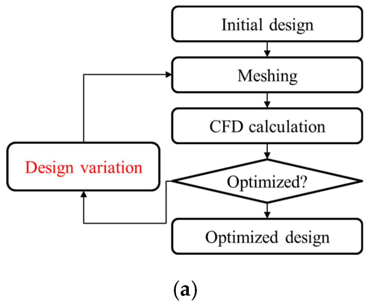
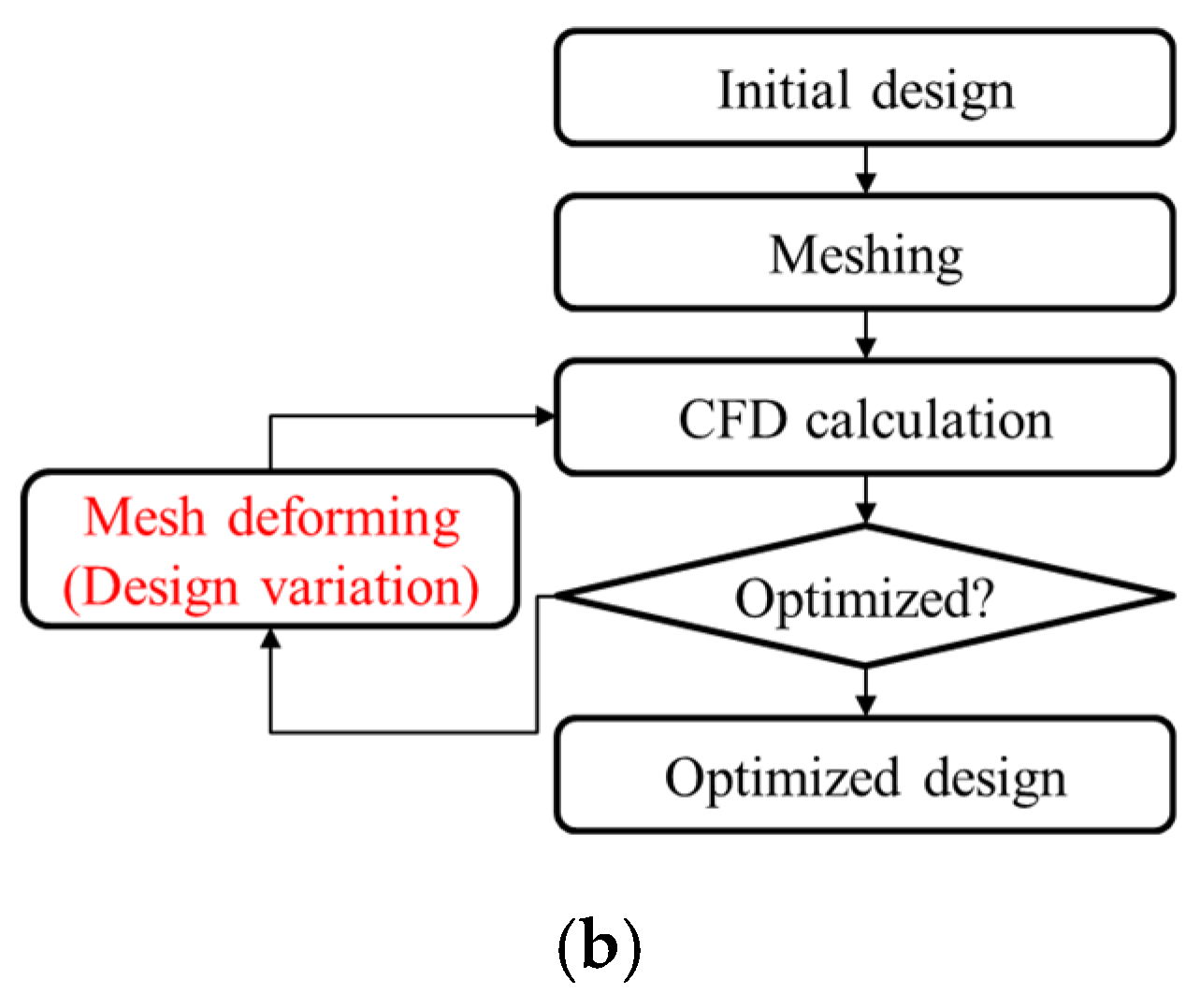
The volume mesh deforming method has been developed to simplify the optimization process and reduce the turnaround time as shown in Figure 1. Mesh deformation is much faster than grid generation, and the simulation with a deformed mesh uses the results of the original mesh as the initial condition. Successive calculation also reduces the calculation time. Morris et al. [6] developed a mesh deformation method based on the RBF method. The control points of the RBF method were used as design parameters. The method was independent of both the flow solver and grid generator. Morris et al. [6] applied a method for optimizing airfoils with feasible sequential quadratic programming. They concluded that the method was extremely fast and efficient, and the deformed mesh quality was very high. Sieger et al. [7] compared the classical free-form deformation (FFD), direct manipulation FFD, and RBF methods with each other. They concluded that the RBF method was much faster and more precise than the other two methods. Luke et al. [8] proposed a mesh deformation method based on inverse distance weighted (IDW) interpolation. Their method interpolated the translational displacement and rotational displacement using the IDW method. The parallelization of the algorithm was also described. They showed that the non-orthogonality of the boundary layer of the deformed mesh using the IDW method is better than that by the RBF method if the rotation of the body surface is high. He et al. [9] applied the IDW method to optimize an airfoil that starts with a circle. To show the robustness of the IDW method, a two-dimensional (2D) mesh for the circle was deformed to the mesh of NACA 0012. They concluded that the IDW method is better than the RBF method in terms of non-orthogonality of the boundary layer. TransFinite Interpolation (TFI) method is also a popular and efficient method for structured grid. However, the TFI method is difficult to apply to polyhedral mesh because of the irregular distribution of mesh points [10].

In this paper, Section 2 introduces the RBF, IDW and improved RBF methods. To compare the quality and time for deformation, a polyhedral mesh for circular cylinder are deformed to the mesh for NACA 0012. The results show that the RBF method have problem with non-orthogonality in boundary layer cell. The IDW method takes much longer time than that of the RBF method. The non-orthogonality of the improved RBF method is as good as IDW method and the turnaround time is shorter than any other methods. To check the applicability of the improved RBF method, the polyhedral mesh for Japan bulk carrier (JBC) resistance calculation is deformed and the mesh is calculated in Section 3. Because of the mesh topology is identical with the original mesh, the result of the original mesh is used as the initial condition of deformed mesh. Therefore, the time for solution converging is reduced by two-thirds.

2. Mesh Deformation Methods

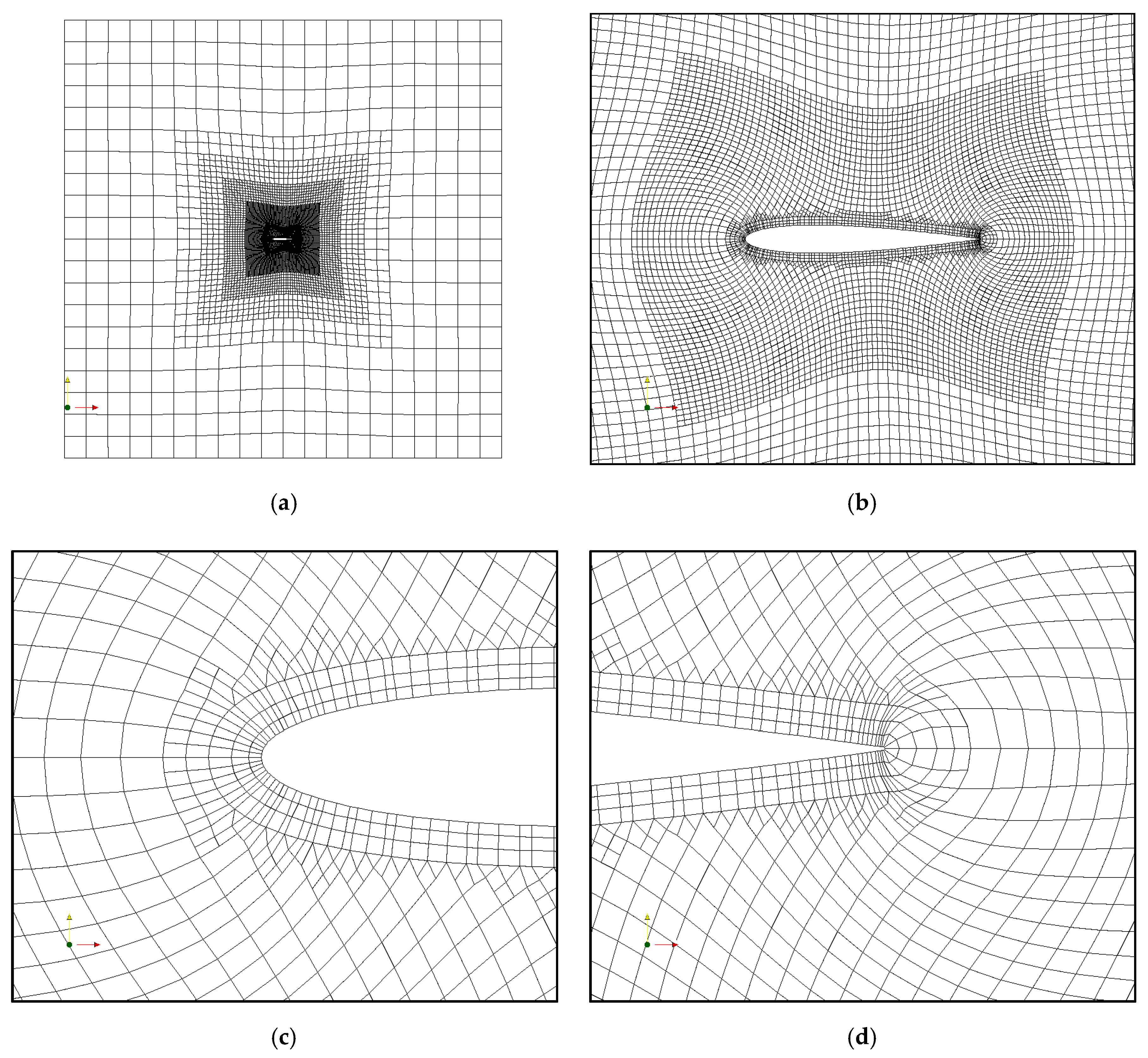
In this section, the RBF and IDW methods are introduced and compared. In addition, an improved RBF method to remedy its shortcomings is proposed. A mesh for a circular cylinder was deformed to the mesh of NACA 0012 using the RBF, IDW, and proposed methods. The red points in Figure 2 denote the control points on the surface of the circle and the blue ones indicate the displaced points on the surface of NACA 0012. The number of control points is 256 and the points move only in the vertical direction. The vertical movements make the normal vectors of the boundary faces rotate.

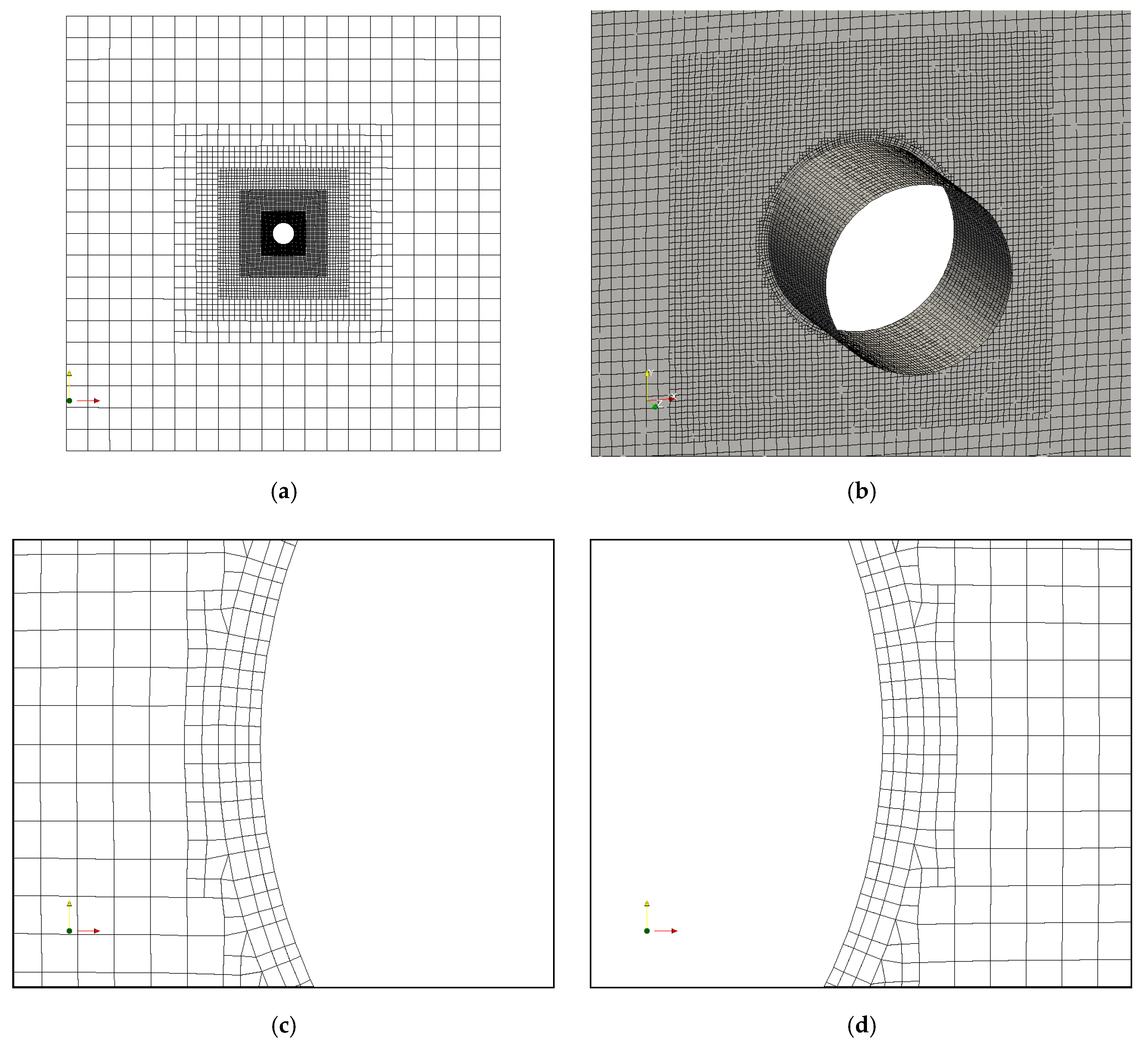
The initial grid for the circular cylinder is shown in Figure 3. The grid is a polyhedral mesh generated using snappyHexMesh, a standard built-in utility of OpenFOAM (The OpenFOAM Foundation Ltd., London, U.K.). The number of cells is 103,160 and the thickness of first boundary layer cell is 1% of the cylinder diameter. The top, bottom, right, and left boundaries were set as fixed boundary conditions. The front and back boundaries were set as symmetric boundary conditions. To satisfy the fixed boundary condition, the grid points of the fixed boundary were added to the control points. The displacements of the fixed boundary were set as zero.

2.1. RBF Method

The RBF method is an interpolation method that uses the distance between the grid point and control points. It was proposed by Sieger et al. [7], Boer et al. [11], Botch and Kobbelt [12], Jakobsson and Amoignon [13], and Michler [14]. The basic formula for displacement is presented in Equation (1).

$$\mathrm{D}\left(\mathrm{x},\mathrm{y},\mathrm{z}\right)={\mathrm{a}}_1+{\mathrm{a}}_2\mathrm{x}+{\mathrm{a}}_3\mathrm{y}+{\mathrm{a}}_4\mathrm{z}+{\displaystyle \sum }{\mathrm{w}}_{\mathrm{i}}\mathrm{U}\left({\mathrm{R}}_{\mathrm{i}}\right)$$

(1)

$${\mathrm{R}}_{\mathrm{i}}=\left|\left({\mathrm{x}}_{\mathrm{i}},{\mathrm{y}}_{\mathrm{i}},{\mathrm{z}}_{\mathrm{i}}\right)-\left(\mathrm{x},\mathrm{y},\mathrm{z}\right)\right|$$

(2)

Here, $R_i$ is the distance between the grid point and the $i$-th control point, and $U$ is a basis function. In this study, a thin plate spline (TPS) is applied as a basis function. The TPS provides a minimal and smooth displacement distribution. The details about basis functions can be found in [15].

$$\mathrm{Thin}\mathrm{plate}\mathrm{spline}:U\left(R\right)={\left|R\right|}^2\log R$$

(3)

The unknowns of Equation (1), $a_i$ and $w_i$, are obtained by calculating Equation (4). The partitioned matrix $K$ is determined by the distance between the control points, and $P$ is composed of coordinates of the control points. Column vector $\overrightarrow{v}$ contains the displacements of control points. Equation (4) is calculated with LU decomposition instead of an iterative method because the matrix is dense and small.

Because the size of the matrix in Equation (4) is proportional to the number of control points, every four points on the fixed boundary is added to the control points. Sheng and Allen [16] applied a greedy data reduction algorithm to reduce the matrix size and calculation time. Coulier and Darve [17] developed the inverse fast multipole method to reduce the computational time. After the mesh deformation, the normal component of displacement of the grid points on the symmetric plane is removed to satisfy the symmetric boundary condition.

$$\left[\begin{array}{cc}K& P\\ P^T& O\end{array}\right]\left[\begin{array}{c}\overrightarrow{w}\\ \overrightarrow{a}\end{array}\right]=\left[\begin{array}{c}\overrightarrow{v}\\ \overrightarrow{o}\end{array}\right]$$

(4)

$$K_{ij}=U\left(\left|\left(x_i,y_i,z_i\right)-\left(x_j,y_j,z_j\right)\right|\right)$$

(5)

$$P=\left[\begin{array}{c}\begin{array}{ccc}1& x_1& \begin{array}{cc}{y}_1& z_1\end{array}\\ 1& x_2& \begin{array}{cc}{y}_2& z_2\end{array}\\ ⋮& ⋮& \begin{array}{cc}⋮& ⋮\end{array}\end{array}\\ \begin{array}{ccc}1& x_p& \begin{array}{cc}{y}_p& z_p\end{array}\end{array}\end{array}\right]$$

(6)

$$O=\left[\begin{array}{c}\begin{array}{ccc}0& 0& \begin{array}{cc}0& 0\end{array}\\ 0& 0& \begin{array}{cc}0& 0\end{array}\\ 0& 0& \begin{array}{cc}0& 0\end{array}\end{array}\\ \begin{array}{ccc}0& 0& \begin{array}{cc}0& 0\end{array}\end{array}\end{array}\right]$$

(7)

$$\overrightarrow{w}=\left[\begin{array}{c}{w}_1\\ w_2\\ ⋮\\ w_p\end{array}\right],\overrightarrow{a}=\left[\begin{array}{c}{a}_1\\ a_2\\ a_3\\ a_4\end{array}\right],\overrightarrow{v}=\left[\begin{array}{c}\overrightarrow{D_1}\\ \overrightarrow{D_2}\\ ⋮\\ \overrightarrow{D_p}\end{array}\right],\overrightarrow{o}=\left[\begin{array}{c}0\\ 0\\ 0\\ 0\end{array}\right]$$

(8)

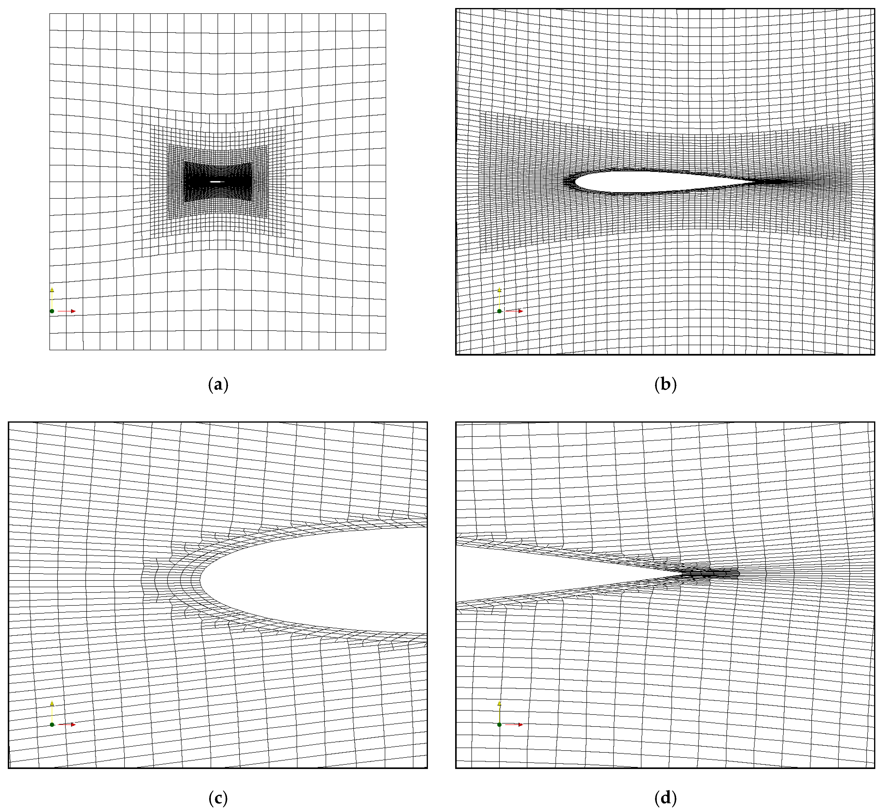
The deformed mesh using the RBF method is illustrated in Figure 4. The overall domain is deformed smoothly, but the boundary layer is thinner than the initial grid and the non-orthogonality is worse than in the initial grid. The maximum skewness and maximum non-orthogonality are compared in

Table 1. Quality of deformed mesh by the RBF method.

	Maximum Skewness	Average Non-Orthogonality	Maximum Non-Orthogonality	Turnaround Time (s)
Initial	0.376	7.233	50.435	-
RBF method	4.742	18.992	86.545	45

. The mesh deformation takes approximately 45 s. The results are similar to those of He et al. [9], who conducted similar mesh deformation using the RBF and IDW methods with a 2D structured grid.

2.2. IDW Method

The IDW method is an interpolation method. The displacement of the grid points is calculated using Equation (9), where $R_i$ denotes the distance as defined in Equation (3). $M_i$ and $T_i$ in Equation (10) are the rotation matrix and translation displacement of the boundary face, respectively. The weighting function is given by Equation (11). Luke et al. [8] suggested these values: $a=3,b=5,\mathrm{and}\alpha =0.25$. $L_{def}$ is recommended as the maximum distance of mesh points, and $A_i$ is the area of the boundary face. In this study, $a$, $b$, and $\alpha$ are set as $3$, $0$, and $0$, respectively. Because of the irregular face area distribution of the boundaries, the thickness of the boundary layer becomes uneven. The calculation time is also reduced since the second term is not calculated.

$$D\left(x,y,z\right)=\frac{{\displaystyle \sum }w\left(R_i\right)s\left(R_i\right)}{{\displaystyle \sum }w\left(R_i\right)}$$

(9)

$$s\left(R_i\right)=M_i{R}_i+T_i-R_i$$

(10)

$$\mathrm{w}\left(R_i\right)=A_i\times \left[{\left(\frac{L_{def}}{R_i}\right)}^a+{\left(\frac{\alpha L_{def}}{R_i}\right)}^b\right]$$

(11)

Figure 5 depicts the deformed mesh using the IDW method. The non-orthogonality of the boundary cell is much better than that by the RBF method. The thickness of the boundary cell is almost equal to that of the initial grid except for the leading and trailing edges. The thickness around the leading and trailing edges is slightly larger than that of the initial grid. The displacements of grid points far from the deformed boundary are smaller than those by the RBF method. The grid quality of deformed mesh is compared with that of the initial grid in

Table 2. Quality of deformed mesh using the IDW method.

	Maximum Skewness	Average Non-Orthogonality	Maximum Non-Orthogonality	Turnaround Time (s)
Initial	0.376	7.233	50.435	-
IDW method	0.571	11.644	73.849	115

. The time for mesh deformation is approximately 115 s, which is ≈2.6 times larger than that by the RBF method.

2.3. Improved RBF Method

The drawback of the RBF method is the non-orthogonality of the boundary layer. To reduce the non-orthogonality, the centroids of the first boundary cells are added as control points. The displacements of the new control points are calculated using the IDW method. To calculate the translational and rotational displacement, the RBF calculation is repeated twice. First, the boundary face is deformed with only the initial control points. The displacements of the centroids of the first boundary cells are calculated with the displacements of the deformed boundary face by the IDW method. Second, the displacements of the volume mesh grid points are calculated with the grid points of the deformed boundary and the centroids of the first boundary cells. To reduce the calculation time, every 4 points of the grid points and centroids is used as control points.

It is difficult to apply both the RBF and IDW methods to problems involving the free surface because the grid around the free surface has to be aligned to the free surface to minimize the numerical diffusion of the volume of fluid function (VOF). Therefore, the deformable region must be limited. The cells around the deformed boundary are designated as deformable cells, while those outside of the regions are set as frozen cells. The faces sheared by the deformable and frozen cells are designated as fixed faces. The points on the fixed faces are added to the fixed control points.

Figure 6 displays the deformed mesh. The non-orthogonality of the boundary cell is better than those by the RBF and IDW methods. The thickness of the boundary cells around the leading and trailing edges is well preserved. The cells in yellow circle are deformable cells.

The quality of the deformed mesh is compared with the initial mesh in

Table 3. Quality of the deformed mesh using the proposed method.

	Maximum Skewness	Average Non-Orthogonality	Maximum Non-Orthogonality	Turnaround Time (s)
Initial	0.376	7.233	50.435	-
Proposed method	0.782	12.141	74.920	13

. The deformed mesh quality using the proposed method is as good as that by the IDW method. Moreover, the proposed method is much faster than the others owing to the limited deformation region.

3. Mesh Deformation for Hull Form Variation

The proposed mesh deformation method was applied to the mesh for ship resistance calculation to examine its applicability to CFD-based optimization. The ship used in the calculations is the JBC model. The scale ratio and the draft are 1:40 and 0.4125 m (16.5 m in full scale), respectively. The speed is 1.179 m/s (14.5 knots in the model).

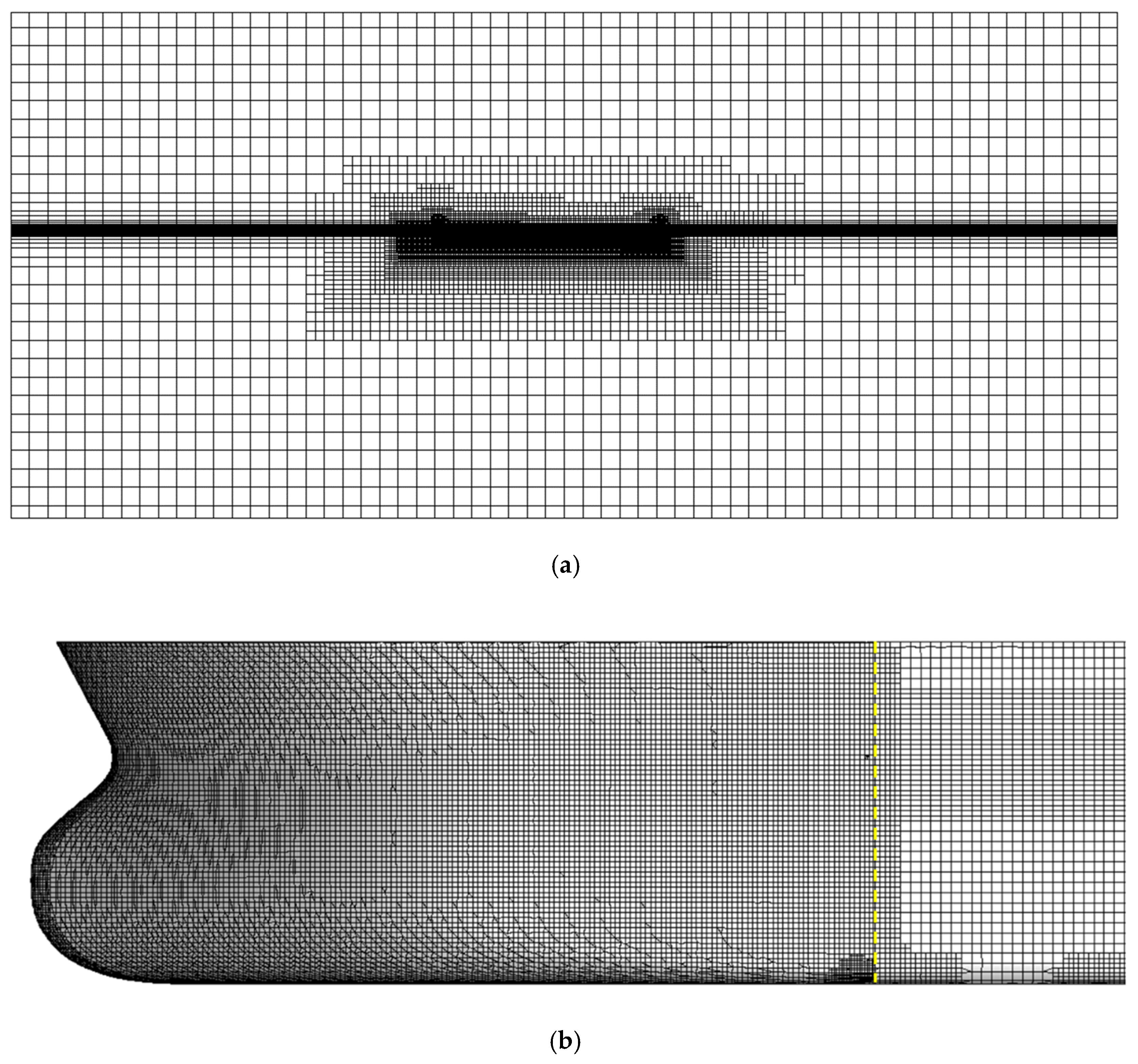
The initial grid used for the JBC resistance calculation is illustrated in Figure 7. The number of cells is 2,402,361. The Y+ of first layer thickness is approximately 50 and the number of boundary layers is 4. The expansion ratio of the boundary layer is approximately 1.3. The running attitude of the ship is fixed as even keel condition. The simulation was conducted using interFoam, a standard solver of OpenFOAM. kOmegaSST and nutUSpaldingWallFunction were used as the turbulence model and wall function, respectively.

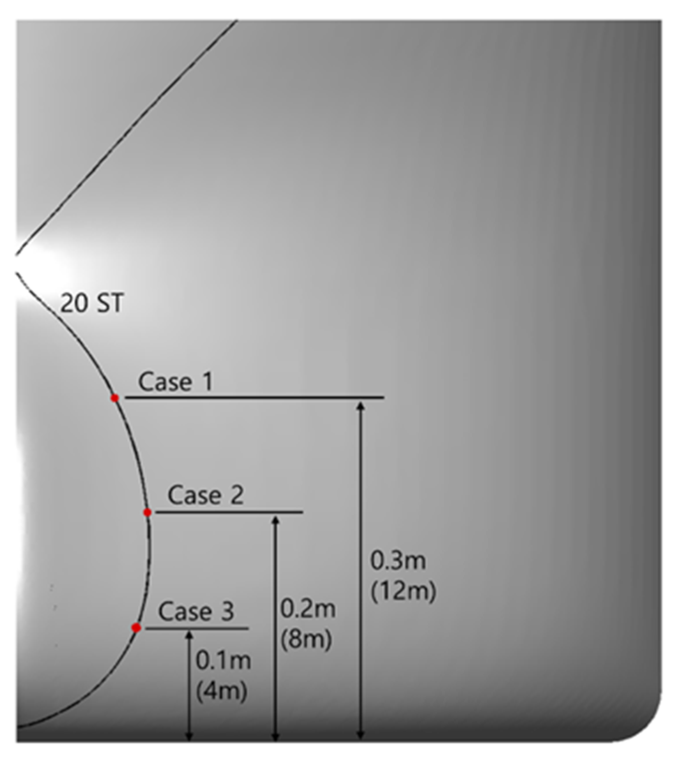
Three points on the forward perpendicular (F.P.) line were moved by 5 mm (0.2 m in full scale) to make an alternative hull form. The hull surface is split by the yellow dashed line in Figure 8. The hull surface in front of the line was set as deformable patch, while that behind the yellow line was set as fixed patch.

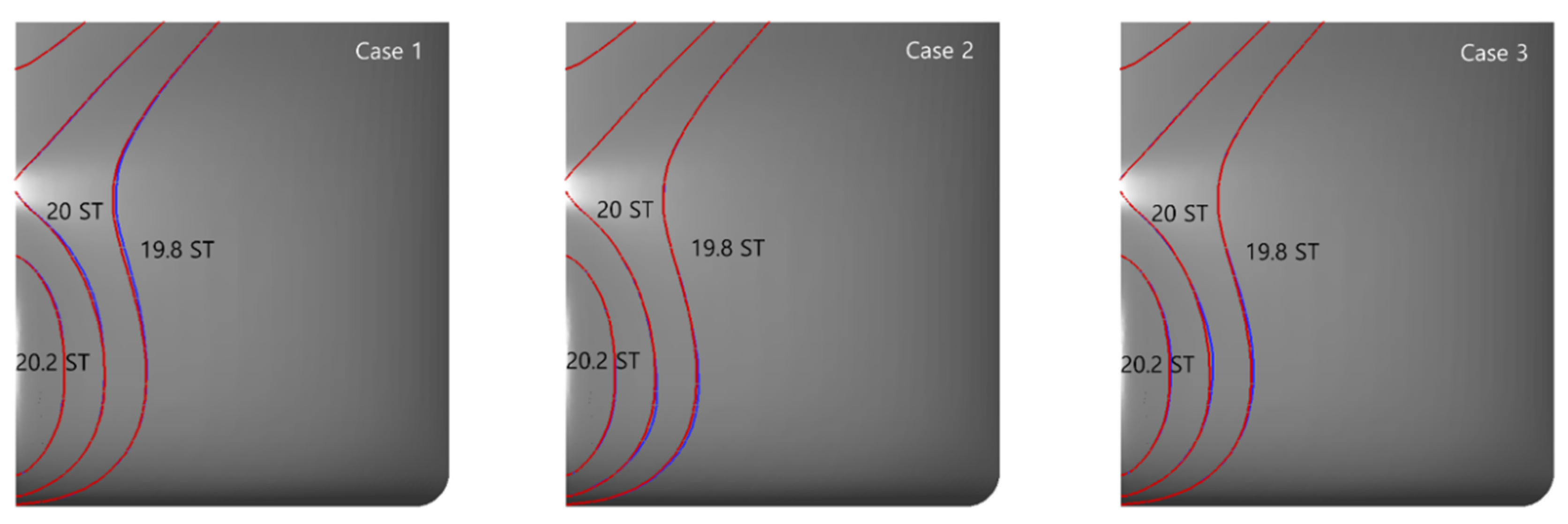
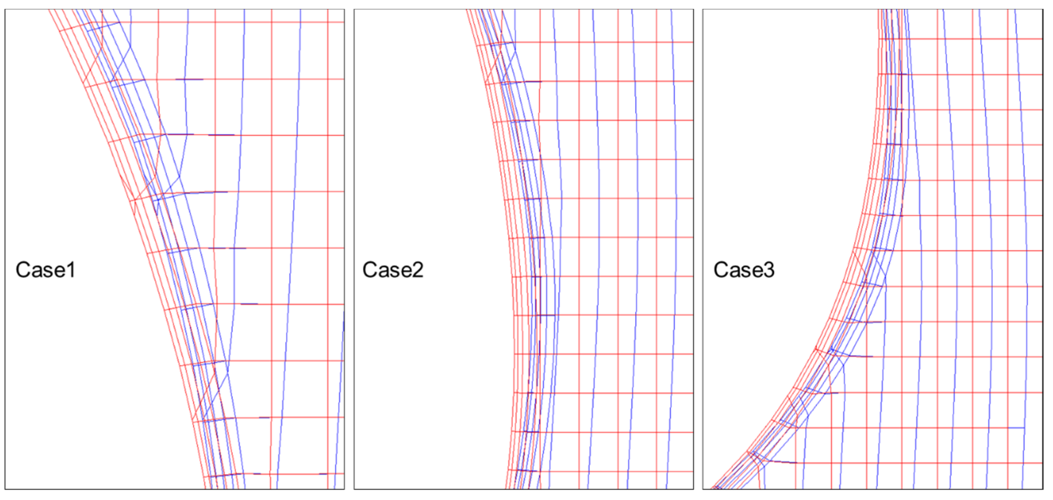
The deformed hull is depicted in Figure 9. The red lines indicate the JBC station lines, whereas the blue lines denote the station lines of the deformed hull. Figure 10 displays a slice of the deformed mesh on the F.P. Because of the small deformation, the variation in mesh quality is small enough to be ignored. The time to deform a mesh with 2 million cells is approximately 118–120 s with a core of Intel Xeon CPU E5-2630 v3 2.4 GHz. The turnaround time is reasonably small. The mesh deformations and CFD simulations are conducted by shell script.

The resistance histories of the JBC and deformed hulls are compared in Figure 11. The calculations of deformed hulls converged much faster than the JBC calculation because the result of the JBC calculation was used as the initial condition for the deformed hull resistance calculations. The calculation of the JBC resistance took approximately 60 s, whereas the calculation of deformed hulls took 20 s in flow time. The variations in the resistances are small because the hull form variation is small. The resistance coefficients are compared in

Table 4. Comparison of resistances of the JBC and deformed hull.

	JBC	Case 1	Case 2	Case 3
Resistance coefficient	4.186 × 10−3	4.187 × 10−3	4.184 × 10−3	4.186 × 10−3

.

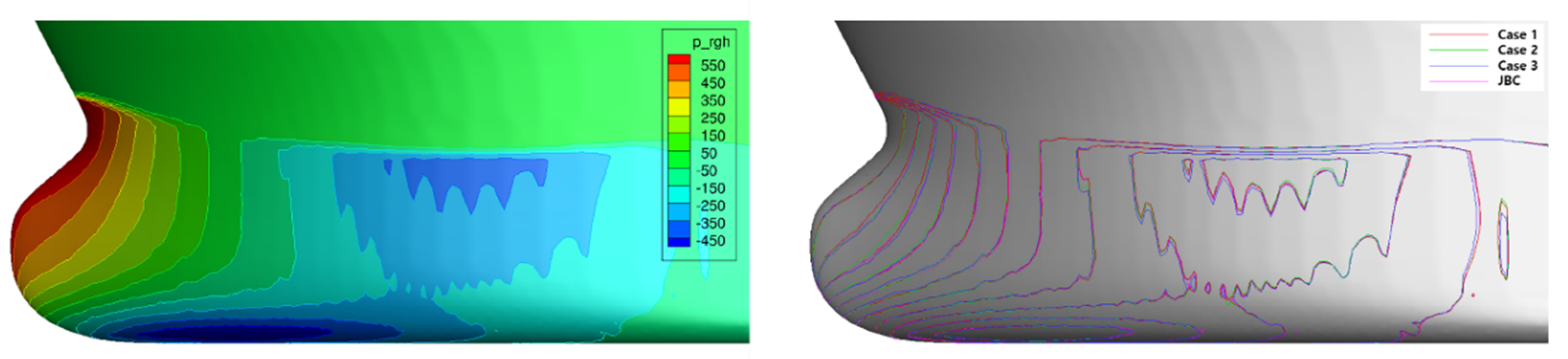
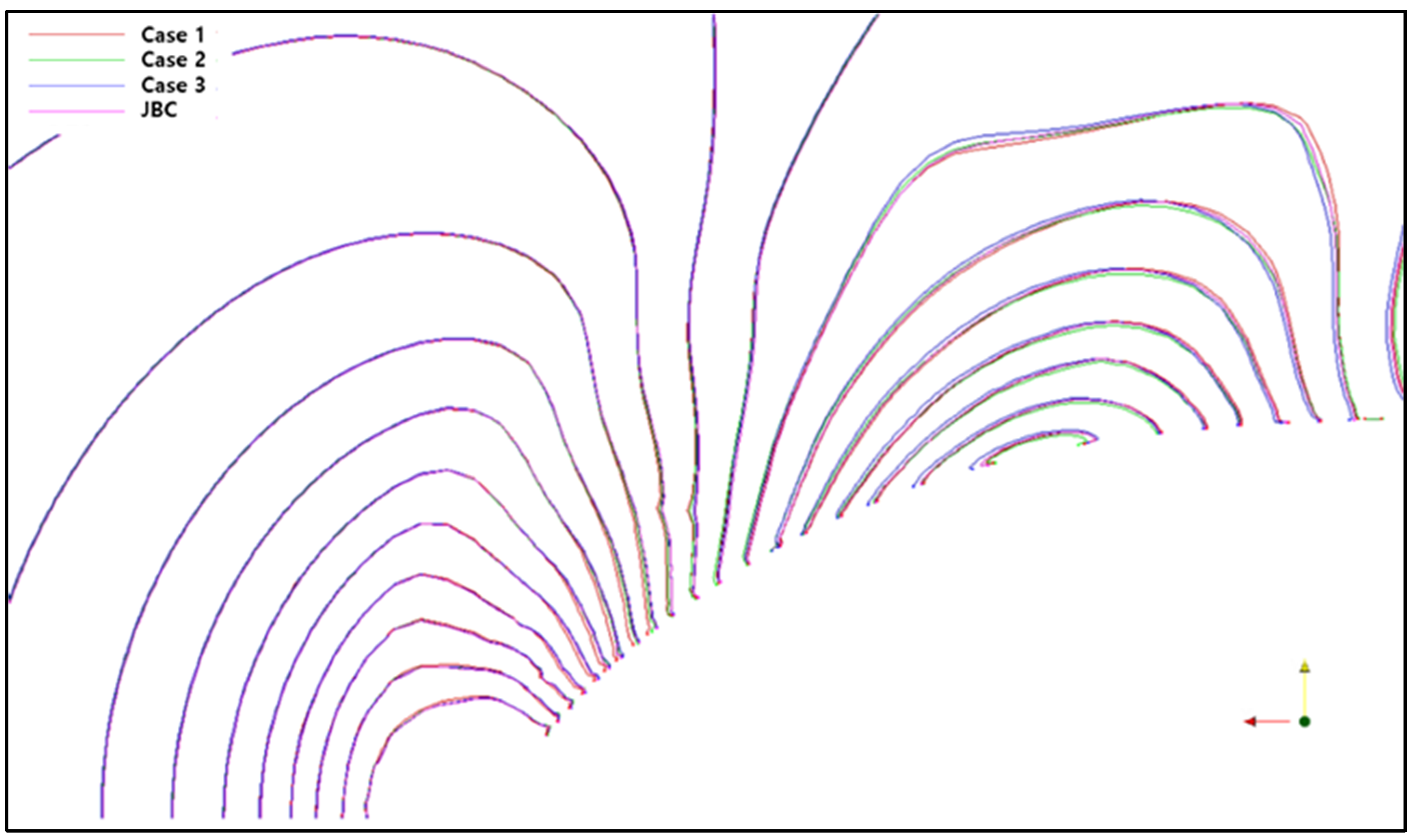
The pressure distributions and wave height contours are compared in Figure 12 and Figure 13, respectively. It was found that the result of the initial hull form can be used as the initial condition for the deformed hull resistance calculation.

4. Conclusions

In this study, two methods for mesh deformation, namely, the RBF and IDW methods, were compared. Moreover, an improved RBF method was proposed for a largely deformed mesh. The RBF method was much faster than the IDW method, but the quality of the deformed mesh using the IDW method was better than that by the RBF method. The quality of the deformed mesh by the RBF method was improved by adding the centroids of boundary cells to the control points. The displacements of the centroids were calculated using the IDW method. The deformable region was limited for the problem involving the free surface. The limitation also reduced the calculation time.

The improved RBF method was applied to the mesh for the JBC resistance calculation to validate its applicability. The resistance was calculated by varying the bow shape with three control points. It took approximately 120 s for the mesh to deform, which is short enough to apply to practical problems. The calculation result of the initial hull form was used as the initial condition for the deformed hull form, which reduced the calculation time to approximately one-third of that of the initial hull form. Thus, the improved RBF method proposed in this study is effective and efficient for hull form variation.

In the future, the CFD-based hull form optimization will be conducted using the proposed mesh deformation method together with an optimization algorithm such as sequential quadratic programming or an adjoint variable method.