Numerical Prediction of the Vertical Responses of Planing Hulls in Regular Head Waves

Abstract

The evaluation of the hydrodynamic performance of planing vessels has always been one of the most attractive study fields in the maritime agenda. Resistance and self-propulsion studies have been performed using experimental and numerical methods by researchers for a long time. As opposed to this, the seakeeping performance of planing hulls is assessed with 2D approximation methods, but limitedly, while the experimental campaign is not cost-effective for several reasons. With this motivation, pitch and heave transfer functions and accelerations were obtained for a monohedral hull and a warped hull using a state of art commercial Reynolds-averaged Navier–Stokes (RANS) solver, in this study. Moreover, 2-DOF (degree of freedom) dynamic fluid–body interaction (DFBI) equations were solved in a coupled manner with an overset mesh algorithm, to find the instantaneous motion of the body. After verification, obtained numerical results at three different Froude numbers and a sufficiently large wave frequency range were compared with the experiments. The results showed that the employed RANS method offers a very accurate prediction of vertical motions and accelerations for planing hulls.

1. Introduction

Planing hulls have been widely used recently for commercial and military purposes in the naval architecture sector. Therefore, hydrodynamic calculations of planing hulls, in terms of resistance, seakeeping, and maneuvering, have become an important issue for marine applications. As is well known, the hydrodynamic investigation of planing hulls is relatively tougher compared to displacement type ships, due to several complex phenomena which are primarily caused by large motions of the body inside fluids. That is the main reason that the very first studies in this field were experimental and remained limited.

As a contribution to the experimental methods, the pioneered study was performed by Savitsky to discover the underlying physics in the planing regime [1]. He proposed an empirical approach that predicts the dynamic trim and total resistance of prismatic hull forms with a very simple algorithm. Several studies have been carried out after Savitsky’s work. The most known experimental study was conducted by Fridsma [2], that covers the behaviors of the prismatic hull forms in both calm water and regular head waves. This study, especially the seakeeping part, is still accepted as a milestone benchmark case for researchers.

As the recent literature is reviewed, there are still many experimental studies carried out in order to explore planing hull hydrodynamics. For example, De Luca and Pensa [3] investigated the hydrodynamics of a warped chinned planing hull series, both in calm water and irregular head seas, experimentally [4]. Begovic et al. [5] studied a similar case by conducting model experiments in regular waves for their planing hull series. In another study, the irregular wave conditions of prismatic and warped hull forms were also investigated by Begovic et al. [6], to find the best statistical approach to represent planing hull performance in the random sea. Santoro et al. [7] conducted a study on the prediction of pressure loads on a high speed planing hull with model experiments in regular waves.

Besides experimental studies, 2D methods based on potential flow theory were also developed by researchers, with many reasonable assumptions. The cornerstone research was conducted by Zarnick [8,9], where he proposed a mathematical model that predicts the vertical motions of planing hulls in regular and irregular head waves. This method simplifies the 3D problem into a 2D water entry problem, and then allows one to calculate the pitch and heave motions. Even though this method was proposed for the seakeeping performance of a planing hull, it can be used for calm water analysis with some reasonable assumptions. Akers [10] put forward a non-linear mathematical model based on Zarnick’s theory and validated the results with the experiments of Fridsma [2]. Van Deyzen [11] also developed a mathematical method based on the theory of Zarnick and he implemented the modifications offered by Keuning [12]. Ghadimi et al. [13] developed another mathematical model which is based on Algarin and Tacson’s studies [14,15] for the coupled heave and pitch motions of planing hulls at non-zero heel angle in regular head waves, and they validated the numerical results with the experimental data of several benchmark models. Tavakoli et al. [16] then used a similar method to calculate the hydrodynamic coefficients of a planing hull.

With the recent development in computational capability, CFD (computational fluid dynamics) solvers are widely used for the calculation of viscous flow around ships, including the planing hulls. Several studies revealing the calm water performance of planing vessels based on the Reynolds-averaged Navier–Stokes (RANS) approach have been carried out by researchers [17,18,19,20]. Thanks to this development, not only calm water characteristics, but also the seakeeping performance of the planing hulls, can be investigated by CFD solvers. Fu et al. [21] examined the hydrodynamic characteristics of a planing hull, both in calm water and head waves, numerically. In regular wave analyses, simulation results were in good agreement for the phases of heave and pitch motions, even though the amplitudes were over-predicted. Mousavariaad et al. [22] presented a comprehensive study about the planing hulls. In this study, they investigated the performance of the historical benchmark Fridsma hull in calm water in deep and shallow water conditions, with fixed and free to trim and sinkage cases. Moreover, their simulation conditions include the regular and irregular head waves in deep water. In regular head waves, they validated the simulation results with the available experimental data by transfer functions of heave and pitch motions and phases with a high order of accuracy. Masumi and Nikseresht [23] performed a numerical study to show the effect of finite depth to calm water resistance and added resistance. Although they investigated different head wave cases, they were only interested in the resistance of the planing hull. Judge et al. [24] made a comprehensive study of a high-speed deep-V planing hull form. They conducted model experiments and numerical simulations in both regular and irregular waves, and they focused on the slamming behavior of the planing hull. It is found that the largest slamming occurs in short and steep waves. The authors validated their numerical approach with vertical motions, accelerations and slamming pressures. Azcueta [25], Wang et al. [26] and Ling and Wang [27] utilized computational fluid dynamics approaches, so that the heave and pitch motions of a planing hull in regular head wave can be accurately predicted. Xiaosheng et al. [28,29] conducted numerical studies on the seakeeping performance of a planing vessel in a regular head wave. After validating the numerical results with the experimental data with a good accuracy, they used different designs to reach a better seakeeping performance.

According to recent literature, it might be said that there is still a room for a numerical investigation about the vertical motion prediction of planing vessels. In this study, URANS computations for a monohedral hull and a warped chine hull form were carried out by solving 2DOF dynamic fluid–body interaction (DFBI) equations with a commercial CFD solver (STAR CCM+) for regular head waves. A verification and validation study was carried out for one velocity and wave frequency for the heave motion. The computational domain was discretized using an overset mesh algorithm. Three different Froude number cases were investigated by means of vertical motions (heave and pitch) and acceleration RAOs (response amplitude operator).

The paper is organized as follows: Section 2 depicts the geometric definition of the hull forms and numerical background, covering the solution procedure and the mesh algorithm. Section 3 gives information about the verification and validation processes. Section 4 gives the obtained numerical results with respect to the motion and acceleration RAOs. Finally, the concluding remarks were given in Section 5.

2. Methodology

2.1. Planing Hull Geometries

In this study, two different planing hull models were used for all simulations. One of them is a monohedral hull that has a constant deadrise angle and the other one is a warped hull (called W3 in [5]) whose deadrise angle changes from stern to bow. Both models belong to the study of Begovic et al. [5,30] The main particulars of these models are shown in

Table 1. Main Particulars of Planing Hulls [5,30].

Main Particular	Mono	Warped
LOA (m)	1.900	1.900
B (m)	0.424	0.424
Δ (N)	319.7	318.5
LCG (m)	0.697	0.586
VCG (m)	0.143	0.156
kyy (m)	0.583	0.519
TAP (m)	0.096	0.108
β (deg)	16.70	9.09–35.75
FnB (-)	1.67, 2.26, 2.82

. In Table 1, L_OA denotes the overall length of the model, B denotes the beam and Δ denotes the displacement of the model. LCG and VCG represent the longitudinal and vertical center of gravity, respectively. β, k_yy,T_AP and Fn_B depict the deadrise angle, gyration radius of the pitch motion, draught at the aft peak and the beam Froude number, respectively. Please note that ${\mathrm{Fn}}_{\mathrm{B}}=\frac{\mathrm{V}}{\sqrt{\mathrm{gB}}}$ where V denotes the forward speed, B denotes the breadth of the planing hull and g denotes the gravity constant.

The 2D geometries of the monohedral and warped hull are shown in Figure 1 and Figure 2, respectively. The L/B ratios are the same for both hull forms and equal to 4. The deadrise angle of the warped hull form is varied linearly from transom to 0.8L, while the mono hull has constant deadrise angle. To avoid much spray and allow the transition to planing regime, the bow has been faired. Detailed information about the hull forms can be found in Begovic et al. [30]

2.2. Numerical Setup

2.2.1. Physics Modelling

The numerical analyses were conducted using a commercial CFD software, solving unsteady Reynolds-averaged Navier–Stokes (URANS) equations. The governing equations are the continuity equation and the momentum equations, considering that the flow is incompressible and turbulent. The continuity equation can be given as:

$$\frac{\partial U_i}{\partial x_i}=0$$

(1)

Velocity $U_i$ can be derived as the mean velocity and the fluctuating velocity components, respectively.

$$U_i=\overline{U_i}+u_i{}^{\prime }$$

(2)

The momentum equations can be written in tensor notation and Cartesian coordinates:

$$\frac{\partial U_i}{\partial t}+U_j\frac{\partial \left(U_i\right)}{\partial x_i}=\frac{1}{\rho }\frac{\partial P}{\partial x_i}+\frac{\partial }{\partial x_j}\left[\upsilon \left( \frac{\partial U_i}{\partial x_j}+\frac{\partial U_j}{\partial x_i}\right) \right]-\frac{\partial \overline{u_i^{\prime }{u}_j^{\prime }}}{\partial x_j}$$

(3)

Here, $\rho$ is the fluid density, $U_i$ is the velocity vector, and $P$ is the pressure. The last two terms belong to the viscous stress tensor, while $\upsilon$ is the kinematic viscosity.

The solution procedure was based on a semi-implicit method for pressure-linked equations (SIMPLE) type algorithm. The turbulent flow was modeled using the k-ε turbulence model that is widely used in numerical ship hydrodynamics. Detailed information about this model can be found in Wilcox [31]. The hull was presumed to be free to only the heave and pitch motions. The dynamic fluid–body interaction (DFBI) method was implemented to represent 2-DOF (degree of freedom) motions accurately. With this implementation, the 2-DOF motion of the planing hull can be obtained by solving the linear and angular momentum equations:

$${\displaystyle \sum \overrightarrow{F}}=m\overrightarrow{a}$$

(4)

$${\displaystyle \sum \overrightarrow{M_G}}=I_G\overrightarrow{a_a}+\overrightarrow{\omega }\times I_G\overrightarrow{\omega }$$

(5)

In Equations (4) and (5), $\overrightarrow{F}$ represents the total force, $m$ represents the mass and $\overrightarrow{a}$ represents the linear acceleration. $\overrightarrow{M_G}$, $I_G$, $\overrightarrow{a_a}$ and $\omega$ depict the total moment according to center of gravity, inertial mass moment, angular acceleration and angular speed, respectively.

Two different coordinate systems are defined. One of them is the earth fixed coordinate system, while the other one is fixed at the center of gravity of the hull. The fluids (water and air) are considered to flow in the negative x direction. The volume of fluid (VOF) approach [32] was utilized with high-resolution interface capturing (HRIC). The discretization orders and some other properties of the physical model are given in

Table 2. Features of the Physical Modelling.

VOF scheme	Second-order
Convectional discretization	Second-order
Temporal discretization	First-order
Interpolation option	Linear
Iteration per one time-step	10

.

In the present work, the time step size was correlated with the encounter period and defined by considering ITTC [33] recommendations and another relevant study [22]. The time step sizes were calculated as follows:

$$\Delta t=\frac{T_e}{2^8}$$

(6)

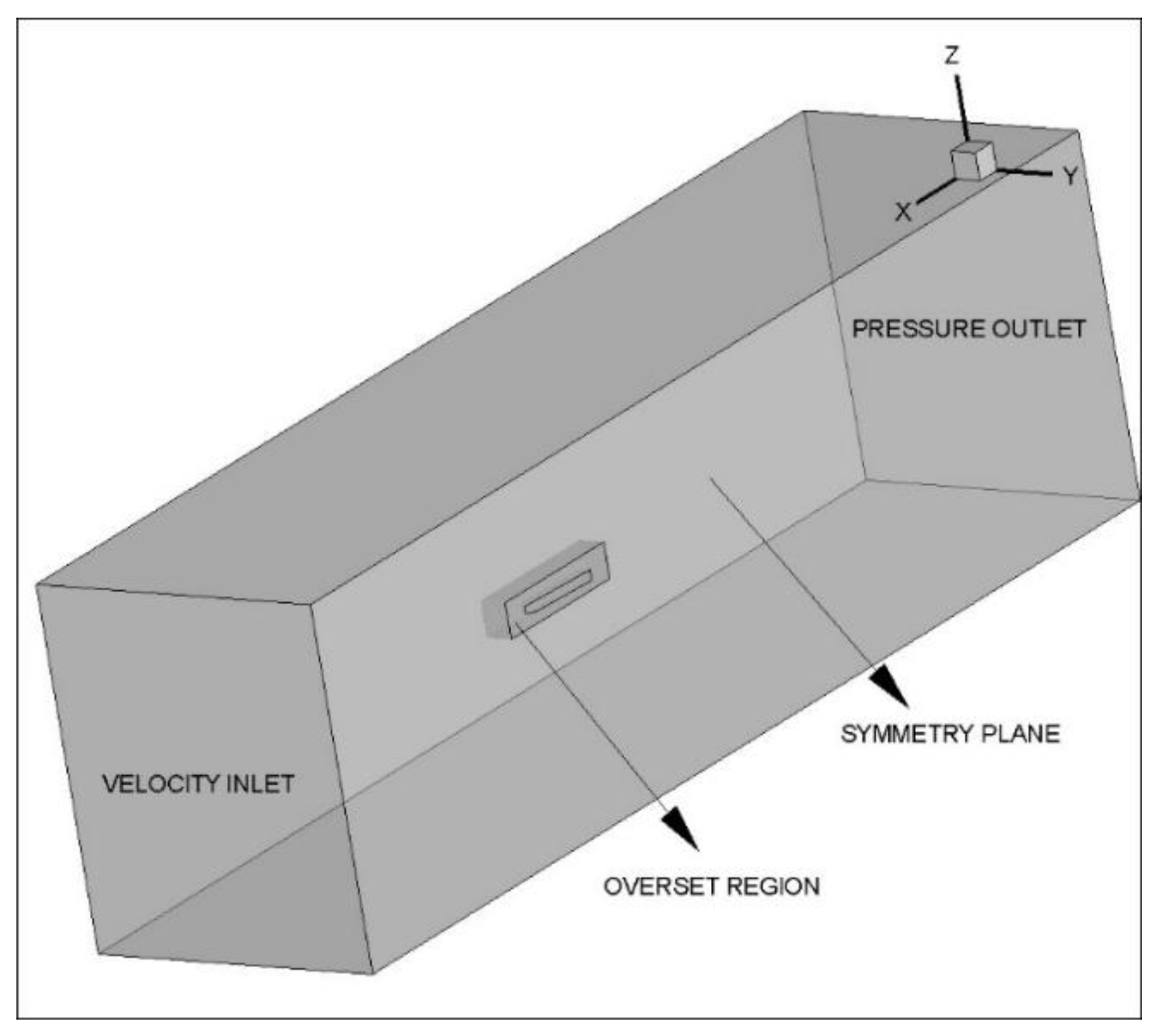
2.2.2. Mesh Generation and Computational Domain

In this study, two different planing hulls were investigated numerically, to obtain the seakeeping performance in regular head waves. The computational domain was created to solve the viscous flow around the planing hulls, by taking the ITTC recommendations [33] into account. The computational domain created in the present study is shown in Figure 3. It should be noted that the computational domain and the mesh structure are set as identical, since these two models have the same length.

In Figure 4, the boundary conditions are shown. As can be seen from this figure, the center lines of the model and the computational domain are aligned to be able to represent the symmetrical phenomena using only half of the domain. Therefore, the computational cost was reduced. The plane aligned with the centerline of the model was defined as the symmetry plane and the outlet plane was defined as the pressure outlet, while the other boundaries were set to be velocity inlet. The planing hull surfaces were defined as a no-slip wall to dictate that the normal component of the velocity is zero.

The computational domain was discretized with hexahedral elements, based on the finite volume method. Since the overset mesh technique proved its perfection on high orientation and translation, it was applied to represent the 2-DOF motions correctly. Therefore, two different mesh regions were created with fully hexahedral elements. The first one was the overset mesh region covering the planing hull, and its near region that is free to motion, in order to predict the vertical motions precisely. The second one was the outer region that the rigid mesh is employed. Trimmer mesh algorithm was employed in both overset and rigid mesh regions. Local mesh refinements were made, covering the free surface and Kelvin wave pattern. The prism layer mesh was applied near the hull geometry to model the flow in the near-wall region precisely, while keeping the wall y+ values between 30–300. Overlap refinements were used for good coupling between the overset and rigid mesh regions. The mesh structure and the refinements are given in Figure 5a,b.

3. CFD Verification Study

The verification study can be applied by reducing time-step and/or mesh sizes to show the convergence of the numerical approaches. In other words, it should show that any scalar value of the numeric solution would go a certain value, with an acceptable uncertainty when the mesh and/or time-step size is reduced. In this paper, the GCI (grid convergence index) method was used for this purpose. This method, which is based on Richardson extrapolation [34], is proposed firstly by Roache [35] and modified by numerous studies [36,37,38]. The methodology presented by Celik et al. [39] was used to determine uncertainty with this technique, as numerous hydrodynamic studies from self-propulsion of submarines [40] to vertical motions of vessels [41].

Before starting the verification study, three different mesh and time-step sizes were determined with a constant refinement factor (r), which was selected as$\surd 2$. After finishing all the analyses, the difference between any scalar values of the solutions can be calculated as follows:

$${\epsilon }_{21}=x_2-x_1 {\epsilon }_{32}=x_3-x_2$$

(7)

Here, $x_1$, $x_2$ and $x_3$ refer to the value of any scalar of fine, medium and coarse time-step or grid sizes, respectively. The convergence condition, which is the ratio of the difference between the solutions, has to be between 0 and 1 to have a monotonic convergence regime. It can be calculated as follows:

$$R=\frac{{\epsilon }_{21}}{{\epsilon }_{32}}$$

(8)

It also should be kept in mind that when a source of uncertainty (time step or mesh) is refined, the other one was kept constant and fine.

In

Table 3. Uncertainty Studies for Heave Transfer Functions (ωe = 7.59_Mono_V = 3.4m/s).

Parameter	Grid Spacing	Time Step
R	$\surd 2$	$\surd 2$
X1 (Fine)	1.080	1.109
X2(Medium)	1.114	1.080
X3 (Coarse)	1.184	1.022
R	0.49	0.51
GCI FINE	3.90%	3.42%

, the uncertainties of the time step and grid size are in an applicable level. It should be kept in mind that, this mesh structure and time step size can be used for the other cases. It also should be noted that, since the relative difference between fine and medium time step size is around 2.5%, the medium time step size (T_e/2⁸) is selected for all simulations similar to Mousavariaad et al. [22].

4. Seakeeping Analyses

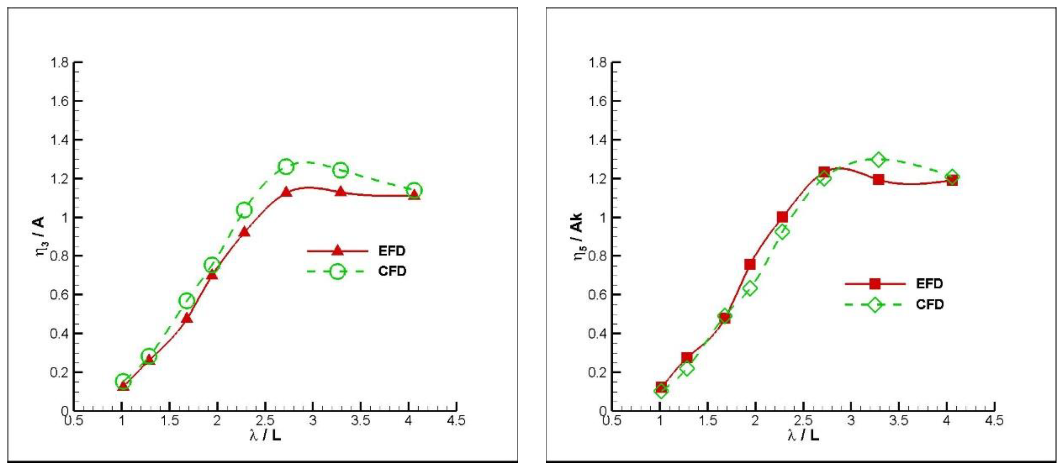
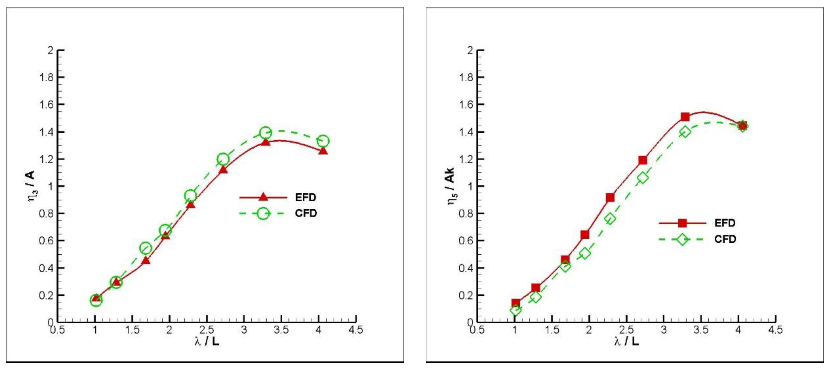
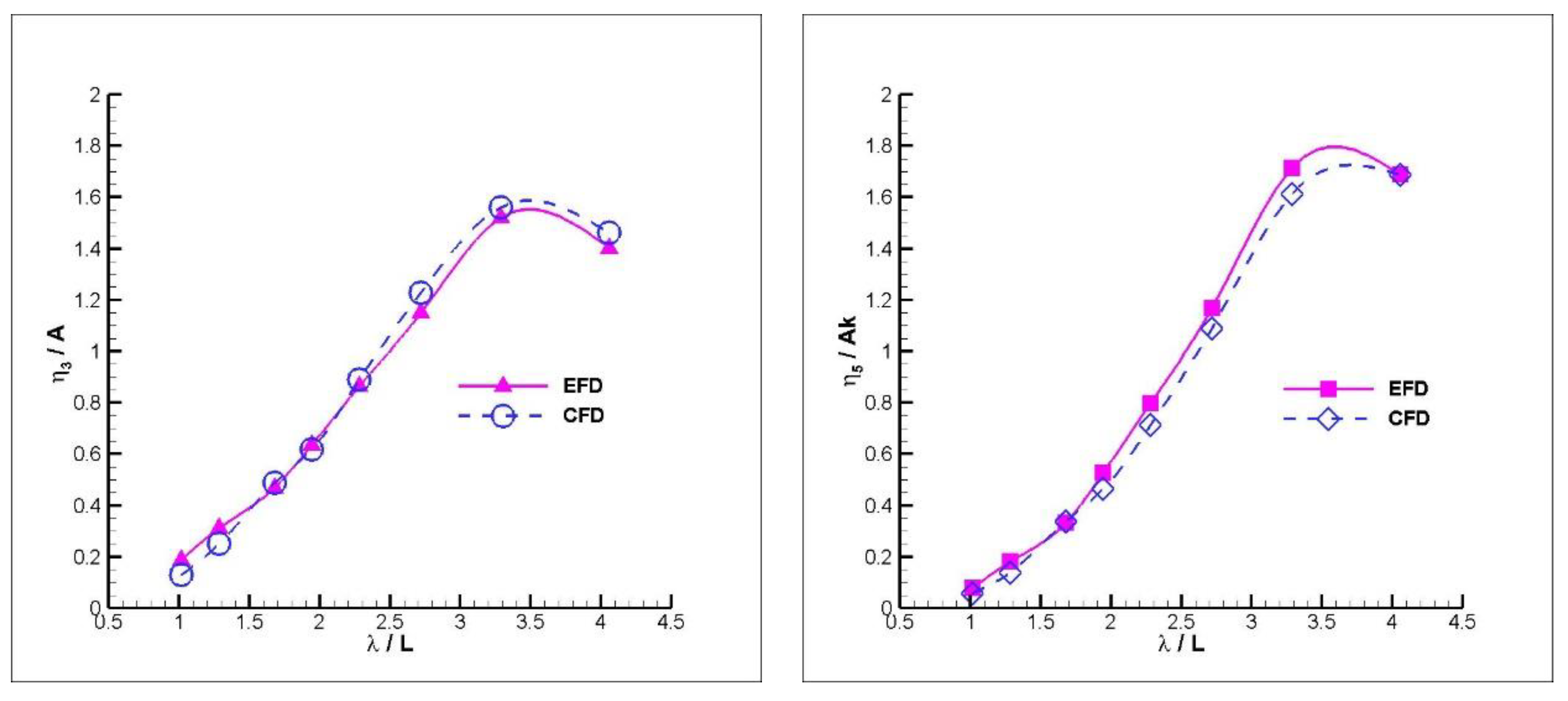
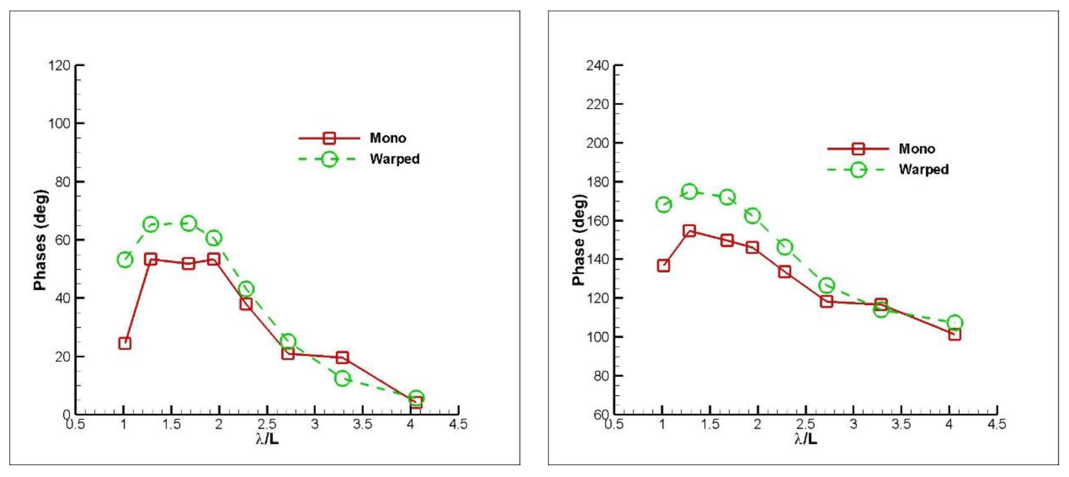
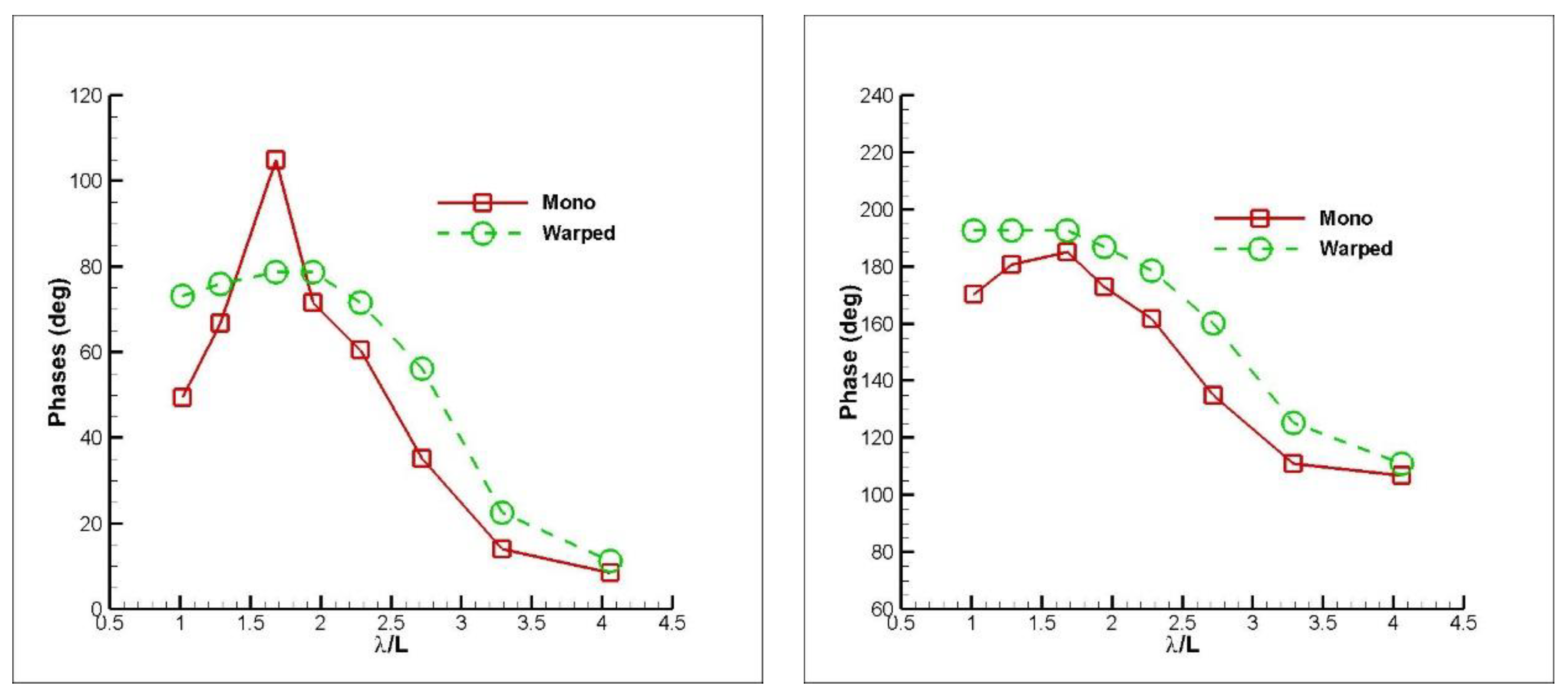
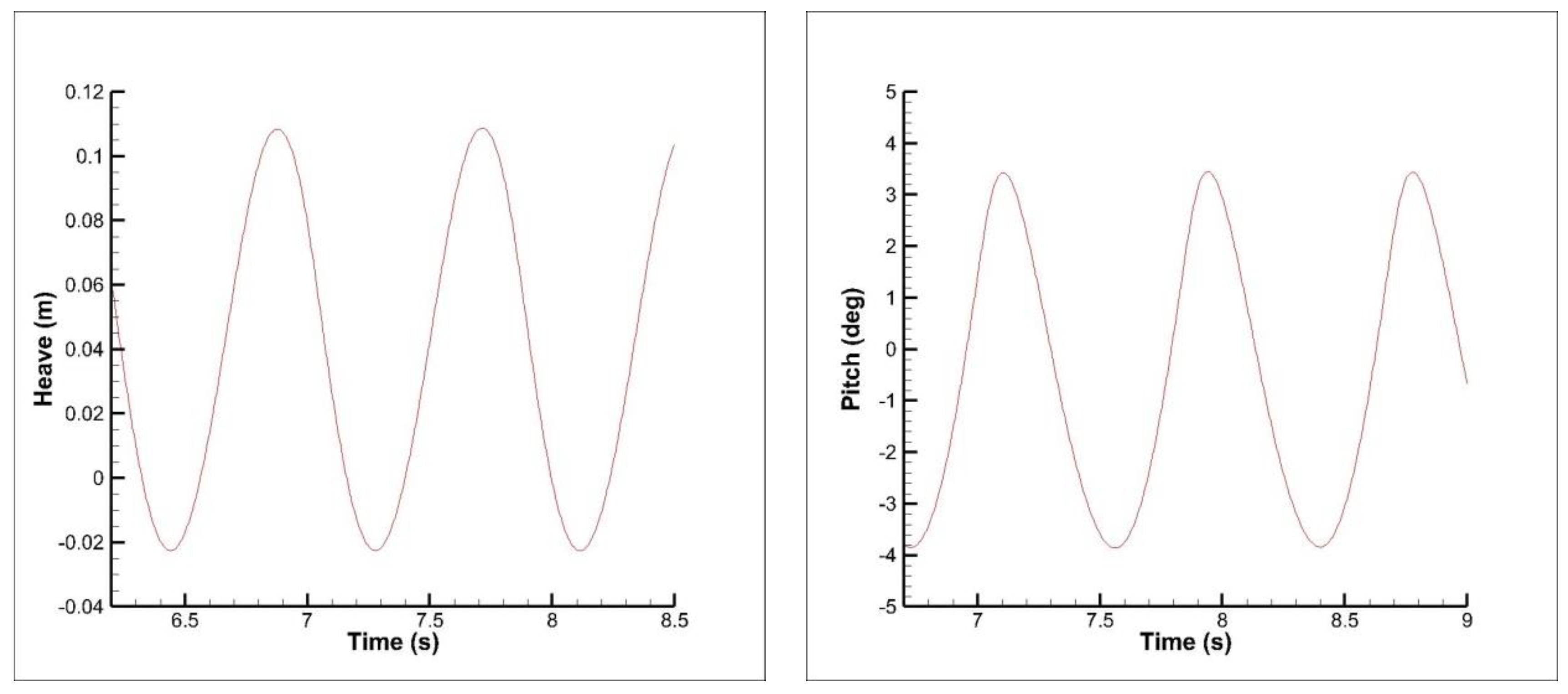
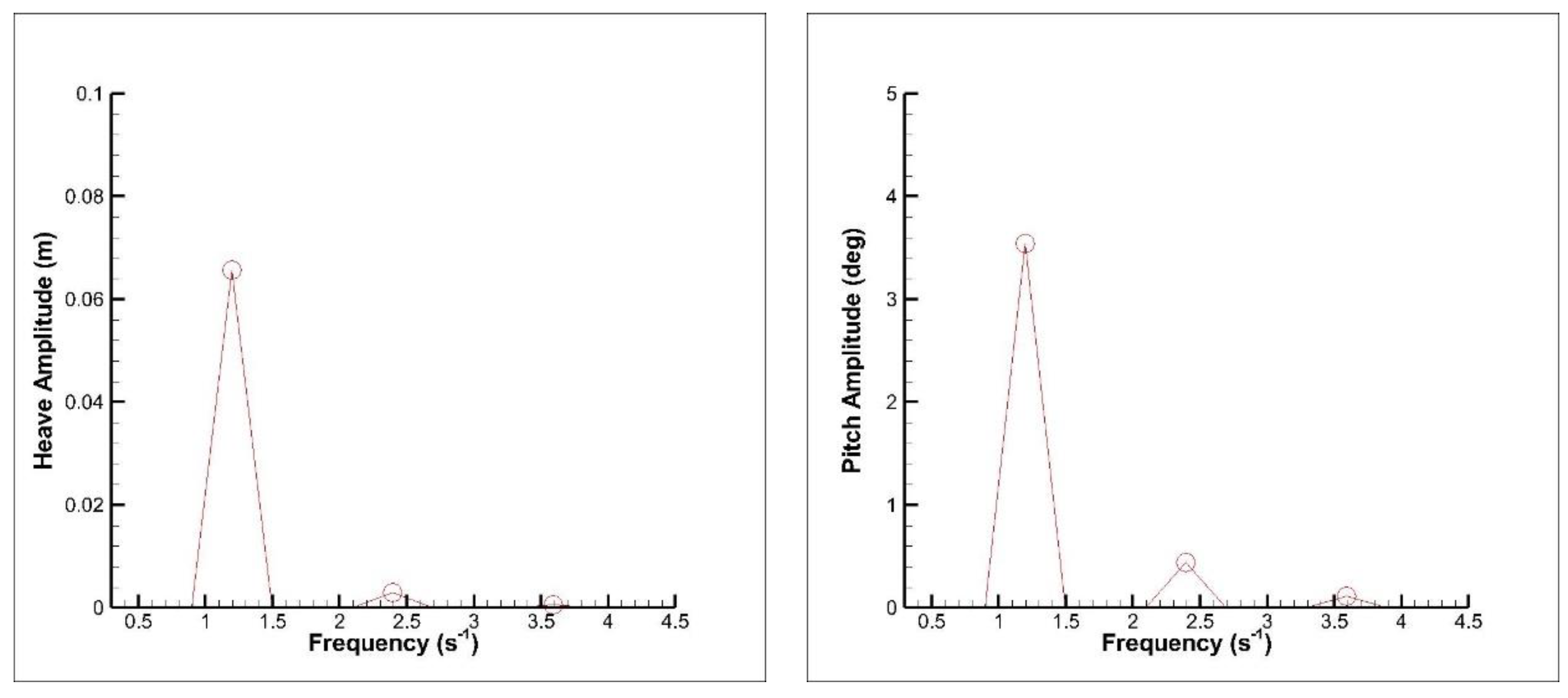
The seakeeping analyses are conducted for two different planing hull models, three different advance velocities and wide-range wave frequencies. The numerical cases are selected identically with the experimental ones [5], to ensure a reasonable comparison. It should be reported that the all numerical analyses took approximately 8–10 h of wall clock time in a 30-core processor with 128 GB RAM for five periods of simulations for each case.

The seakeeping analyses are conducted with the numerical cases listed in

Table 4. Validation Study of Transfer Functions for the Selected Case.

Models	FnB (-)	Case Code	ω (rad/s)	k (rad/m)	λ (m)	A (m)	λ/L
Mono and Warped	1.67 2.26 2.82	C1	5.65	3.260	1.928	0.020	1.014
		C2	5.03	2.576	2.440	0.020	1.284
		C3	4.40	1.972	3.186	0.020	1.677
		C4	4.08	1.700	3.695	0.032	1.945
		C5	3.77	1.449	4.337	0.032	2.283
		C6	3.46	1.217	5.161	0.035	2.717
		C7	3.14	1.006	6.245	0.035	3.287
		C8	2.83	0.815	7.710	0.045	4.058

. The cases are named starting from C1 to C8. It has to be reminded that these cases are repeated for each Fn_B, and for each model, it means that the number of total case is 2 × 3 × 8 = 48.

After observing a steady-state regime for each defined case, the time histories of heave and pitch motions are exported from the RANS solver, to be represented with sinusoidal curves. As there is a need to calculate the first harmonics (amplitude) of the motion for RAO, the trigonometric Fourier series expansion can be used. All the characteristics of a sinusoidal curve can be calculated as follows:

$$\begin{array}{l}{\eta }_i(t)={\eta }_{i,0}+{\displaystyle {\displaystyle \sum }_{n=1}^N}{\eta }_{i,n}\cos (\omega t+{\beta }_{i,n}) \\ n=1,2,3\dots .. i=3,5\end{array}$$

(9)

$$a_{i,1}=\frac{2}{T}{\displaystyle {\displaystyle \underset{0}{\overset{T}{\int }}}{\eta }_i(t)}\sin (\omega t)dt$$

(10)

$$b_{i,1}=\frac{2}{T}{\displaystyle {\displaystyle \underset{0}{\overset{T}{\int }}}{\eta }_i(t)}\cos (\omega t)dt$$

(11)

$${\eta }_{i,1}=\sqrt{a_{i,1}^2+b_{i,1}^2}$$

(12)

$${\beta }_{i,1}=\arctan \left(\frac{a_{i,1}}{b_{i,1}}\right)$$

(13)

Here, ${\eta }_{i,0}$ depicts the zeroth harmonic of the selected signal (heave or pitch), $a_{i,1}$ and $b_{i,1}$ depict the Euler coefficients; ${\eta }_{i,1}$ depicts the first harmonics of the selected motion, while ${\beta }_{i,1}$ depicts the phase angle. Since the motion can be represented by a single frequency that is encountered, the first harmonic of the motion signal is symbolized as ${\eta }_i$ instead of ${\eta }_{i,1}$ for the simplicity. It should be noted that EFD (experimental fluid dynamics) represents the experimental results in all graphs.

4.1. Motion RAOs

In this subsection, the numerical results are compared with the available experimental data, in terms of RAOs of heave and pitch motions. The non-dimensional RAOs of vertical motions are indicated as follows:

$${\mathrm{RAO}}_3=\frac{{\eta }_3}{\mathrm{A}}$$

(14)

$${\mathrm{RAO}}_5=\frac{{\eta }_5}{\mathrm{Ak}}$$

(15)

where ${\eta }_3$, ${\eta }_5$, $\mathrm{A}$ and $\mathrm{k}$ depict the first harmonics of the heave and pitch motions, wave amplitude and wave number ($2\pi /\lambda$), respectively. Here, $\lambda$ is the wavelength. It should be kept in mind that the wave amplitude (A) and wave number (k) are related to the sea surface state and those are listed in Table 4.

RAO graphs consist of three main regions, which are inertia, damping and hydrostatic dominated. The obtained results are discussed in this section by addressing these regions. The results obtained from the numerical study are given in Figure 6 for the mono hull, where the heave and pitch RAOs are compared with the available experimental data for Fn_B = 1.67. As clearly seen, the results in inertia region are generally in satisfactorily good agreement with experimental data for heave motion. At only one wave frequency, which remains in the hydrostatic region, CFD overestimates the heave motion compared to the experimental data. It is noted that the general trend for pitch motion at Fn_B = 1.67 follows the experimental data.

In Figure 7, a similar comparison is made for Fn_B = 2.26 for the monohedral hull. Similar to lowest Fn_B, the discrepancies from the experimental data increase for the relatively larger wavelengths for the heave motion. Similar comments are valid for the pitch motions for the Fn_B = 2.26 case for the mono hull.

Figure 8 reveals the investigation of RAO at the highest Fn_B case. It can be easily seen that CFD generally overestimates the heave motion while it underestimates the pitch motion. It is obvious that the results obtained from CFD are in satisfactorily good agreement with the available experimental data for both heave and pitch motions, for all advance velocities investigated in this study.

The results obtained from the numerical approach for the warped hull are compared with the experimental data in Figure 9, Figure 10, Figure 11 and Figure 12. In Figure 9, the heave and pitch transfer functions are plotted against the experimental data for the Fn_B = 1.67. For relatively larger wavelength regions, the numerical method overestimates the heave motion expect for the largest wavelength. For the pitch motion, while the results of the numerical method are in good agreement with experiments, it can be concluded that it generally underestimates the pitch motion.

Similar to the mono hull case, it can be easily deduced from Figure 10 that the difference for the heave motion is getting higher for the relatively larger wavelengths for the Fn_B = 2.26 case. For the pitch motion, a better agreement than heave motion can be observed in this case as well.

Figure 11 represents the highest advance velocity case, Fn_B = 2.82. Even though CFD generally overestimates the heave motion, it underestimates the heave motion in the inertia region. However, it underestimates the pitch motion for the entire wavelength range.

For both planing hull types, more or less the same findings are obtained for vertical motions. Generally, CFD overestimates the heave motion, although it rarely underestimates the heave motion in the inertia region. A better agreement is observed for the pitch motion for all the Fn_B cases, although it mostly underestimates the pitch motion. Also, for both planing hull types, the largest deviation is detected in Fn_B = 2.26 case for the heave motion, at the hydrostatic region in particular. Figure 12, Figure 13 and Figure 14 show the phase between the wave position at the fixed global coordinate system and heave and pitch motions for the mono and warped hull. The same trends in phases are observed, more or less, for both advance speeds and hull types.

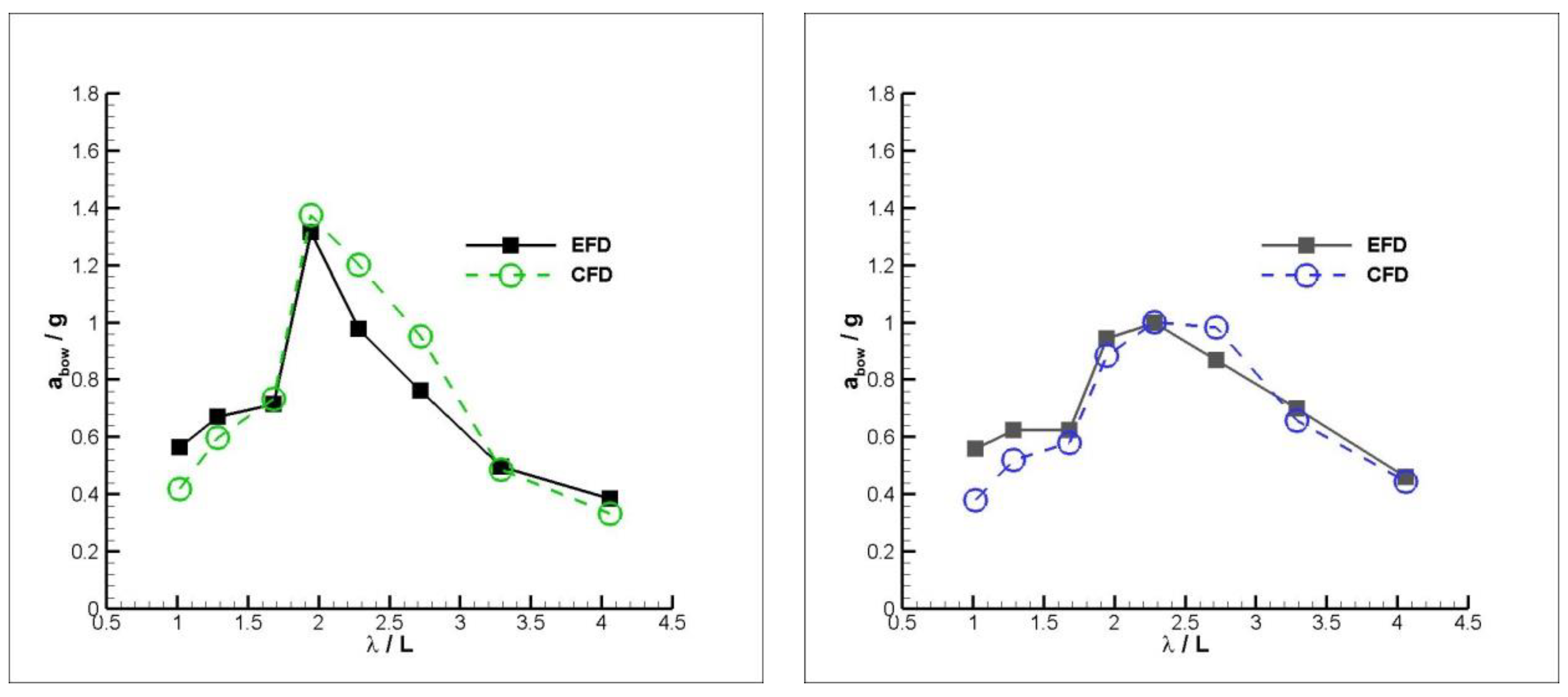
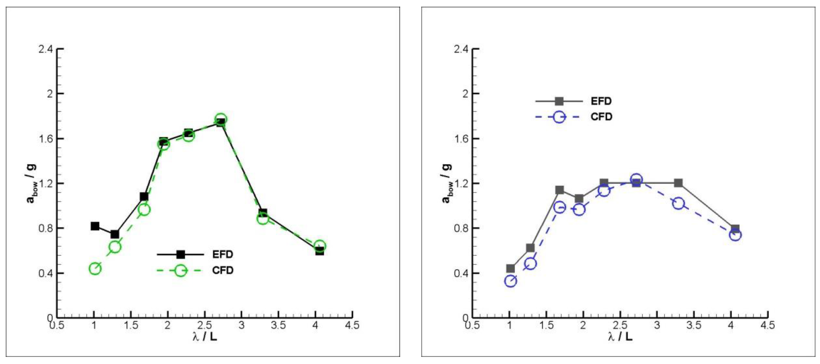
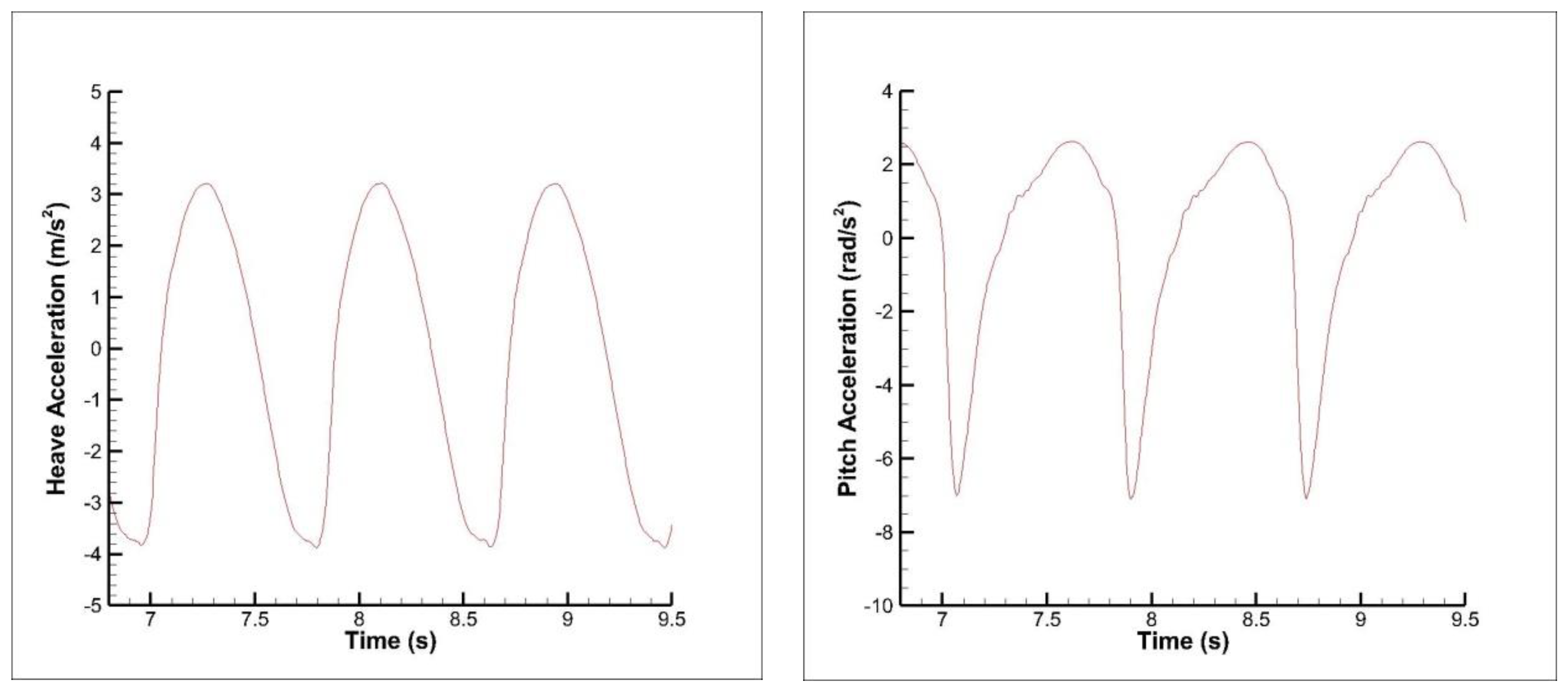
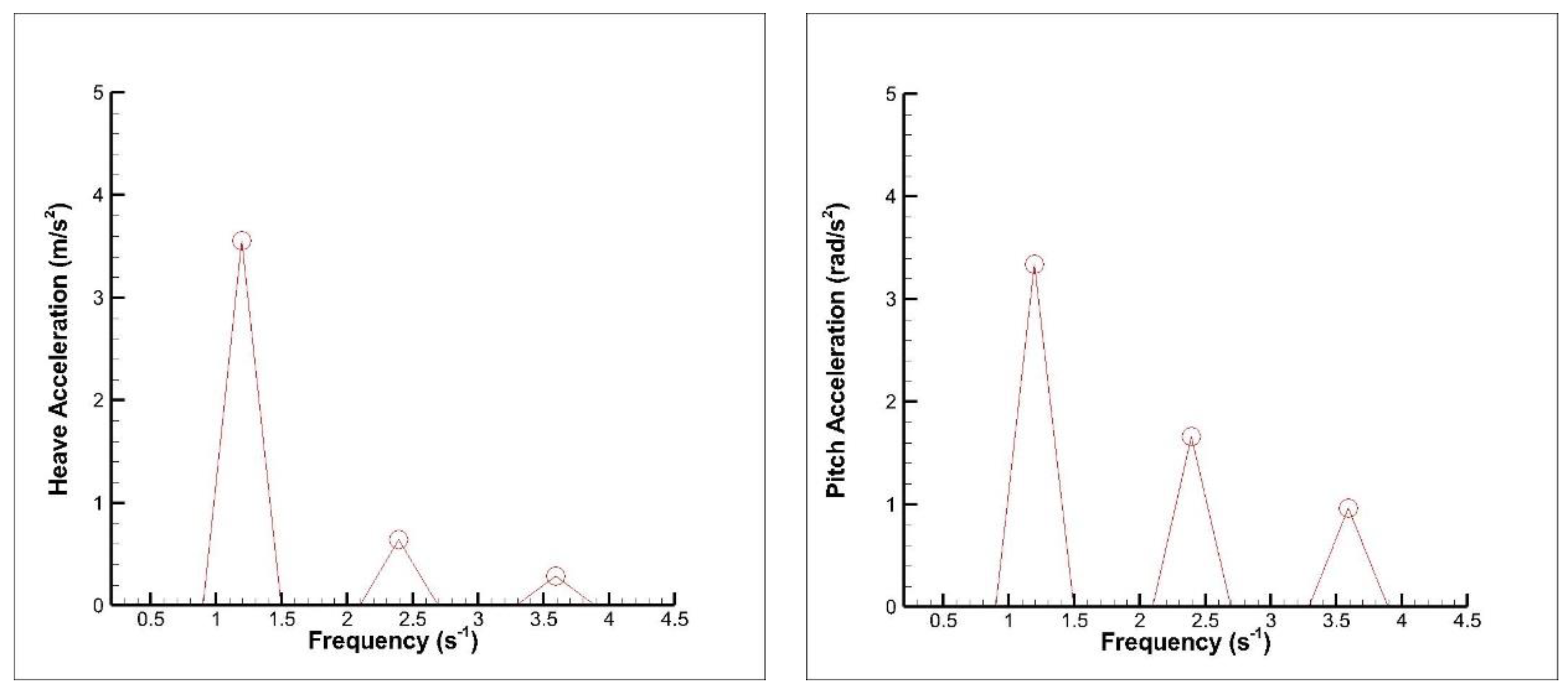
4.2. Acceleration RAOs

After obtaining the time histories of the accelerations at CoG (center of gravity) using CFD, bow accelerations are computed as follows:

$$a_{bow}(t)=a_{CoG, heave}(t)-x_{bow}{a}_{CoG,pitch}(t)$$

(16)

where, $a_{bow}(t)$ denotes the time series of bow accelerations, $a_{CoG, heave}(t)$ and $a_{CoG, pitch}(t)$ denote the time series of heave and pitch accelerations and $x_{bow}$ represents the distance between center of gravity and bow. After reaching the steady state condition, instead of the Fourier series expansion, through to peak analysis, is used for the bow acceleration RAO that is non-dimensionalized by dividing to the gravity constant. The reason of using through to peak analysis is that there is more than one frequency in bow acceleration frequency plot, as opposed to the motion frequency plot that contains reasonable energy. More details will be given below.

The accelerations at bow for both models are shown in Figure 15, Figure 16 and Figure 17. The accelerations at bow are compared for Fn_B = 1.67 for both models in Figure 15. For mono hull, the numerical results are in satisfactorily good agreement with the experimental data. The general tendency of the results for warped hull is quite remarkable with the experimental data, while there are larger deviations than mono hull.

In Figure 16 and Figure 17, the same comparison is made for the higher Froude numbers. In these figures, the general tendency of the bow accelerations is similar with the experiments, although there are some differences for mono hull. However, the tendency is not similar for warped hull, even though the differences are not remarkably high, except for Fn_B = 2.82, λ/L = 1.677 case.

As is seen in Equation (16), the bow acceleration signal is composed of two signals: heave and pitch accelerations. The time histories of heave and pitch motions and their frequency domain response for the case C8 for Fn_B = 2.82 for the warped hull are given in Figure 18 and Figure 19 as an example. As it is drawn from these figures, the only and dominant frequency for heave and pitch motions is the encounter frequency. Therefore, there is only one apparent peak in frequency domain response. It means that RAO can be easily calculated using Equations (9)–(15).

On the other hand, the time histories of heave and pitch accelerations and their frequency domain responses for the same case are given in Figure 20 and Figure 21. As is deduced from these figures, the heave and pitch acceleration signals do not consist of only encounter frequency; there are also other peaks. Therefore, through to peak analysis is used during the calculation of bow RAO.

5. Conclusions

Vertical motions of two different planing hull types under regular head waves are obtained using a commercial RANS solver in the present paper. After conducting a reliable verification study, the analyses are carried out at a sufficiently large frequency range and three different forward speeds. In accordance with the obtained results, the following comments can be made:

• An employed viscous solver is reliable in predicting heave and pitch motions in regular waves and bow accelerations for each case.
• In general, the heave motion is overestimated, while the pitch motion is underestimated at almost all frequencies and advance velocities for both hull forms.
• The deviations between the numerical and experimental results are getting larger with the increase in the wavelength, especially for the heave motion.
• The largest deviations are observed in the minimum wavelength cases (Case 1), for both models at all advance velocities. Since the motions are reasonably smaller in the inertia region, these deviations might be directly related to the measurement difficulties in the experiments.
• Similar to the experiments, more than one dominant frequency is observed in the accelerations. Therefore, the comparison of acceleration RAOs is made with through to peak analysis.
• Since there is more than one dominant frequency in the acceleration signal, the RAO calculation technique might cause a small variation in these results.

As a planned further work, the investigation of irregular wave characteristics for planing vessels will be carried out by the authors.

References

1. Savitsky, D. Hydrodynamic Design of Planing Hulls. Mar. Technol. SNAME News 1964, 1, 71–95. [Google Scholar]
2. Fridsma, G. A Systematic Study of the Rough-Water Performance of Planing Boats; Stevens Inst of Tech Hoboken NJ Davidson Lab.: Hoboken, NJ, USA, 1969. [Google Scholar]
3. De Luca, F.; Pensa, C. The Naples warped hard chine hulls systematic series. Ocean Eng. 2017, 139, 205–236. [Google Scholar] [CrossRef] [Green Version]
4. De Luca, F.; Pensa, C. The Naples Systematic Series—Second part: Irregular waves, seakeeping in head sea. Ocean Eng. 2019, 194, 106620. [Google Scholar] [CrossRef]
5. Begovic, E.; Bertorello, C.; Pennino, S. Experimental seakeeping assessment of a warped planing hull model series. Ocean Eng. 2014, 83, 1–15. [Google Scholar] [CrossRef]
6. Begovic, E.; Bertorello, C.; Pennino, S.; Piscopo, V.; Scamardella, A. Statistical analysis of planing hull motions and accelerations in irregular head sea. Ocean Eng. 2016, 112, 253–264. [Google Scholar] [CrossRef]
7. Santoro, N.; Begovic, E.; Bertorello, C.; Bove, A.; De Rosa, S.; Franco, F. Experimental Study of the Hydrodynamic Loads on High Speed Planing Craft. Procedia Eng. 2014, 88, 186–193. [Google Scholar] [CrossRef] [Green Version]
8. Zarnick, E.E. A Nonlinear Mathematical Model of Motions of a Planing Boat in Regular Waves; David W Taylor Naval Ship Research and Development Center Bethesda Md Dtnsrdc-78/032, USA. 1978. Available online: https://apps.dtic.mil/docs/citations/ADA052039 (accessed on 18 March 2020).
9. Zarnick, E.E. A Nonlinear Mathematical Model of Motions of a Planing Boat in Irregular Waves; David W Taylor Naval Ship Research and Development Center Bethesda Md, Dtnsrdc/Spd-0867-91, USA. 1979. Available online: https://apps.dtic.mil/docs/citations/ADA052039 (accessed on 18 March 2020).
10. Akers, R.H. Dynamic Analysis of Planing Hulls in the Vertical Plane; Meeting of New England Section of SNAME. 1999, p. 19. Available online: https://d1wqtxts1xzle7.cloudfront.net/32221394/nes42999.pdf?1383459146=&response-content-disposition=inline%3B+filename%3DDynamic_Analysis_of_Planing_Hulls_in_the.pdf&Expires=1592664320&Signature=d7eiv564cfspF2x346l1qvXMyEZocxjwSCdcQydINtQAyJd5ISA2eRPai8ANcOt2Q1icLfbIlPmf~dAQFDLMiwzMB4PszT6BUnmzAlk3NR2t0KzKQPKTbV5DSA70UCG4S5hYmu9v75LUxL6g1ihBrjQOFzJ4ortZYnkO3YTIRUMMAdJzKSaeEsEnnmnGKVFC1AUIJ1VYtk~8yrY7~T2t7udCkCIVqhR2USA4J7ZLNdg-06KakhDagZ2CmS5xeL~3o04FX8dMR98I~Hvl6~2q1RCqhVd1Xfkjr-1uOuJvPKiY7Os0r1HsNy4NXfw69dvvdHaO8lLEZuPg2N8Qb9VG1g__&Key-Pair-Id=APKAJLOHF5GGSLRBV4ZA (accessed on 18 March 2020).
11. van Deyzen, A. A Nonlinear Mathematical Model of Motions of a Planing Monohull in Head Seas. In Proceedings of the HIPER08, Naples, Italy, 18–19 September 2008; p. 14. [Google Scholar]
12. Keuning, J.A. Non-Linear Behaviour of Fast Mono-Hulls in Head-Waves. Ph.D. Thesis, Delft University of Technology, Delft, The Netherlands, 1994. [Google Scholar]
13. Ghadimi, P.; Tavakoli, S.; Dashtimanesh, A. Coupled heave and pitch motions of planing hulls at non-zero heel angle. Appl. Ocean Res. 2016, 59, 286–303. [Google Scholar] [CrossRef]
14. Algarín, R.; Tascón, O. Hydrodynamic Modeling of Planing Boats with Asymmetry and Steady Condition. In Proceedings of the 9th Conference on High Sped Marine Vehicles, Naples, Italy, 26–27 May 2011. [Google Scholar]
15. Algarín, R.; Tascón, O. Analysis of Dynamic Stability of Planing Craft on the Vertical Plane. Ship Sci. Technol. 2014, 8, 35–43. [Google Scholar] [CrossRef] [Green Version]
16. Tavakoli, S.; Dashtimanesh, A.; Sahoo, P.K. Prediction of Hydrodynamic Coefficients of Coupled Heave and Pitch Motions of Heeled Planing Boats by Asymmetric 2D+T Theory. In Proceedings of the 37th International Conference on Ocean, Offshore & Arctic Engineering (OMAE2018), Madrid, Spain, 17–22 June 2018; p. V07AT06A009. [Google Scholar] [CrossRef]
17. De Luca, F.; Mancini, S.; Miranda, S.; Pensa, C. An Extended Verification and Validation Study of CFD Simulations for Planing Hulls. J. Ship Res. 2016, 60, 101–118. [Google Scholar] [CrossRef]
18. Mancini, S.; De Luca, F.; Ramolini, A. Towards CFD Guidelines for Planing Hull Simulations Based on the Naples Systematic Series. In Proceedings of the Computational Methods in Marine Engineering VII (Marine 2017), Nantes, France, 15–17 June 2017. [Google Scholar]
19. Sukas, O.F.; Kinaci, O.K.; Cakici, F.; Gokce, M.K. Hydrodynamic assessment of planing hulls using overset grids. Appl. Ocean Res. 2017, 65, 35–46. [Google Scholar] [CrossRef]
20. Judge, C.; Mousaviraad, M.; Stern, F.; Lee, E.; Fullerton, A.; Geiser, J.; Schleicher, C.; Merrill, C.; Weil, C.; Morin, J.; et al. Experiments and CFD of a high-speed deep-V planing hull––Part I: Calm water. Appl. Ocean Res. 2020, 96, 102060. [Google Scholar] [CrossRef]
21. Fu, T.C.; Brucker, K.A.; Mousaviraad, S.M.; Ikeda, C.M.; Lee, E.J.; O’Shea, T.T.; Wang, Z.; Stern, F.; Judge, C.Q. An Assessment of Computational Fluid Dynamics Predictions of the Hydrodynamics of High-Speed Planing Craft in Calm Water and Waves. In Proceedings of the 30th Symposium on Naval Hydrodynamics, Tasmania, Australia, 2–7 November 2014. [Google Scholar]
22. Mousaviraad, S.M.; Wang, Z.; Stern, F. URANS studies of hydrodynamic performance and slamming loads on high-speed planing hulls in calm water and waves for deep and shallow conditions. Appl. Ocean Res. 2015, 51, 222–240. [Google Scholar] [CrossRef] [Green Version]
23. Masumi, Y.; Nikseresht, A.H. 2DOF numerical investigation of a planing vessel in head sea waves in deep and shallow water conditions. Appl. Ocean Res. 2019, 82, 41–51. [Google Scholar] [CrossRef]
24. Judge, C.; Mousaviraad, M.; Stern, F.; Lee, E.; Fullerton, A.; Geiser, J.; Schleicher, C.; Merrill, C.; Weil, C.; Morin, J.; et al. Experiments and CFD of a high-speed deep-V planing hull—Part II: Slamming in waves. Appl. Ocean Res. 2020, 97, 102059. [Google Scholar] [CrossRef]
25. Azcueta, R. Steady and Unsteady RANSE Simulations for Planing Craft. In Proceedings of the 7th Conference on Fast Sea Transportation FAST’03, Ischia, Italy, 7–10 October 2003. [Google Scholar]
26. Wang, S.; Su, Y.; Zhang, X.; Yang, J. RANSE simulation of high-speed planning craft in regular waves. J. Mar. Sci. Appl. 2012, 11, 447–452. [Google Scholar] [CrossRef]
27. Ling, H.; Wang, Z. Numerical prediction and analysis of motion response of high speed planing craft in regular waves. J. Jiangsu Univ. Sci. Technol. Nat. Sci. Ed. 2019, 33, 1–8. [Google Scholar]
28. Bi, X.; Shen, H.; Zhou, J.; Su, Y. Numerical analysis of the influence of fixed hydrofoil installation position on seakeeping of the planing craft. Appl. Ocean Res. 2019, 90, 101863. [Google Scholar] [CrossRef]
29. Bi, X.; Zhuang, J.; Su, Y. Seakeeping Analysis of Planing Craft under Large Wave Height. Water 2020, 12, 1020. [Google Scholar] [CrossRef] [Green Version]
30. Begovic, E.; Bertorello, C. Resistance assessment of warped hull form. Ocean Eng. 2012, 56, 28–42. [Google Scholar] [CrossRef]
31. Wilcox, D.C. Turbulence Modeling for CFD, 3rd ed.; DCW Industries: La Cãnada, CA, USA, 2006. [Google Scholar]
32. Hirt, C.W.; Nichols, B.D. Volume of fluid (VOF) method for the dynamics of free boundaries. J. Comput. Phys. 1981, 39, 201–225. [Google Scholar] [CrossRef]
33. 7.5-03-02-03 Practical Guidelines for Ship CFD Applications. In Proceedings of the ITTC—Recommended Procedures and Guidelines, Copenhagen, Denmark, 31 August–6 September 2014.
34. Richardson, L.F. The Approximate Arithmetical Solution by Finite Differences of Physical Problems Involving Differential Equations, with an Application to the Stresses in a Masonry Dam. Philos. Trans. R. Soc. Lond. 1910, 210, 307–357. [Google Scholar] [CrossRef] [Green Version]
35. Roache, P.J. Verification of Codes and Calculations. AIAA J. 1998, 36, 696–702. [Google Scholar] [CrossRef]
36. Stern, F.; Wilson, R.V.; Coleman, H.W.; Paterson, E.G. Comprehensive Approach to Verification and Validation of CFD Simulations—Part 1: Methodology and Procedures. J. Fluids Eng. 2001, 123, 793–802. [Google Scholar] [CrossRef]
37. Wilson, R.V.; Stern, F.; Coleman, H.W.; Paterson, E.G. Comprehensive Approach to Verification and Validation of CFD Simulations—Part 2: Application for Rans Simulation of a Cargo/Container Ship. J. Fluids Eng. 2001, 123, 803. [Google Scholar] [CrossRef]
38. Stern, F.; Wilson, R.; Shao, J. Quantitative V&V of CFD simulations and certification of CFD codes. Int. J. Numer. Methods Fluids 2006, 50, 1335–1355. [Google Scholar] [CrossRef]
39. Çelik, I.; Ghia, U.; Roache, P.; Fretias, C.J.; Coleman, H.; Raad, P.E. Procedure for Estimation and Reporting of Uncertainty Due to Discretization in CFD Applications. J. Fluids Eng. 2008, 130, 078001. [Google Scholar] [CrossRef] [Green Version]
40. Sezen, S.; Dogrul, A.; Delen, C.; Bal, S. Investigation of self-propulsion of DARPA Suboff by RANS method. Ocean Eng. 2018, 150, 258–271. [Google Scholar] [CrossRef]
41. Tezdogan, T.; Incecik, A.; Turan, O. Full-scale unsteady RANS simulations of vertical ship motions in shallow water. Ocean Eng. 2016, 123, 131–145. [Google Scholar] [CrossRef] [Green Version]
Figure 1. The 2D geometries of the mono hull.
Jmse 08 00455 g001
Figure 2. The 2D geometries of the warped hull.
Jmse 08 00455 g002
Figure 3. Computational domain dimensions.
Jmse 08 00455 g003
Figure 4. Boundary conditions.
Jmse 08 00455 g004
Figure 5. (a) Overset mesh structure around the hull. (b) Local refinements in the domain covering the free surface and the wave pattern.
Jmse 08 00455 g005
Figure 6. Heave (left) and Pitch (right) RAOs of the mono hull at FnB = 1.67.
Jmse 08 00455 g006
Figure 7. Heave (left) and Pitch (right) RAOs of the mono hull at FnB = 2.26.
Jmse 08 00455 g007
Figure 8. Heave (left) and Pitch (right) RAOs of the mono hull at FnB = 2.82.
Jmse 08 00455 g008
Figure 9. Heave (left) and Pitch (right) RAOs of the warped hull at FnB = 1.67.
Jmse 08 00455 g009
Figure 10. Heave (left) and Pitch (right) RAOs of the warped hull at FnB = 2.26.
Jmse 08 00455 g010
Figure 11. Heave (left) and Pitch (right) RAOs of the warped hull at FnB = 2.82.
Jmse 08 00455 g011
Figure 12. Phases of heave (left) and pitch (right) for both models at FnB = 1.67.
Jmse 08 00455 g012
Figure 13. Phases of heave (left) and pitch (right) for both models at FnB = 2.26.
Jmse 08 00455 g013
Figure 14. Phases of heave (left) and pitch (right) for both models at FnB = 2.8.
Jmse 08 00455 g014
Figure 15. Bow accelerations for mono (left) and warped (right) hulls at FnB = 1.67.
Jmse 08 00455 g015
Figure 16. Bow accelerations for mono (left) and warped (right) hulls at FnB = 2.26.
Jmse 08 00455 g016
Figure 17. Bow accelerations for mono (left) and warped (right) hulls at FnB = 2.82.
Jmse 08 00455 g017
Figure 18. Time histories of heave (left) and pitch (right) motions for C7, FnB = 2.26, mono hull.
Jmse 08 00455 g018
Figure 19. Frequency domain response of heave (left) and pitch (right) motions for C8, FnB = 2.82, warped hull.
Jmse 08 00455 g019
Figure 20. Time histories of heave (left) and pitch (right) accelerations for C8, FnB = 2.82, warped hull.
Jmse 08 00455 g020
Figure 21. Frequency domain response of heave (left) and pitch (right) accelerations for C8, FnB = 2.82, warped hull.
Jmse 08 00455 g021