1. Introduction
Whilst high-speed planing hulls have always been of interest to naval architects, substantially less time and resources have been invested into research surrounding the topic than larger, more commercially exploitable areas, such as shipping. In industry, a lot of the knowledge was developed from experience working in the field, and it was commonplace to employ a ‘trial and error’ based design process. Despite this, in recent years there has begun a steady progression in the available work researching high-speed hulls. Notably, in recent years, as is the case across the board with all topics relating to naval architecture, advancements in the power and availability of computational resources have led to an increase in numerical studies using Computational Fluid Dynamics (CFD) to model complex flow.
The use of CFD provides numerous advantages over conventional model testing. Perhaps the most notable of these is the enhanced post processing capabilities and the ability to extract data that is difficult to measure experimentally, such as pressure fields and flow patterns. Before CFD may be used as a design tool with a high level of confidence, it is first necessary to explore its applicability to a given problem, ensuring that it is capable of producing accurate results. While numerous studies have investigated CFD’s capabilities in relation to high-speed vessels, few have looked to determine its ability in modelling the nearfield wake patterns. The nearfield wake region of a planning hull is of specific interest for a number of reasons. Primarily in the case of a planning hull, it may have implications over the choice of propulsion system. There may also be a number or operation specific requirements on the wake produced by a vessel that require analysis of this flow.
A variant of the traditional planning hull that is of particular interest to naval architects is the stepped hull, which aims to minimise the resistance of a vessel through a reduction in the wetted surface area. It has been shown that the inclusion of steps is capable of producing a reduction of 10–15% in the hydrodynamic resistance and typically gives an increase in speed of 6–10 knots [
1]. A stepped hull has one or more transverse discontinuities, or steps, behind each of which the hull elevation raises slightly. When the vessel is travelling at high speeds, air is drawn in through inlets, causing the flow to separate at each step. The forces generated by both the forebody and afterbody must combine to provide vertical equilibrium for a stepped vessel, as well being used to determine the resistance and trim. In order to determine the forces on the afterbody the nearfield wake profile of the forebody must be determined in order to calculate the intersection with the afterbody.
The study reported in this paper sets out to determine the accuracy of CFD in modelling the nearfield longitudinal wake profile through a comparison with physical testing. This will allow designers to use CFD as a tool for the analysis of wake of a planning hull with confidence. In addition to performing this validation, the paper will report on the systematic study of the CFD set up. This will ensure that the most accurate set up is established, as well as highlighting the effects that different set ups have on the accuracy of the simulation. Finally, the work will be used to justify whether CFD is capable of modelling the flow of a stepped hull as it separates from the forebody and interacts with the afterbody of the hull. Modelling the wake profiles without the presence of the afterbody changes the physics of the problem and simplifies it massively; however, it has previously been proposed for the analysis of stepped hulls by Savitsky and Morabito [
2] and provides a good validation case for CFD being able to accurately model flow patterns. This simplification is necessary as experimentally extracting the wake profiles behind a step with anything other than photographs to compare is extremely challenging, and is something that has not been achieved by researchers to date. As such, there is no available validation data for cases where the afterbody is included.
The paper begins by presenting an in-depth literature review of previous numerical studies on the subject of planing hulls. Following this, the aims and the methodology are detailed before the numerical set up is outlined. Finally, the results are presented and discussed, before the work is rounded off with the concluding remarks.
2. Literature Review
There are few examples in literature of authors investigating the near-field longitudinal wake profiles using experimental, analytical or numerical means. A number of studies in the first half of the 20th century attempted to extract the longitudinal wake profiles of planing surfaces [
3,
4,
5,
6]; however, the focus of these studies is upon seaplane floats, and as such, the parameters are vastly different from those typical of planing hulls.
In the past 20 years, some work has been conducted upon the mid and far-field wake of planning hulls. Notably Thornhill et al. [
7] conducted a series of bare hull resistance tests of a planing hull for a range of conditions in order to provide validation data for CFD using an array of capacitance probes. Following this, the same experimental strategy was employed by [
8,
9]. Callander [
8] went on to use the measured experimental data to evaluate the MacPhail 2D + t method for application with planing hulls. His work concluded that the analytical method was able to model the trends of the experimental data; modification was required to improve its accuracy to a suitable level. De Luca [
9] went on to use the data generated to evaluate the effectiveness of interceptors. He provided the profiles he obtained to carry out validation procedures. The experimental procedure followed by these researchers was unable to provide any data for the nearfield wake region due to the placement of the capacitance probes.
Savitsky and Morabito [
2] conducted the first experimental investigation into the nearfield wake of planing hulls, developing empirical equations that quantitatively defined the longitudinal surface wake profiles at both the centreline (CL) and quarterbeam (QB). The authors found that the developed empirical formulae displayed good agreement with the experimental results; however, there is a noticeable scatter and it is clear that while an empirical equation may be capable of providing a good representation of the wake profiles they will not be entirely accurate for all cases. The work undertaken by Stavisky was comprehensive and was published with the intention of aiding the designers of stepped hulls determine how the flow of the fore hull intersects with the aft hull.
The second example of an experimental investigation into the nearfield wake of a planing hull was conducted by Gray-Stephens et al. [
10]. This paper set out to determine the accuracy of the empirical wake equations derived by [
2] when they were employed out with their published range or applicability. The study also examined the accuracy of the Linear Wake Assumption, which is often employed by researchers when modelling stepped hulls in an attempt to evaluate its validity for this application. A further motivation behind this paper was to provide detailed experimental data to be used for the validation of CFD in modelling the flow in this region, as is being undertaken by the present study.
The number of available numerical studies investigating both planing and stepped hulls has been increasing rapidly in recent years. This has led to vast improvements in the level of accuracy that is reported by authors, with a mean prediction error of 10% being considered achievable by the International Towing Tank Conference (ITTC) [
11]. This prediction error is for the calculation of forces and there is little information available to evaluate the accuracy CFD in modelling wake field.
Following a study of the available literature, the authors of this paper were unable to identify any examples of experimental data being used to validate or evaluate the performance of CFD in calculating the longitudinal wake profiles of a high-speed planing hull. A number of studies do however make use of Savitsky’s Wake Equations in conjunction with numerical methods, primarily as one-off validation cases of the CFD. In 2014, Faison [
12] used the Savitsky Wake Equations to compare the wake profiles of transverse steps with the CFD generated profiles of swept back and cambered steps. The study found there to be significant differences between the numerical and empirical profiles however the authors were unable to determine if the differences were solely accountable to the change in design, or due to the superior accuracy of one the methods employed. In 2015 Ghadimi et al. [
13] used the Savitsky Wake Equations to validate a numerical computation modelling the CL wake profile. The authors went on to use the validated simulation to investigate how altering the transom stern may reduce the wakes rooster tail height. The paper shows the validation comparison to have reasonably good correlation, but, once again, the authors are not able to comment on the reasons behind this difference. Moreover, in 2015, Lotfi et al. [
14] compared a numerically generated CL wake profile to the equivalent one calculated using the Savitsky Wake Equations. Similarly to [
12] the two methods are not shown to have good correlation, featuring an average error of 20%. Most recently, in 2017 Bakhtiari and Ghassemi [
15] were investigating the effect of a forward swept step angle on the performance of a planing hull through the use of CFD. They employed the results of the Savitsky Wake Equations as part of their validation procedure, showing that there is a reasonable level of agreement between the two methods, but that they do not exactly agree.
No examples of authors investigating the modelling of the nearfield wake profiles with CFD were found, aside from those using the Savitsky Wake Equations as a brief validation case. Those using the Savitsky Wake Equations to validate their CFD model often found discrepancies between the two methods, however, were not able to identify which of the methods was closer to the physical solution. The lack of investigation into this topic is in part due to the lack of experimental nearfield wake data available in the public domain, with only two sources of this being identified. Some studies have compared mid and far-field experimental wake cuts with CFD results for conventional displacement ships. Analysis of the work submitted to the Gothenburg 2010 Workshop revealed that wave cuts closest to the hull tend to be well predicted; however, as distance from the hull increases, the results varied considerably [
16]. This workshop was for a KCS vessel, and it is well known that CFD is significantly more accurate when evaluating conventional displacement ships compared to planing hulls. An example of this comparison being made for planing hulls was undertaken by Mancini [
17]. The study compared the numerical results for the wake field to the experimental mid and far field wave cuts of the Naples Systematic Series. It was found that CFD was able to model the trends in a satisfactory manner; however, it was noted that there was differences in both the amplitudes and phase of the results.
3. Aims and Objectives
The primary aim of this study is to perform an in-depth investigation into the ability of CFD in modelling the near-field longitudinal wake profiles of a planing hull. An evaluation of both the CL and QB profiles will be made through a comparison with experimental data. Additionally, comments will be made upon the accuracy of CFD in comparison to Savitsky’s Wake Equations and the Linear Wake Assumption. The secondary aim of the work is to investigate how the set-up of a CFD simulation may affect its accuracy, with the most accurate set up being presented in detail. Following this, the findings relating to the influence of a number of factors on the simulation results will be outlined so that their impact may be quantitatively understood. Throughout this study, there is a specific focus on turbulence modelling. In order to achieve these aims a number of objectifies have been identified:
- (1)
develop a CFD simulation that may be considered accurate;
- (2)
systematically investigate the identified factors to establish their influence;
- (3)
perform a Validation and Verification study to ensure a high confidence level in the CFD simulation;
- (4)
quantitatively evaluate the accuracy of CFD at modelling the nearfield longitudinal wake profiles of a planing hull through comparisons of the CL & QB profiles;
- (5)
qualitatively evaluate the accuracy of CFD at modelling the wake pattern of a planing hull through comparison of surface elevation plots with experimental pictures;
- (6)
comment on the set up deemed to be most accurate and make comparisons to other methods.
4. Methodology
The global methodology of the project was broken down into two stages. The experimental work as performed by [
10] was to be used as validation data:
The first stage was to set up a CFD simulation capable of accurately modelling the longitudinal wake profiles. The simulations were tuned to ensure the best set up was achieved, with a number of factors being systematically varied to determine the effects on the predicted wake profile. Once an accurate simulation had been developed, an extensive Validation & Verification (V & V) study was undertaken. All numerical simulations were performed using the commercial software, Star CCM+ (12.04.011-R8), on the University of Strathclyde’s Archie-WeST High Performance Computer.
The second stage was for all cases that were experimentally tested to be run using the CFD simulation, allowing a comparison to be made over a range of conditions. The results were then assessed both quantitatively and qualitatively to provide a detailed assessment of the accuracy of CFD. As the paper [
10] from which the experimental data was obtained also investigated the accuracy of Savitsky’s Wake Equations and the Linear Wake Assumption comments will also be made towards the accuracy of CFD in relation to other methods.
While it is possible to develop a robust and reliable numerical model based on either an overset grid or morphing mesh methodology that is capable of resolving the final attitude of a planing vessel these approaches were not utilised. Instead, the hull was fixed in both sinkage and trim. This methodology was chosen for two key reasons. Firstly, the experimental study had employed a hull that was fixed in sinkage and trim to give the researchers more control over the position for which the wake profile was being extracted, allowing a broad range of cases to be examined. Secondly, it is known that CFD is accurate in modelling the position of a planing vessel that is free to sink and trim, and it was not the place of this study to further evaluate this. In order to ensure an exact comparison between the experimental data and the numerical result and give a fair evaluation of CFDs capabilities it was important that the hull positioning was exactly the same in the experimental and numerical studies. Introducing the typical ~10% error in both sinkage and trim of the CFD simulation through a model that was not fixed would add uncertainty and taint the analysis of the wake profiles.
5. Experimental Set Up
The experimental results were obtained from [
10]. Please refer to this paper for detailed discussion upon the experimental set up. This section will, however, briefly detail the experimental testing that was undertaken.
The experimental work used a simple prismatic hull form, featuring a constant deadrise. It was tested in the fully planing condition in calm water. The lines plan is presented by
Figure 1.
The experimental test matrix was defined to cover a broad a range of hull positions, allowing a robust validation case for the CFD set up across a number of conditions. A total of 175 runs were completed, taking measurements for 12 test cases featuring three trim (
τ) conditions and four speeds. The hull parameters for each test case are detailed in
Table 1, where the draft given is the immersion of the transom once the model has been positioned correctly. Due to the speed limitations of the carriage, a small-scale testing methodology was employed.
The wake profiles was measured using sonic probes mounted on a gantry behind the model, as detailed in
Figure 2. Additionally, the forces and moments were measured to allow further validation of the CFD simulation.
6. Numerical Set Up
This section outlines the approach followed when developing the numerical simulation, giving the specific details of the final set up that was deemed the most appropriate for modelling this problem. Information regarding alternate set ups and the effect of these upon the simulations results is presented in the results section. Detailed information upon the inner numerical workings of the CFD code will not be discussed as the commercial solver Star CCM+ was used, and such details are not relevant to the scope of the work. Detailed information outlining the inner workings of a CFD solver can be found in [
18]. The numerical set up was in the same scale and conditions as reported in the experimental study, ensuring that both the Froude and Reynolds numbers in both were identical.
6.1. Physics Modelling
It is commonplace to use a two-equation turbulence model for numerical studies into ship hydrodynamics, with [
16] stating that they have been proven to give accurate predictions. Whilst more advanced models are available it was found by the ITTC following the analysis of entries to the Gothenburg 2010 Workshop, that there was no visible improvements to the accuracy of a resistance simulation when these are used.
The most widely used two-equation turbulence models for engineering application are κ−ε and κ−ω. Both are used when studying ship hydrodynamics; however, variants of κ−ω are far more prevalent, accounting for 80% of the submissions for the Gothenburg 2010 Workshop. When comparing the models the ITTC concluded that turbulence model selection has little impact upon the accuracy when analysing resistance [
11]. A review of studies investigating planing hull performance through CFD found that there was no clear indication that one was more favourable than the other with both being used in a number of papers:
The κ−ω
SST model is known to be more computationally expensive, with simulations taking up to 25% longer to run [
28]. Despite this downside, studies have shown it to be superior when predicting separating flows and wake patterns [
11,
16]. Additionally, it has been shown to be the most prevalent turbulence model for use with marine hydrodynamics over the past two decades [
29].
An investigation into turbulence model selection revealed that for low planing hull simulations turbulence model choice resulted in a notable variation in the calculated forces and moments. It was also shown to have reliable impact upon the accuracy of the calculated wake program. In this investigation κ−ω SST proved to be the most accurate, so this model was selected despite the fact that it is more computationally expensive.
The Volume of Fluid (VOF) method was used to model and track the position of the free surface. It is known for its numerical efficiency and is a simple-multiphase model that is well suited to simulating flows of immiscible fluids. The model introduces a ‘volume fraction’ variable, which is used to define the spatial distribution of each phase. A cell with a volume fraction of 0.5 contains a 50:50 mixture of air and water, and is used by the VOF method to define the free surface.
A known and documented problem when modelling planing hulls using the VOF method is that it can lead to Numerical Ventilation (NV), or Steaking, which may be considered one of the main sources of error in these numerical simulations [
21,
26] NV occurs when the free surface is not captured adequately and results in air falsely being introduced into the boundary layer flow adjacent to the hull. When NV occurs, it has a negative impact on the calculation of forces as it alters the fluid properties. Gray-Stephens et al. investigated a number of strategies to minimise NV [
30]. All strategies that were found to be effective were employed in the setup of this simulation to ensure that NV did not affect its accuracy. Additionally, over the course of the current work it was found that including a surface tension model equal to 0.072 N/m helped to reduce NV further when used in conjunction with established methods.
The surface tension coefficient expresses how easily two fluids can be mixed, with a higher surface tension represents a stronger resistance to mixture. The coefficient itself is defined as the amount of work necessary to create a unit area of free surface [
31]. For the most part the effects of surface tension are negligible with The ITTC Specialist Committee on Computational Fluid Dynamics stating that they may usually be neglected for ship hydrodynamics problems [
32]. As this work adopted a small-scale testing approach, the surface tension forces are larger relative to the hydrodynamic forces than for a more conventional model size. It was thus necessary to determine if neglecting these forces was valid, or if they must be included in the simulations.
Including the surface tension model had a significant effect upon the forces calculated. This was achieved through a reduction in the level of NV (
Figure 3), which changed the fluid properties in the near wall cells. It has been concluded a number of times that it is not possible to eradicate NV, however it is possible to reduce it to a level that is acceptable for engineering purposes [
31,
33]. This study presents a new viable strategy to reduce the levels of numerical ventilation. This is supported by [
34], who investigated free surface flows with air entrainment and concluded that failure to include the surface tension model resulted in an increased level of air entrainment.
All previous studies investigated planing hull hydrodynamics that were found over the course of the literature review followed a high
approach, using wall functions to model turbulence. A low
approach is desirable if an accurate prediction of the boundary layer velocity is required, for instance in drag calculations, and if the cell count and simulation time is not considered a critical issue [
35]. Adopting a low
approach almost doubled the cell count and increased the computational time required for convergence by a factor of three, however lead to a significant improvement in the accuracy of both the wake profile and forces.
As the cell count and simulation time were not considered critical issues the low approach was selected, primarily due to the improved the accuracy in calculating the wake profiles, however also as it reduced the comparison error in resistance to a more acceptable level. The low approach resolves the viscous sublayer and, as such, the simulation should be more representative of the physical phenomena occurring.
6.2. Timestep
A timestep may be selected to ensure that it satisfies the flow features of interest or that it satisfies the Courant–Friedrichs–Lewy (CFL) condition. For standard pseudo-transient resistance simulations, a timestep that satisfies the flow features of interest is usually selected when an implicit solver is employed. When the V & V study (as presented in
Section 7) was performed, a number of timesteps were tested. The timestep study revealed that as the timestep was reduced by a factor of two, the calculated forces featured Monotonic convergence upon a solution. The average timestep convergence ratio for all forces was 0.27, and was as low as 0.016 for resistance. The selection of timestep was made to balance the computational run time against the accuracy of the solution. It was shown that when the timestep was reduced further there was no significant improvement in the results. A timestep (
) that satisfactorily resolves the flow features as a function of the vessels speed (U) and the wetted length (
of the hull was selected, such that:
It was ensured that the selected timestep was within the range suggested by the ITTC for such simulations in all cases [
36]. Satisfying the CFL condition for all cells resulted in an impractically small timestep that would result in an unjustifiable increase in computational time. It would also have a negligible impact upon the results over a timestep that was selected to ensure that the flow features of interest were satisfied through a timestep independence study. The verification study determined that a timestep defined by Equation (1) is capable of resolving the flow features of interest, suitably balancing accuracy against computational time.
6.3. Computational Domain
It is well documented that for a CFD simulation to be accurate the choice of domain size must be appropriate, such that the boundaries are placed sufficiently far away to ensure they have no effect upon the solution through interaction with the wake. The ITTC recommend that the inlet and exterior boundaries are located 1–2 Length between perpendiculars (
) from the hull, with the outlet being placed 3–5
downstream [
37]. It is also important to ensure that wake does not intersect with the side boundary as this can cause reflections that influence the solution. Due to the narrow wake associated with a planing hull this is of less concern than for a conventional displacement simulation. The sizing of the computational domain was chosen in accordance with ITTC recommendations and may be seen in
Figure 4. To ensure the domain was robust and suitable for all possible trim conditions the overall length of the model was used rather length between perpendiculars, or wetted length.
In addition to selecting an appropriately sized domain, the VOF Wave Damping option was enabled on the side and outlet boundaries to ensure that wave reflections did not impact the solution. The VOF Wave Damping option introduces a vertical resistance to vertical motion, and suppresses waves, and prevent them reflecting back into the simulation. A damping zone of one length overall was chosen.
6.4. Boundary Conditions
The selection of appropriate boundary conditions is essential to ensure that the solution remains accurate whilst at the same time managing the computational costs of the simulation. The Dirichlet boundary condition was applied, simulating free flow. A common practice to reduce the size of the domain for calm water resistance simulations is to implement a symmetry condition on the x-z plane at the centreline of the hull. The nature of the wake profile was shown to include symmetrical elements of flow that crossed the centreline and interact with one another. As such, prior to employing this strategy, tests were undertaken to determine if it influenced the calculated wake profiles. It was shown that there was negligible impact upon the results and, as such, the symmetry boundary condition was utilised, halving the computational demand.
If the simulation were to be an accurate representation of the physical tank, the walls of the domain would be modelled using no-slip walls, the top as an inlet, the front as an inlet, and the rear as a pressure outlet. The modelling of no-slip walls requires the inclusion of a prism layer mesh, and this in turn requires volume mesh refinements to ensure the interface between the volume mesh and the prism layer mesh is appropriate, maintaining an acceptable volume change between cells. Such a selection of boundary conditions is impractical due to the significant increase in cells. A simplification to avoid this is to model the sides and bottom of the domain as inlets. The inlet condition is reported to be the least computationally expensive, whilst the selection of any appropriate combination of boundary conditions has no significant affect upon the flow results, provided they are located suitably far from the vessels hull [
28]. The physical tank walls were far enough from the hull as to have no influence upon it, while the depth was great enough to consider the scenario a deep-water problem. Similarly, the domain of the simulation is large enough that the boundaries are far enough away to have no impact upon the result.
Extra consideration was given to the deep-water assumption. Before employing this assumption for the CFD case, the following were checked for the experimental test regime:
6.5. Computational Grid
A planing hull is subject to larger variations in trim and sinkage than a conventional displacement hull. One of the greatest challenges when developing a numerical simulation modelling a planing hull is ensuring the mesh can accurately deal with these motions. For this test program, the physical model was fixed in sinkage and trim, removing the need for the mesh to be capable of modelling motion and allowing a rigid mesh to be used as opposed to morphing or overset grids.
To generate the mesh Star CCM+’s automated meshing capability was utilised [
35], with the surface remesher, automatic surface repair, trimmed cell c and prism layer mesher selected. The ‘trimmed cell mesher’ was selected as it aligns the cells with the direction of the flow, minimising numerical diffusion. This feature relies upon the Cartesian cut-cell method. It allows for a large degree of control through the use of local surface and volumetric controls that allow the user to increase or decrease the mesh density. This method presents a robust and efficient method of producing a high-quality grid, predominantly made up of unstructured hexahedral cells with polyhedral cells next to the surface. The mesh is formed by constructing a template mesh from the target sizes input by the user, and then trimming as required, this using the input surfaces. Using a trimmer mesh enables the use of growth parameters that can be used to ensure there is smooth transitions within the mesh and help prevent the introduction of numerical errors.
Volumetric controls were used to progressively refine areas of the mesh in which flow features of interest occurred, ensuring that the mesh was capable of capturing the complex flow in these regions. The areas that were identified for progressive refinement were the free surface, the area surrounding the hull, and the wake region, with three layers of increasing refinement used for each. Additional refinements were included at the bow, the stern, and for the free surface upstream of hull. These further enhance the resolution where the largest flow gradients occurred, and to help prevent Numerical Ventilation.
Figure 5 shows the computational grid and the refinements that it contains. It should be noted that the mesh shown was for the coarsest studied in the mesh study as it shows the refinement zones clearly.
To allow the simulation to accurately resolve the high velocity gradients associated with the boundary layer flow the ‘prism layer mesher’ was used. This generates orthogonal prismatic cells adjacent to the hull. These are high-aspect ratio cells that are aligned with the local flow and are vital for the accuracy of the simulation. The thickness of the prism layer was calculated to be equal to the thickness of turbulent flow (
) for a given Reynolds number (
over a flat plate of the same wetted length (
, as calculated by [
40]:
After the simulation converged satisfactorily, a scalar plot of the Turbulent Viscosity Ratio was checked to ensure that the prism layer was thick enough. If the prism layer mesh is not thick enough then a non-trivial amount of turbulent viscosity would be present in the core mesh, indicating that part of the boundary layer has diffused into the core mesh region.
The first cell height of the prism layer was calculated to ensure that the
value was below one. A stretching ratio of 1.2 as suggested by [
37] was used to grow the prism layer until it reached the desired thickness. Care was taken to ensure that the outer layer of the prism layer mesh and the first layer of the core mesh were of comparable sizes to ensure that numerical errors were not introduced.
An additional volumetric refinement was included in the area in which the free surface met the hull. The prism layer thickness was reduced to 25% of the calculated thickness in this region as suggested in [
30].This further reduces Numerical Ventilation as it decreases the numerical diffusion caused by the cells of the prism layer that are misaligned with the free surface.
A mesh study was undertaken to ensure that the mesh was fine enough, resulting in the final mesh consisting of around 20 million cells. The choice to follow a low approach significantly increased the cell count, however as the body was fixed this did not result in an impractical computational time to reach convergence. Simulations took between 7.5–27 h to run on the Archie-WeST High Performance Computer (HPC), equating to between 300–1080 core hours. The large variation in run time was caused by differences in the physical time the simulation had to run for to converge satisfactorily. Another factor effecting the run time was that some simulations required very large number of iterations in the early stages of the simulation to ensure that the large gradients associated with beginning a simulation did not cause divergence.
7. Verification and Validation of CFD
In most examples of planing hull simulations available in literature validation is conducted by a straightforward comparison of the simulated result and tank testing data. This approach is rather basic and may not be used to evaluate the true accuracy of the simulation. It is possible for numerical and experimental results to be very close; however, this may be by chance with the simulation containing considerable numerical uncertainties, which combine to give the correct result. Without conducting a thorough Verification and Validation (V & V) study, there can be little confidence in any results as the accuracy and uncertainty of the simulation has not been evaluated. As such, one should be completed prior to generating any results for analysis. The ITTC has published guidelines on how best to perform a V & V study in relation to marine simulations [
41]. The full V & V methodology and procedure that was followed is outlined in the aforementioned guidelines.
Before continuing, it is necessary to provide a brief definition of Validation and Verification:
verification is the quantitative assessment of the numerical uncertainty
and when conditions permit, estimating the sign and magnitude of the numerical error
and the uncertainty
in that estimate. It is used to determine if a computational simulation accurately represents the conceptual model [
42];
validation is the assessment of the modelling uncertainty
of the simulation through the use of experimental data, and if conditions permit, estimating the sign and magnitude of the modelling error
. It is the process of determining whether a computational simulation represents the real world [
42].
The ITTC recommendations [
41] are based upon the work of [
43]. This approach defines errors and uncertainties in a way that is consistent with experimental uncertainty analysis, where the simulation error (
is the difference between a simulations result
and the truth
, and is made up of modelling
and numerical
errors.
The procedure relies upon the Richardson Extrapolation (RE) procedure [
44], which is the basis for existing quantitative numerical uncertainty and error estimates for both grid and timestep convergence [
45]. Following the method, the error is expanded in a power series, with integer powers of grid spacing or timestep taken as a finite sum. When it is assumed that the solutions lie within the asymptotic range it is acceptable that only the first term is considered, leading to a so-called triplet study.
The Correction Factor approach was employed. The first step of this approach is to assess the convergence condition using the convergence ratio (
, defined as the ratio between
and
. Here
refers to the solution obtained from the
input parameter using the
refinement. The solutions obtained by systematically coarsening the
parameter by the refinement ratio,
. Four convergence conditions may exist, as defined by [
43]:
Monotonic Convergence:
Oscillatory Convergence: ;
Monotonic Divergence:
Oscillatory Divergence: ;
For the first condition, Generalized Richardson Extrapolation is used to assess the uncertainty
. The error and order of accuracy must be calculated:
Using a correction factor approach provides a quantitative measure of defining how far from a solution is from the asymptotic range, and then approximately accounting for the effects of higher order terms when making error and uncertainty estimates. It is based on verification studies for 1D wave and 2D Laplace equation analytical benchmarks. These showed that one-term RE error estimates are poor when not in the asymptotic range, but that multiplying them by a correction factor improved error and uncertainty estimates. The numerical error is defined as:
The correction factor
is based upon replacing the observed order of accuracy with an improved estimate, which roughly accounts for the effects of higher order terms. This limits the order of accuracy of the first term as spacing size goes to zero and ensures that as the asymptotic range is reached
tends to zero [
43].
Depending how close the numerical error (
) is to the asymptotic range determines the expression that is used to evaluate the solution uncertainty:
Validation is the process of assessing the simulations modelling uncertainty
by using benchmark experimental data, and where possible the modelling error
. The comparison error
is defined as the difference between the data
and the simulation solution
.
Modelling error
can be decomposed into modelling assumptions and use of previous data. To determine if validation has been achieved the comparison error is compared to the validation uncertainty
as given by:
If the validation uncertainty is smaller than the comparison error then the combination of all of the errors in the experimental data and the numerical data is smaller than the validation uncertainty. This allows the simulation to be considered validated at the level of the validation uncertainty.
V & V Case
Having completed the setup of the simulation a V & V study was undertaken. Both grid and timestep studies were conducted, producing a triplet of results and allowing the analysis of the uncertainty attributable to both. For the grid study, a refinement ratio of
was selected, as recommended by the ITTC. For the timestep study, a refinement factor of 2 was selected. These refinements were previously used by [
28], and shown to provide a strong validation case. The case for which the V & V was carried out for was a trim angle of 4° and a speed of 4 ms
−1.
The triplet of solutions for both the grid and timestep studies displayed monotonic convergence. Specific grid and timestep uncertainties were calculated following the Correction Factor approach. Prior to this, it was checked that the iterative uncertainty was negligible and would not contaminate the results. The calculated uncertainties, and whether each parameter has been validated, are shown in
Table 2 and
Table 3, respectively.
As can be seen, suitably small uncertainties exist for most parameters. Larger uncertainties for were calculated for resistance and lift, showing that these parameters are reasonably sensitive to the grid resolution.
Following the calculation of the uncertainties it is possible to determine whether the simulation may be considered validated. The results for this are shown in
Table 4. The validation uncertainty for both resistance and lift was found to be lower than the comparison error, deeming the simulation valid for both these parameters. The same cannot be said for trimming moment unfortunately. This however, was only included as a means of establishing the accuracy of the simulations and was not the primary focus of the study. As the simulation had been validated for both resistance and lift, it was deemed satisfactory to proceed.
8. Results
The following section will compare and discuss the results. While only certain results are shown here, the full data set may be found in the Appendices. The results section first details the findings of the investigation into the impact of a number of parameters upon the accuracy of the CFD simulation. This attempts to highlight what may be considered vital when establishing a simulation that looks to accurately model the nearfield longitudinal wake field of a high-speed planning hull. It then goes on to discuss and compare the experimental and numerical resistance, lift and trimming moment results. This comparison is made to evaluate the accuracy of the CFD at modelling forces before investigating its ability at modelling wake profiles. Following this, the quantitative wake profile data from each method will be analysed, with qualitative wake profile data in the form of pictures. All graphs are presented with error bars as calculated in the Experimental Uncertainty and V & V sections.
The wake profile plots are presented in a format consistent with those as presented by [
10], with the origin representing the point where the keel meets the transom and the horizontal axis in line with the keel, as seen in
Figure 6. The distance aft of the transom, and height of the wake profile, have been nondimensionalised by beam on all figures.
8.1. Parameters Affecting CFD Accuracy
A number of parameters that had the potential to impact the accuracy of the CFD simulation were identified to be systematically studied. The focus of this study was to establish what effect they had on the accuracy of the calculated wake profile; however, their effects on the calculated forces and moments are also noted. The purpose of presenting these results as opposed to only these of the final set up is to provide insight to other researchers working within the same field. Over the course of this work, tens of thousands of CPU hours were used to establish what set up produced the most accurate results.
During the systematic testing, as many factors as possible were held constant, with only the parameter under examination being varied in an attempt to isolate its impact upon the results. In the following discussion, the percentage differences given show the difference in comparison error with the experimental results, with a negative value indicating that the result was found to be further from the experimental data.
8.1.1. Use of the Symmetry Condition
It is common practice to employ a symmetry plane as a boundary condition on the centreline of the vessel when the computation is for a steady state simulation. This strategy halves the mesh count and allows for a significant reduction in computational demand. The ITTC [
46] does note that this approach this may led to a loss of physics when transient flow occurs between port and starboard and recommends that if a Detached Eddy Simulation (DES) or Large Eddy Simulation (LES) approach is followed then a full domain should be modelled. When photos of the experimental study are examined elements of flow are seen to cross the centreline. It is, thus, necessary to establish whether the use of the symmetry boundary condition causes the wake field to be incorrectly calculated due to the lack of modelling of these elements.
The use of the symmetry condition was found to have no significant impact on the results of the simulation. A difference of 0.11% in resistance, −0.15% in lift, and −0.37% in trimming moment were found when it was employed, while both the centreline and quarterbeam longitudinal profiles were identical. A final check of the surface elevation plots revealed no significant differences in the wake field. The results of this suggest that a Reynolds-averaged Navier–Stokes (RANS) approach to modelling the flow does not provide enough resolution to capture the asymmetric elements of flow that are present. In order to accurately model these, it is suggested that the higher fidelity DES or LES approaches are employed.
8.1.2. Use of the Surface Tension Model
The inclusion of the surface tension model adds a tensile force tangential to the interface separating two fluids. This force works to keep the molecules of fluid that are at the free surface in contact with the rest of the fluid [
47]. When the surface tension model is included in a simulation the Navier–Stokes equations are reformulated to contain an additional source term, which accounts for the momentum exchange across the interface due to the surface tension forces [
48]. Surface tension may have a larger impact upon the hydrodynamic forces of a small-scale model due to the relative larger size of the surface tension forces. As it also effects the creation of the free surface, it is necessary to determine how its inclusion impacts both the calculated forces and wake profile.
When the surface tension model was included a difference of −1.68% in resistance, 2.87% in lift, and 11.68% in trimming moment were found. This shows that due to the small scale of the model the surface tension forces influence may be considered significant. This may in part be due to the reduction in the level of numerical ventilation as discussed in the CFD set-up section. When the centreline and quarterbeam profiles were examined, they were seen to be largely similar, with the surface tension model reducing the accuracy by a maximum of 1.51 mm. Despite the reduction in accuracy the inclusion of the surface tension model was deemed to be more physically representative.
8.1.3. Approach to Turbulence Modelling
In most flow problems, walls are a source of vorticity and as such accurately predicting the flow and turbulence parameters in the wall boundary layer is essential. The presence of the wall results in the gradients of the flow variables becoming very large and as the wall distance reduces to zero. The behaviour of the flow in this region near is a complex phenomenon that is made up the viscous sublayer (where the flow is dominated by viscous effects), the buffer layer (where viscous and turbulent stresses are of the same order), and the log-law layer (where turbulence stress dominates the flow). The concept of wall y+ is used to distinguish between these components, with its value being used to determine the characteristics of the flow.
Wall treatment models are a set of configurations and assumptions that are used by a CFD solver to model the near wall turbulence quantities such as the turbulence dissipation, turbulence production and the wall shear stress. These are categorised as high or low wall treatment, with each following a different approach to resolve the flow in the boundary layer.
If a low
approach is chosen, the whole near wall turbulent boundary layer is resolved, including the viscous sublayer, the buffer layer, and the log-law region. There is no modelling used to predict the flow, with the transport equations being solved all the way to the wall cell and the wall shear stress being computed as in laminar flows. In order to resolve the viscous sublayer the mesh has to be suitably fine, with a
value of one or less, ensuring that the centre of the wall cell located in the viscous sublayer. This approach can be very computationally expensive as a large number of prism layer cells may be required to ensure the wall cell is placed within the viscous sublayer [
47].
The high
approach models the viscous sub layer and the buffer layer using wall functions for the turbulence production, the turbulence dissipation and the wall shear stress. These are values are derived from equilibrium turbulent boundary layer theory. Using wall functions to model these means that the mesh is not required to resolve the viscous sublayer and the buffer layer and can therefore be far courser. For a high
approach to be valid there should be
that is larger than 30 to ensure that the wall cell is in the log-law region of the flow. There have been successful applications of a high
approach using a
value of up to 500 in marine and civil engineering applications, however best practice guides recommend an upper limit of 100 unless a thorough validation is carried out. Following a high
approach results in a significant saving in computational time as far fewer prism layer cells are required [
47].
The decision on whether to adopt a high or low
approach is generally based upon the computational resources that are available. When the literature was reviewed in relation to planning hulls (both conventional and stepped), no examples of low
approaches were found. However, for conventional marine CFD the wall function approach performs remarkably well at predicting the resistance and does not seem to compromise the quality of the solution [
11].
Both a high of 40 and low of 1 were employed to assess their impact upon the results. The number of prism layers increased from 9 to 28, while the total thickness and stretching ratio remained constant. The change from high to low increased the cell count by 82% and increased the run time by 68%. It was found that changing to a low approach caused a 6.01% change in resistance, a −10.08% change in lift, and a −21.50% change in trimming moment. When the wake profiles were examined it was found that there was a maximum difference of 4.75 mm for the centreline wake profile, and a maximum difference of 3.33 mm for the quarterbeam profile, where the low profiles were found to be more accurate.
The results show that the choice between a low and high approach is the numerical set up factor that has the single largest effect upon the accuracy of the solution. As the low approach resolves the viscous sublayer the calculation of forces should be more accurate, however it has been shown to be detrimental in terms of lift and trimming moment. Planning hulls clearly do not fall into the same category as displacement hulls where this selection has been shown to have little impact. A more comprehensive investigation into the effects of selecting a low approach over a range of speed and trim conditions is recommended in the future to gain a more detailed understanding.
8.1.4. Choice of Turbulence Model
Whilst it is possible for the exact turbulence solution in a simulation to be fully described by the Navier–Stokes Equations through Direct Numerical Simulation (DNS), it is impractical due to its requirement for massive computational resources. A commonly accepted alternative that is less computationally expensive is to solve for averaged (or filtered) quantities, and approximate the impact of small fluctuating structures. This is known as a Reynolds-averaged Navier–Stokes (RANS) approach, which utilises turbulence models. These models provide closure of the RANS equation and are approximate representation of the physical phenomena of turbulence [
47].
The ITTC [
36] states that the two-equation turbulence models have been shown to give accurate predictions in ship hydrodynamics. Larson [
16] concluded from his analysis of the entries to Gothenburg 2010 Workshop that there was no visible improvement in accuracy for resistance prediction when turbulence models that are more advanced than the two-equation models were used. It found that κ−ω was by far the most applied with 80% of the submissions for the workshop using some form of variation of them. Other authors have also concluded that for resistance calculations the turbulence modelling has little effect on the prediction accuracy [
32].
A review of other studies using CFD for planing hull performance prediction found that the majority of simulations use the κ−ε [
14,
19,
20,
21,
23] or the κ−ω
SST [
26,
27,
48,
49,
50] models. Despite both models being comparable in terms of resistance prediction it has been shown by [
16] that the choice of turbulence model has a profound influence on the accuracy of the local flow in the stern region. It was found that the wake predicted by advanced turbulence models such as Reynolds Stress Model (RSM), Explicit Algebraic RSM (EARSM), and κ−ω
SST clearly show better correlation with measured data. This is echoed by [
36], who concluded that wake can be predicted fairly accurately using advanced models such as κ−ω
SST.
The κ−ε turbulence model is the baseline two-equation model, solving for the kinetic energy (k) and the turbulent dissipation (ε). This is one of the most commonly used turbulence models in industrial CFD and provides a good compromise between robustness, computational cost, and accuracy. This model is known to give good predictions for free flows with small pressure gradients [
48]; however, performs poorly for complex flows with severe pressure gradients, separation, or strong streamline curvature.
The κ−ω
SST turbulence model is a hybrid model that was developed by [
51] in order to take advantage of the collective advantages of the κ−ε and the κ−ω models. It was developed to address the sensitivity issue with the free stream sensitivity faced by the standard κ−ω. The two models were combined into one using a blended function. This model uses the κ−ω model in the boundary layer, whilst the κ−ε (formulated on κ−ω) is used in the free flow [
48]. The approach is accepted to have cured the biggest drawback of the κ−ω model when modelling practical flow simulations [
47].
The two-layer approach allows the k-ε turbulence model to be applied to the viscous-affected layers. Following this approach, the computation is divided into two layers, where the standard turbulence model is used to turbulent kinetic energy for the whole domain and the turbulent dissipation away from the wall, while for the near wall layer the turbulent dissipation rate is calculated as a function of wall distance and local turbulent kinetic energy.
The realizable κ−ε model contains a new formulation to calculate the kinetic dissipation rate, and adds a variable damping function. This results in the model being substantially better than the standard κ−ε formulation for many applications, while the model can be relied upon to produce results that are at least as accurate as those of the standard model [
47]. It is compatible with the two-layer approach, allowing it to resolve the viscous sublayer.
In the course of this study a four turbulence models were employed to gauge their effects on the calculation of forces and wake pattern. Where applicable, these were tested for both a low
and high
approach, resulting in seven test cases. The results showing the comparison error with the experimental data for all cases are detailed in
Table 5.
It is apparent that the choice of whether to employ wall functions or to resolve the viscous sub-layer remains the largest factor that effects the accuracy for all turbulence models. It is once again seen that following a low approach results in more accurate resistance prediction; however, less accurate lift and trimming moment prediction. It is seen that the choice of model has a larger effect on the results for the low cases, resulting in variations of a 4.75% in resistance, 1.91% in lift, and 10.74% in trimming moment. The variations for the high cases were significantly smaller with 2.59% in resistance, 0.20% in lift and 0.98% in trimming moment.
When the wake profile plots are examined it is found that the choice of turbulence model has no discernible impact upon the results, while the choice of turbulence modelling approach is once again seen to have some effect. For all high cases, the centreline wake profiles are almost identical, regardless of turbulence model, with a maximum difference of 0.21 mm. Low cases result in a the centreline wake profiles that is more accurate than the high results, but these are once again almost identical, regardless of turbulence model with a maximum difference of 0.15 mm. Similar trends were found for the quarterbeam profiles, where the low was seen to be more accurate. These profiles feature slightly more variation with a maximum variation of 0.58 mm for the high approach and 0.42 mm for low .
It can be concluded from this study that while the choice of turbulence model clearly effects the boundary layer and the resultant forces that are calculated for the hull, it has little impact upon the flow and the wake pattern remains largely unchanged when different turbulence models are employed.
8.1.5. Spatial and Temporal Discretization
As is discussed in the V & V section the improper choice of the fineness of either the temporal or spatial discretization of the simulation space may result in inaccuracies. If the selected values for either are to large it will result in the simulation being incapable of capturing the phenomena that are occurring. The effects on the calculation of forces has been studied and discussed in the V & V section, where it was seen that the spatial discretization caused variations of 6.50% in resistance, 6.11% in lift and 13.10% in trimming moment. The temporal discretization was less influential however still caused variations of 1.33% in resistance, 1.55% in lift, and 2.17% in trimming moment.
While the discretization of the simulation space was seen have a large impact upon the calculation of forces, it was found to have negligible impact upon the wake profiles. As the data was extracted from the V & V study, all data variations for one factor were made with the finest selection of the other. The spatial discretization was found to produce a maximum difference of 0.85 mm while the temporal discretization was found to produce a maximum difference of 0.38 mm.
8.1.6. Conclusions
From the study of factors effecting the accuracy of the CFD, it can be seen that the calculation of forces is far more sensitive than the calculation of the wake profiles. The approach to modelling turbulence was found to be the most influential on the calculation of the wake profile, with simulations where the laminar sub-layer is resolved found to be more accurate. The selection of the turbulence model itself was shown to have limited impact on the wake profile. The second most influential factor was found to be the inclusion of the surface tension model; however, further investigation is required to establish if this is the case for all simulations or it is accountable to the small scale testing approach that was employed and the scale of surface tension effects relative to the calculated values. The spatial and temporal discretization showed that the choice of grid refinement was more important than that of timestep to accurately predict the wake pattern; however, this study also showed relatively course set ups to be capable of modelling the wake with a surprising degree of accuracy. Finally, it was shown that for RANS simulations the use of a symmetry boundary condition on the centreline has no effect on the calculation of the wake profiles.
8.2. Resistance
The choice of hull positions was selected in order to provide a broad range of conditions for which the ability of CFD at predicting the wake profiles would be assessed. As such, there were no systematic changes between each of the conditions tested, and no real conclusions can be drawn from a comparison between the measured forces of each.
The comparison error in resistance varies between 4.63% and 19.74%, with an average value of 12.43%. The comparison error is made significantly worse by the results for trim condition 3°, which have an average error of 16.76% and is notably larger than for 4° & 1.9°, which have average comparison errors of 11.49% & 9.04%, respectively. The relatively large errors that are found by this study are likely attributable to issues arising from small scale testing, as outlined by [
10]. The key points of this discussion were in relation to the fact that the effects of positioning errors were amplified for a small-scale model when compared to a larger, more conventional model, and also that a standard absolute error value becomes a larger percentage value for the smaller forces associated with a small model.
It is commonplace for CFD simulations of High Speed Vessels to achieve an error of 10% [
11]. While the 1.9° and 4° were found to have an average error in this region it is expected that the accuracy of these simulations should have been higher due to the high cell number used, and the higher fidelity low y+ scheme that was employed. It is seen that for the 3°, which has a considerable higher average error. The errors in the resistance are caused predominantly by errors arising from the accuracy of the hull positioning. Accurately determining the position of the hull and measuring this relative to a known location was one of the main challenges outlined for small scale testing. It is likely the case the position of the models in the experiments does not exactly match the hull position in the CFD simulations due to this. A sensitivity study was undertaken determine the effect of a small positioning error, finding that a small change in position did have a large effect upon the results and confirming that the large errors were accountable to positioning errors.
The sensitivity study found that a 1 mm positioning alteration to sinkage caused a 3.27% change to resistance, a 0.55% change to lift, and a 8.45% change in trimming moment. A 0.1° alteration in trim produced respective changes of 7.96%, 5.10%, and 7.78%. Finally, a combined alteration of 1 mm in sinkage and 0.1° in trim caused respective changes of 11.21%, 6.50%, and 13.97%. This study goes some way to highlight the problems associated with small scale testing, showing how sensitive to plausible positioning errors the results are. When the wake profiles for all cases studied in the sensitivity study were examined; however, they were found to contain no significant changes. This allows a higher degree of confidence in both the experimental and numerical results of the wake profiles that for the forces and moment.
Despite the errors, it can be seen in
Figure 7 that for all cases the CFD results show relatively good agreement with the experimental results. It has been reported by [
52] that once a hull is in the fully planning regime a linear trend between resistance crests may be expected. When a linear data is applied to the experimental results, an
value of 0.99 is returned, indicating that the speed range studied is showing this linear trend between resistance crests. A linear data fit applied to the CFD results also returns an
value of 0.99, showing CFD is modelling the same trend as is apparent in the experimental data.
8.3. Lift
The experimental set up only measured dynamic lift, whereas the CFD measured both the buoyant and dynamic components. As such, the CFD results were corrected to dynamic lift by determining the buoyant contribution and subtracting it from the total lift. The results for the dynamic lift are shown in
Figure 8.
For trim angles of 3° and 4°, the CFD results show good correlation with the experimental data, however at the higher speeds of 3° accuracy is lost a little. This can be seen to a lesser extend for 4° as well. For 1.9°, the CFD trend is very different from the experimental trend. The CFD trend remains linear, with an of 0.99, and does not plateau as the experimental data does. This fits more with what was expected for the lift, given that the experimental results of 3° & 4° are shown to vary linearly with speed.
8.4. Trimming Moment
Trimming moment is more closely linked to lift than resistance due to the larger moment arm, so as would be expected given that the CFD lift data shows good correlation with the experimental data, so too does the trimming moment. The results for the trimming moment can be seen in
Figure 9. There is good correlation between the two methods for 3° & 4°, with linear fits returning
values of 0.99 for all cases. Similar to the lift results, for 1.9°, the CFD trimming moment maintains a linear trend and does not feature the plateau of the experimental data as it is heavily influenced by the lift.
8.5. Centreline Wake Profiles
This section presents the experimental and numerical results upon the same graphs, allowing an easy comparison to be made. The results of Savitsky’s Wake Equations and the Linear Wake Assumption as calculated by [
10] are not presented in this section, however they are included in the appendixes to allow for an easy comparison between methods. The results for all cases will not be presented here as to do so would require 20 individual graphs, which instead will be detailed in
Appendix A. The data presented in this section has been selected to highlight key findings and trends in the results.
It should be noted that the experimental uncertainty in the measurements of the wake profile amplitudes was 0.56 mm. This uncertainty is not displayed as error bars on the graphs, as they are not visible due to the scale of the graphs. Unfortunately, it was not possible to determine the uncertainty in the CFD results. Following the mesh and timestep studies, the wake profiles were shown to be have insignificant differences between them so it can be assumed that the numerical uncertainty is negligible.
In all cases, the centreline wake profile as calculated by the numerical solution is shown to have good correlation with the experimental results. It shows CFD to be an accurate and robust method of calculating wake profiles across a range of speed and trim conditions. At the lower speeds of 2 and 3 ms−1, the CFD results are seen to marginally under predict the amplitude of the wake profile; however, at the larger velocities of 4 and 4.5 ms−1 the opposite is true, with CFD being shown to slightly over predict the wake profiles.
Figure 10 shows what is considered the best-fit result when all cases are compared. As can be seen the CFD profile may be considered an extremely good fit with the experimental data, passing almost exactly through the data points from zero to −0.4 m. Following this there is a slight deviation, with a maximum difference of 2.56 mm, which has a corresponding comparison error of 3.83%. The best fitting point in this case has a deviation of 0.03 mm, or a corresponding comparison error of 0.04%.
Figure 11 shows what is considered the worst fit of CFD results to experimental data. Despite this there is still seen to be a very good correlation between the data. The maximum deviation is 4.72 mm, or a comparison error of 10.87%. When the other centreline cases are examined, it is found that the second worst deviation is 4.18 mm with a comparison error or 7.37%.
The comparison of experimental centreline profiles to those calculated numerically validates the use of CFD in this application. The results are shown to have good correlation for all conditions, with the best and worst fit being discussed here. Whilst all the data points were not analysed, the best and worst have been, showing the CFD results to have a deviation of between 0.03 mm and 4.72 mm. When the results of Savitsky’s Wake Equations and The Linear Wake Assumption are considered, the results generated through CFD are considerably more accurate. This method may be considered accurate and capable of modelling the nearfield longitudinal wake profiles of a high-speed planing hull.
8.6. Quarter Beam Wake Profiles
This section presents the numerical and experimental results, in the same manner as for the previous section whereby the results for all cases are not presented, instead being detailed in
Appendix A. Similarly, the results of Savitsky’s Wake Equations and the Linear Wake Assumption as calculated by [
10] are not presented in this section, however they are included in the appendixes to allow for an easy comparison between methods.
The ability of CFD to model the QB profiles is seen to be strongly related to the speed of the hull. Whilst the trim effects the shape of the wake, it does not appear to influence CFDs capabilities in calculating the profile, with the same trends being seen for both the 3° & 4° trim conditions. As the speed is shown to be influential, plots of QB profiles for all speeds in the 4° condition are displayed in
Figure 12 and will be discussed in this section.
Once again, CFD is shown to be relatively accurate for almost all cases. The case that features the best fit between CFD and the experimental data is 2 ms−1 where is a maximum difference of 6.54 mm, however for the most part the difference this is smaller than 3.34 mm.
As the speed increases the accuracy of the QB profiles decreases. As is discussed in the following wake pattern section, it appears that CFD set up as used in this work is incapable of modelling the feature lines that appear between the interacting aspects of flow. These feature lines are why the experimental QB wake profiles have disturbances, whilst the inability to model these feature lines is why the CFD wake profiles are smooth. Cases that have the largest disturbances (3 and 4.5 ms−1) are seen to be the ones that CFD is least capable of modelling. This results in a maximum discrepancy of 12.9 mm in the 3 ms−1 case, where the CFD performs poorly for distances over 0.4 m from the hull. Despite this, for distances less than 0.4 m from the hull, the CFD result is still considered accurate.
Despite the fact that the CFD is unable to model the feature lines visible in the wake patterns at higher speeds, the quarter beam profiles are still shown to have relatively good correlation with the experimental data. CFD performs well in the region closer to the hull before the feature lines impact the profile; however, is still able to model the trends of the profiles where feature lines impact the results. When the results of Savitsky’s Wake Equations and The Linear Wake Assumption are considered it is seen that neither of these methods are capable of modelling the feature lines either, and that the results generated through CFD are considerably more accurate.
8.7. Wake Pattern
One of the notable advantages in using CFD is that the post processing capabilities are significantly improved, and that analysis of the simulation offers far more possibilities. Experimental tests at 4.5 ms−1 provided only six seconds of run time. Measurements of certain parameters is made more difficult by this time restriction. In addition to this increased challenge, it is not always possible to acquire certain data from experimental testing, such as free surface elevation plots.
In addition to allowing a comparison of quantitative data in the form of wake profile plots, a qualitative comparison of photos taken during the tank testing is made with free surface contour plots from the CFD simulations. The wake profile plots give a far better measure of the accuracy of the CFD; however, comparing the wake patterns from both methods offers further insight. One of the key issues when comparing the photos and the elevation plots is that it is impossible to ensure that the views are at the same scale and perspective to allow a valid comparison. It is possible to ensure that the scale and angles are similar; however, engineering judgment must be employed when making visual comparisons.
Figure 13 and
Figure 14 show these comparisons for the trim angles 4°, 2°, and 4.5 ms
−1. As can be seen both cases show similar wake patterns, further validating the ability of CFD in calculating the longitudinal wake profiles and wave pattern of a planing hull. One of the notable differences is that the experimental photos show far more distinct feature lines, created by the interaction of different aspects of flow. Some of these are visible in the contour plots; however, they are far less clearly defined. It is thought to be the inability to accurately model these feature lines from the intersecting parts of flow that leads to the loss of accuracy in some of the quarter beam wake profiles, as mentioned previously. In general, aside from these pronounced feature lines the CFD is very capable of modelling the wake elevation.
Finally, it is possible to compare the spray patterns of the two methods. Once again, there is issues in ensuring that the comparison is made from the same angle and scale, and, as such, engineering judgment must once again be used.
Figure 15 shows the sheet spray for 4 ° trim at 4.5 m/s. In order to visualise the spray the isosurface value must be changed from 0.5 to 0.99 as the spray is not considered to be a free surface, and instead is a mixture of air and water. As can be determined from the visual comparison the spray pattern appears to be well captured.
9. Concluding Remarks
This work has set out to evaluate the capabilities of CFD in modelling the nearfield longitudinal wake profile of a planing hull. It undertook a systematic study investigating what factors influenced a simulations accuracy in modelling the nearfield wake, with a particular emphasis on turbulence modelling approach and choice of turbulence model. Finally, it looked to verify whether CFD was able to model flow features of the nearfield wake region and the spray sheet. An extensive literature review revealed that there have been no previous studies looking to investigate the accuracy of CFD in modelling the nearfield longitudinal wake profile of a planing hull. A CFD simulation was set and a systematic study of a number of factors undertaken to ensure the presented set up was the most accurate. Following this, an in-depth validation and verification study was completed to ensure that the numerical results may be utilised with a high level of confidence. Following this experimental data was compared to the numerical results to make a judgment on the ability of CFD in modelling the nearfield longitudinal wake profile of a planing hull. A broad range of conditions was considered to ensure a thorough and robust validation case.
The study showed that CFD may be considered accurate and robust in this application. The numerical Centreline Profile results showed extremely good correlation with the experimental data, with a comparison error of between 0.03 mm and 4.72 mm. CFD was shown to be less capable at modelling the quarterbeam Profile, however there was still good correlation between the experimental and numerical results. Further analysis revealed that this is due to the inability of CFD to model the feature lines that are caused by different aspects of flow interacting with one another. The fact that the use of a symmetry plane on the centreline was found to have no impact on the resulting nearfield wake suggests that a RANS approach fails to model flow that is transient across the centreline. Higher fidelity methods such as LES of DES are suggested as an alternate approach to accurately model these features. A qualitative comparison of the entire nearfield wake pattern in the form of photos and free surface elevation plots confirmed CFD’s ability to accurately model the wake pattern of a planing hull, excluding these feature lines.
The study also showed that the calculation of the wake profiles was far less sensitive to the set-up of the simulation than the calculation of forces. With this knowledge, it is safe to make the assumption that once a simulation is considered accurate at modelling the forces acting on a planning hull it may also be considered accurate in the modelling of the nearfield wake. The approach to modelling turbulence was shown to be the most influential in the accuracy of both the forces and the wake field.
This work increases the level of confidence with which CFD may be utilised when modelling stepped hulls, where calculating the nearfield wake region correctly is vital to determine the portion of the afterbody that will be wetted. Investigating the ability of CFD to model the longitudinal wake profile without the presence of the afterbody represents a large simplification of the problem; however, it does show CFD to be capable of accurately modelling the physics of a similar problem. This simplification was suggested by [
2] and assumes the presence of the afterbody has no effect upon the flow pattern of the forebody. It is necessary as experimentally measuring this flow pattern with the presence of the afterbody is extremely challenging and is something that has not been achieved to date and, as such, no validation data exists. Having established that CFD provides an accurate and robust solution for the nearfield flow pattern of a planing hull the researchers plan to expand this research to extract and analyse the flow patterns associated with the steps of a stepped planing hull using a numerical methodology as part of their future research.
Author Contributions
Conceptualization, A.G.-S., T.T., and S.D.; Data curation, A.G.-S.; Formal analysis, A.G.-S.; Funding acquisition, S.D.; Investigation, A.G.-S.; Methodology, A.G.-S., T.T., and S.D.; Project administration, A.G.-S. and T.T.; Resources, T.T.; Supervision, T.T. and S.D.; Validation, A.G.-S.; Visualization, A.G.-S.; Writing—Original draft, A.G.-S.; Writing—Review & editing, T.T. All authors have read and agreed to the published version of the manuscript.
Funding
This research was funded by the EPSRC as part of the research project: “Shipping in Changing Climates” (EPSRC Grant no. EP/K039253/1).
Acknowledgments
Numerical Results were obtained using the ARCHIE-WeSt High Performance Computer (
www.archie-west.ac.uk) based at the University of Strathclyde. The work presented in this paper is taken from the first authors Doctoral Thesis. The first author gratefully acknowledges the scholarship provided by the University of Strathclyde, which fully supports his PhD.
Conflicts of Interest
The authors declare no conflict of interest.
Nomenclature
| Correction Factor |
| Data |
| Depth |
| Comparison Error |
| Wetted Keel Length [meters] |
| Length Overall [Meters] |
| Length between Perpendiculars [Meters] |
| Estimated Order of Accuracy |
| Order of Accuracy |
| Convergence Ratio |
| Refinement Ratio |
| Reynolds Number |
| Simulation Result |
| Truth |
| Timestep [seconds] |
| Vessel Speed [Meters per Second] |
| Data Uncertainty |
| Solution Uncertainty (Absolute Value) |
| Solution Uncertainty (Percentage Value) |
| Simulation Numerical Uncertainty |
| Validation Uncertainty |
| Wetted Length [Meters] |
| Deadrise [Degrees] |
| Boundary Layer Thickness [Meters] |
| Corrected Error |
| Simulation Error |
| Modelling Errors |
| Numerical Errors |
| Generalized RE Error Estimate |
| Change between Course and Medium Solutions |
| Change between Medium and Fine Solutions |
| Wavelength |
| Trim Angle [Degrees] |
Appendix A
Appendix A.1. Centreline Near-Field Longitudinal Wake Profiles
Figure A1.
Centreline profiles for 2 ms−1 condition.
Figure A1.
Centreline profiles for 2 ms−1 condition.
Figure A2.
Centreline profiles for 3 ms−1 condition.
Figure A2.
Centreline profiles for 3 ms−1 condition.
Figure A3.
Centreline profiles for 4 ms−1 condition.
Figure A3.
Centreline profiles for 4 ms−1 condition.
Figure A4.
Centreline profiles for 4.5 ms−1 condition.
Figure A4.
Centreline profiles for 4.5 ms−1 condition.
Appendix A.2. Quarterbeam Near-Field Longitudinal Wake Profiles
Figure A5.
Quarterbeam profiles for 2 ms−1 condition.
Figure A5.
Quarterbeam profiles for 2 ms−1 condition.
Figure A6.
Quarterbeam profiles for 3 ms−1 condition.
Figure A6.
Quarterbeam profiles for 3 ms−1 condition.
Figure A7.
Quarterbeam profiles for 4 ms−1 condition.
Figure A7.
Quarterbeam profiles for 4 ms−1 condition.
Figure A8.
Quarterbeam profiles for 4.5 ms−1 condition.
Figure A8.
Quarterbeam profiles for 4.5 ms−1 condition.
References
- Loni, A.; Ghadimi, P.; Nowruzi, H.; Dashtimanesh, A. Developing a Computer Program for Mathematical Investigation of Stepped Planing Hull Characteristics. Int. J. Phys. Res. 2013, 1. [Google Scholar] [CrossRef]
- Savitsky, D.; Morabito, M. Surface Wave Contours Associated with the Forebody Wake of Stepped Planing Hulls. Mar. Technol. 2010, 47, 1–16. [Google Scholar]
- Sottorf, W. Experiments with Planing Surfaces; Natl. Advis. Comm. Aeronaut. Tech. Memo. 661; National Advisory Committee for Aeronautics Technical Memorandums: Washington, DC, USA, 1932. [Google Scholar]
- Korvin-Kroukovsky, B.; Savitsky, D.; Lehman, W. Wave Contours in the Wake of a 20-Degree Deadrise Planing Surface; Fairchild Publication Fund Report No. 337; Institute of the Aeronautical Sciences: New York, NY, USA, 1948. [Google Scholar]
- Korvin-Kroukovsky, B.; Savitsky, D.; Lehman, W. Wave Contours in the Wake of a 10-Degree Deadrise Planing Surface; Fairchild Publication Fund Report No. 344; Institute of the Aeronautical Sciences: New York, NY, USA, 1948. [Google Scholar]
- Korvin-Kroukovsky, B.; Savitsky, D.; Lehman, W. Wave Profile of a VEE Planing Surface, Including Test Data on a 30- degree Deadrise Surface; Fairchild Publication Fund Report No. 339; Institute of the Aeronautical Sciences: New York, NY, USA, 1949. [Google Scholar]
- Thornhill, E.; Oldford, D.; Bose, N.; Veitch, B.; Liu, P. Planing Hull Model Tests for CFD Validation. Int. Shipbuild. Prog. 2003, 50, 5–18. [Google Scholar]
- Callander, C.K. Wake prediction behind planing hulls. Trans. Soc. Nav. Archit. Mar. Eng. 2015, 21, 450–457. [Google Scholar]
- De Luca, F.; Pensa, C. The Naples warped hard chine hulls systematic series. Ocean Eng. 2017, 139, 205–236. [Google Scholar] [CrossRef]
- Gray-Stephens, A.; Tezdogan, T.; Day, S. Experimental Measurement of the Nearfield Longitudinal Wake Profiles of a High-Speed Prismatic Planing Hull. 2019; manuscript submitted to Ship Technolgy Research for publication. [Google Scholar]
- ITTC Specialist Committee on CFD in Marine Hydrodynamics. Specialist Committee on CFD in Marine Hydrodynamics Final report and Recommendations to the 27 th ITTC. 2014. Available online: https://ittc.info/media/6097/sc-cfd.pdf (accessed on 11 December 2018).
- Faison, L.A. Design of a High Speed Planing Hull with a Cambered Step and Surface Piercing Hydrofoils. Master’s Thesis, Massachusetts Institute of Technology, Cambridge, MA, USA, 2014. [Google Scholar]
- Ghadimi, P.; Dashtimanesh, A.; Zamanian, R.; Chekab, M.A.F.; Mirhosseini, S.H.R. Rooster tail depression by originating a modified transom stern form using a Reynolds averaged Navier Stokes solver. Sci. Iran. 2015, 22. [Google Scholar] [CrossRef]
- Lotfi, P.; Ashrafizaadeh, M.; Esfahan, R.K. Numerical investigation of a stepped planing hull in calm water. Ocean Eng. 2015, 94, 103–110. [Google Scholar] [CrossRef]
- Bakhtiari, M.; Ghassemi, H. Numerical study of step forward swept angle effects on the hydrodynamic performance of a planing hull. Sci. J. Marit. Univ. Szczec. 2017, 51, 35–42. [Google Scholar] [CrossRef]
- Larson, L.; Stern, F.; Visonneau, M. Numerical Ship Hydrodynamics—An Assesment of the Gothenburg 2010 Workshop; Springer: Berlin, Germany, 2014; ISBN 978-94-007-7188-8. [Google Scholar]
- Mancini, S. The problem of verification and validation processes of CFD simulations of planing hulls. 2015. Available online: https://core.ac.uk/reader/78395650 (accessed on 16 September 2019).
- Ferziger, J.H.; Perić, M. Computational Methods for Fluid Dynamics, 3rd ed.; Springer: Berlin, Germany, 2002; ISBN 978-3-540-78091-5. [Google Scholar]
- Brizzolara, S.; Villa, D. CFD SIMULATION OF PLANING HULLS. In Proceedings of the Seventh International Conference On High-Performance Marine Vehicles. 2010. Available online: https://s3.amazonaws.com/academia.edu.documents/32730317/Brizzolara_CFD_Planing-HullsV5.pdf?AWSAccessKeyId=AKIAIWOWYYGZ2Y53UL3A&Expires=1540308488&Signature=V%2FrE4Tvozubk8fc1RQ%2B%2FB54TLTw%3D&response-content-disposition=inline%3Bfilename%3DCFD_Simulat (accessed on 23 October 2018).
- Bakhtiari, M.; Veysi, S.; Ghassemi, H. Numerical Modeling of the Stepped Planing Hull in Calm Water. Int. J. Eng. 2016, 29. [Google Scholar] [CrossRef]
- De Luca, F.; Mancini, S.; Miranda, S.; Pensa, C. An Extended Verification and Validation Study of CFD Simulations for Planing Hulls. J. Ship Res. 2016, 60, 101–118. [Google Scholar] [CrossRef]
- Dashtimanesh, A.; Esfandiari, A.; Mancini, S. Performance Prediction of Two-Stepped Planing Hulls Using Morphing Mesh Approach. J. Sh. Prod. Des. 2017, 34, 1–13. [Google Scholar] [CrossRef]
- Sukas, O.F.; Kinaci, O.K.; Cakici, F.; Gokce, M.K. Hydrodynamic assessment of planing hulls using overset grids. Appl. Ocean Res. 2017, 65, 35–46. [Google Scholar] [CrossRef]
- Castiglione, T.; Stern, F.; Bova, S.; Kandasamy, M. Numerical investigation of the seakeeping behavior of a catamaran advancing in regular head waves. Ocean Eng. 2011, 38, 1806–1822. [Google Scholar] [CrossRef]
- Wang, T.; Yang, X.; Yao, X. Numerical wave tank for study seakeeping of amphibious vehicle. In Proceedings of the 2nd International Conference on Electronic and Mechanical Engineering and Information, EMEIT 2012, Shenyang, China, 7 September 2012; pp. 1676–1679. [Google Scholar]
- De Marco, A.; Mancini, S.; Miranda, S.; Scognamiglio, R.; Vitiello, L. Experimental and numerical hydrodynamic analysis of a stepped planing hull. Appl. Ocean Res. 2017, 64, 135–154. [Google Scholar] [CrossRef]
- Mancini, S.; De Luca, F.; Ramolini, A. Towards CFD guidelines for planing hull simulations based on the Naples Systematic Series. In Proceedings of the 7th International Conference on Computational Methods in Marine Engineering, MARINE 2017, Nantes, France, 15–17 May 2017. [Google Scholar]
- Tezdogan, T.; Demirel, Y.K.; Kellett, P.; Khorasanchi, M.; Incecik, A.; Turan, O. Full-scale unsteady RANS CFD simulations of ship behaviour and performance in head seas due to slow steaming. Ocean Eng. 2015, 97, 186–206. [Google Scholar] [CrossRef]
- Terziev, M.; Tezdogan, T.; Incecik, A. Application of eddy-viscosity turbulence models to problems in ship hydrodynamics. Ships Offshore Struct. 2019, 1–24. [Google Scholar] [CrossRef]
- Gray-Stephens, A.; Tezdogan, T.; Day, S. Strategies to Minimise Numerical Ventilation in CFD Simulations of High-Speed Planing Hulls. In Proceedings of the OMAE, Glasgow, UK, 9–14 June 2019; pp. 1–10. [Google Scholar]
- Ubbink, O. Numerical Prediction of Two Fluid Systems with Sharp Interfaces. Ph.D. Thesis, University of London and Diploma of Imperial College, London, UK, January 1997. [Google Scholar]
- Campana, E.F.; Hino, T.; Bull, P.; Carrica, P.; Kim, J.; Kim, S.E.; Li, D.Q.; Saisto, I.; Starke, B. The Specialist Committee on Coputational Fluid Dynamics—Final Report and Recommendations to the 26th ITTC. In Proceedings of the 26th ITTC—Volume II, Rio de Janeiro, Brazil, 28 August–3 September 2011; Volume 2, p. 41. [Google Scholar]
- Böhm, C.; Graf, K. Advancements in free surface RANSE simulations for sailing yacht applications. Ocean Eng. 2014, 90, 11–20. [Google Scholar] [CrossRef]
- Jesudhas, V. Modeling of Free-Surface Flows with Air Entrainment. Ph.D. Thesis, University of Windsor, Windsor, ON, Canada, 2016. [Google Scholar]
- Siemens. Siemens Star-CCM+ User Guide Version; Siemens: Munich, Germany, 2018. [Google Scholar]
- 26th ITTC Specialist Committee on CFD in Marine Hydrodynamics. Practical Guidelines for Ship CFD Applications. 2014. Available online: http://ittc.info/media/1357/75-03-02-03.pdf (accessed on 1 May 2018).
- ITTC–Recommended Procedures and Guidelines. Practical Guidelines for Ship CFD. 2011. Available online: https://ittc.info/media/1357/75-03-02-03.pdf (accessed on 3 January 2019).
- Lloyd, A.R.J.M. Seakeeping: Ship Behaviour in Rough Weather; E. Horwood: St John’s, NL, Canada, 1989; ISBN 0470212322. [Google Scholar]
- ITTC. ITTC—Recommended Procedures and Guidelines—Testing and Extrapolation Methods High Speed Marine Vehicles—Resistance Testt, 7.5-02-05-01 (Revision 02). 2008. Available online: https://ittc.info/media/1279/75-02-05-01.pdf (accessed on 17 April 2019).
- Çengel, Y.; Cimbala, J. Fliud Mechanics: Fundamentals and Application, 6th ed.; McGraw-Hill: New York, NY, USA, 2006. [Google Scholar]
- Resistance Committee of 25th ITTC. Uncertainty Analysis in CFD Verification and Validation Methodology and Procedures. 2008. Available online: http://ittc.info/media/4184/75-03-01-01.pdf (accessed on 13 April 2019).
- American Institute of Aeronautics and Astronautics. AIAA Guide for the Verification and Validation of Computational Fluid Dynamics Simulations; American Institute of Aeronautics and Astronautics, Inc.: Washington, DC, USA, 1998. [Google Scholar]
- Stern, F.; Wilson, R.; Shao, J. Quantitative V&V of CFD simulations and certification of CFD codes. Int. J. Numer. Methods Fluids 2006, 50, 1335–1355. [Google Scholar] [CrossRef]
- Richardson, L.F. The Approximate Arithmetical Solution by Finite Differences of Physical Problems Involving Differential Equations, with an Application to the Stresses in a Masonry Dam. Philos. Trans. R. Soc. Math. Phys. Eng. Sci. 1911, 210, 307–357. [Google Scholar] [CrossRef]
- Xing, T.; Stern, F. Factors of safety for Richardson extrapolation. J. Fluids Eng. Trans. ASME 2010, 132, 0614031–0640313. [Google Scholar] [CrossRef]
- ITTC-Recommended Procedures and Guidelines Practical Guidelines for RANS Cal-culation of Nominal Wakes. 2014. Available online: https://ittc.info/media/4202/75-03-03-02.pdf (accessed on 15 May 2019).
- CD Adapco. Simcenter STAR-CCM+ Documentation. 2018. Available online: https://documentation.thesteveportal.plm.automation.siemens.com/starccmplus_latest_en/index.html#page/connect%2Fsplash.html (accessed on 7 January 2019).
- Frisk, D.; Tegehall, L. Prediction of High-Speed Planing Hull Resistance and Running Attitude. A Numerical Study Using Computational Fluid Dynamics; Chalmers University of Technology: Gothenburg, Sweden, 2015. [Google Scholar]
- Ghassemi, H.; Kamarlouei, M.; Veysi, S.T.G. A Hydrodynamic Methodology and CFD Analysis for Performance Prediction of Stepped Planing Hulls. Pol. Marit. Res. 2015, 22, 23–31. [Google Scholar] [CrossRef]
- Dicaterino, F.; Bilandi, R.N.; Mancini, S.; Dashtimanesh, A.; Carlini, M.D. A Numerical Way for a Stepped Planing Hull Design and Optimization. In Proceedings of the NAV 2018: 19th International Conference on Ship and Maritime Research, Trieste, Italy, 21 June 2018; pp. 220–229. [Google Scholar]
- Menter, F.R. Two-Equation Eddy-Viscosity Turbulence Models for Engineering Applications. AIAA J. 1994, 32. [Google Scholar] [CrossRef]
- Ma, W.; Sun, H.; Zou, J.; Yang, H. Test research on the resistance performance of high-speed trimaran planing hull. Pol. Marit. Res. 2013, 20, 45–51. [Google Scholar] [CrossRef][Green Version]
© 2020 by the authors. Licensee MDPI, Basel, Switzerland. This article is an open access article distributed under the terms and conditions of the Creative Commons Attribution (CC BY) license (http://creativecommons.org/licenses/by/4.0/).


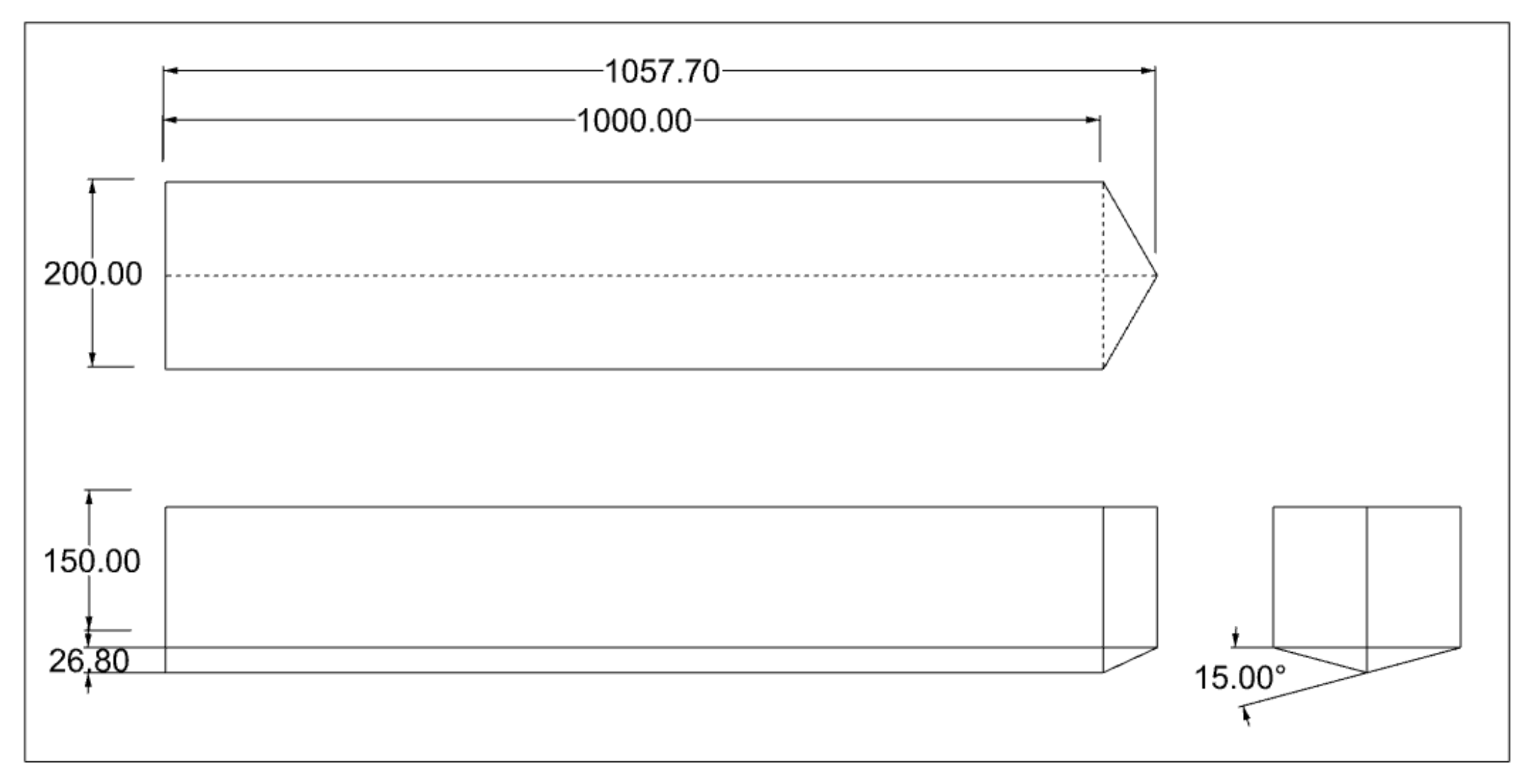
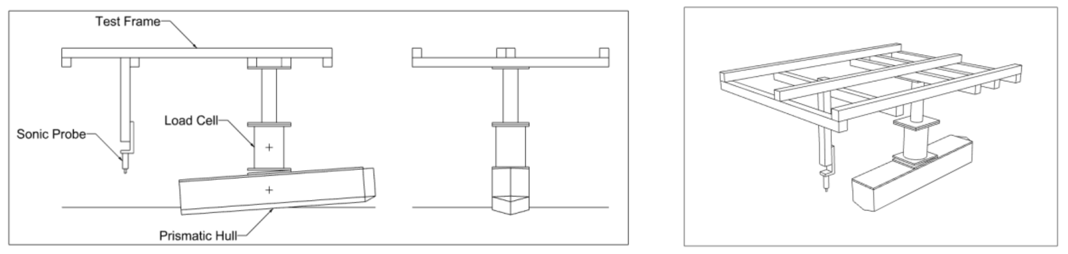
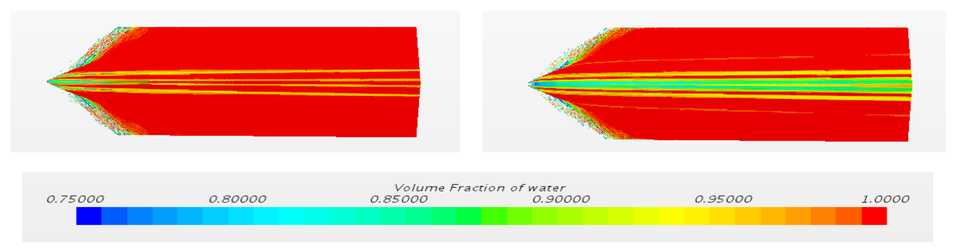
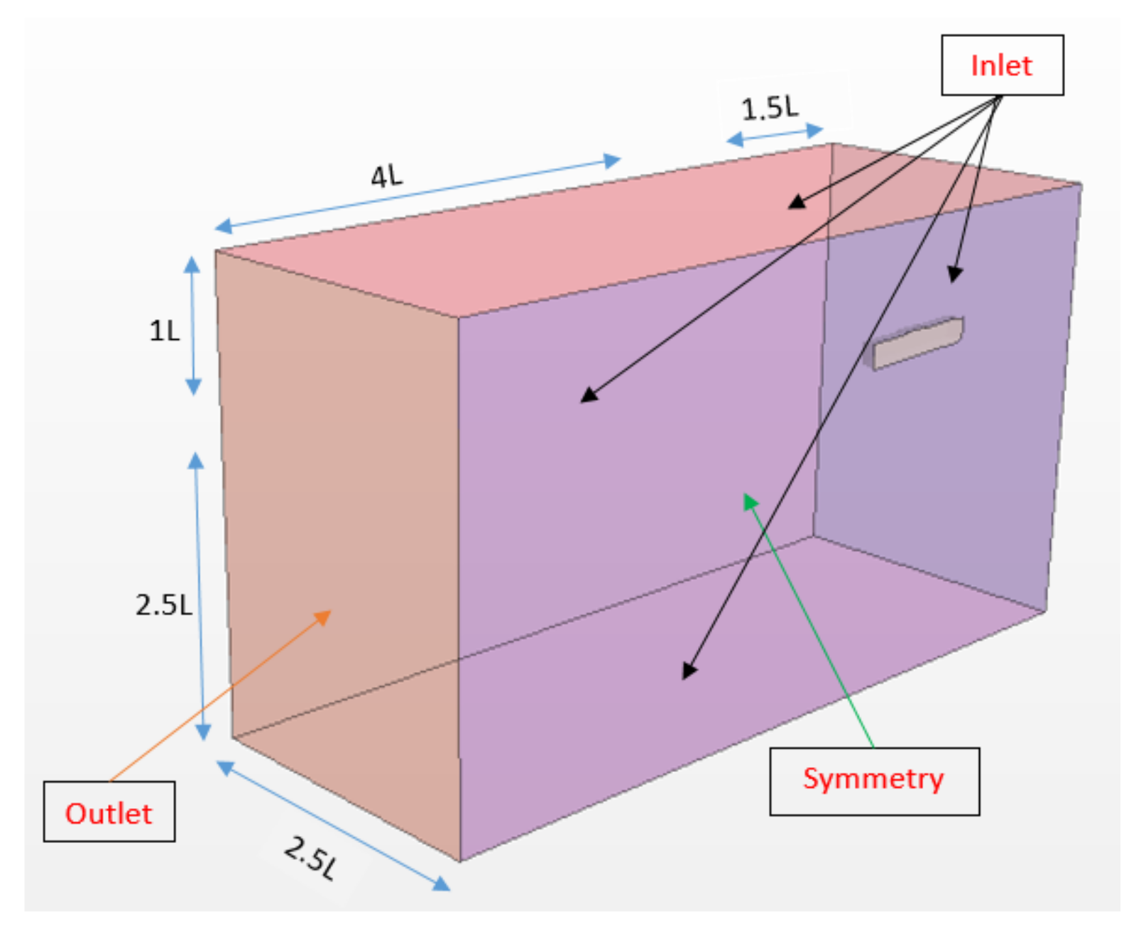
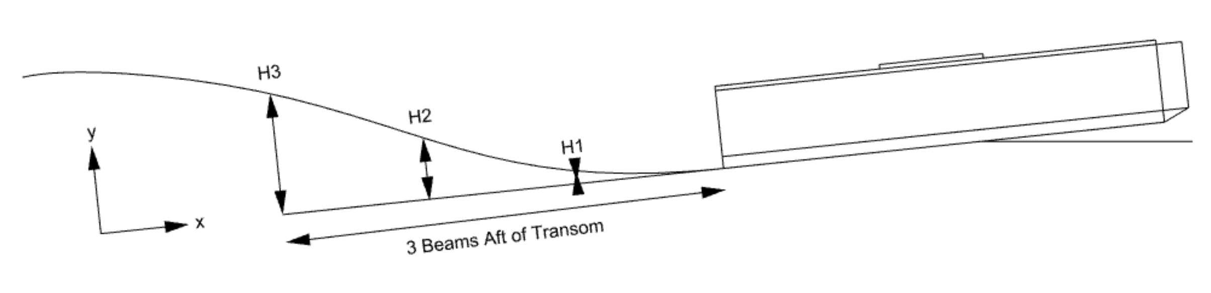
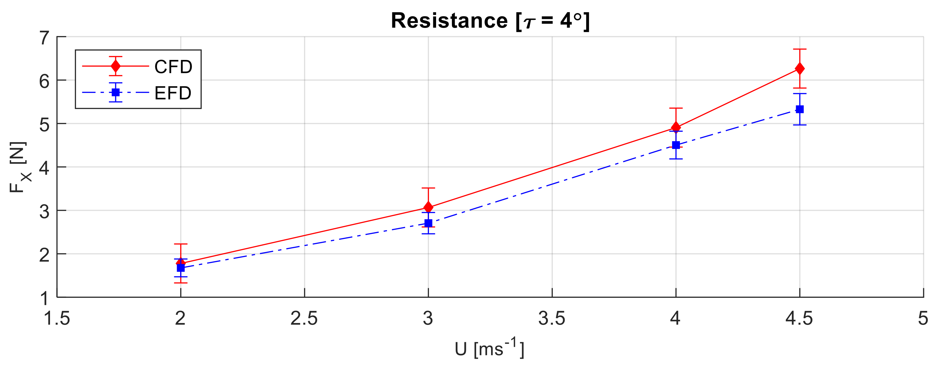
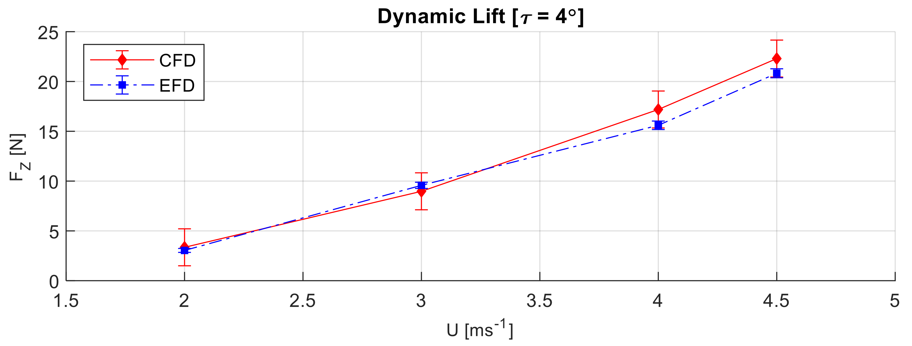
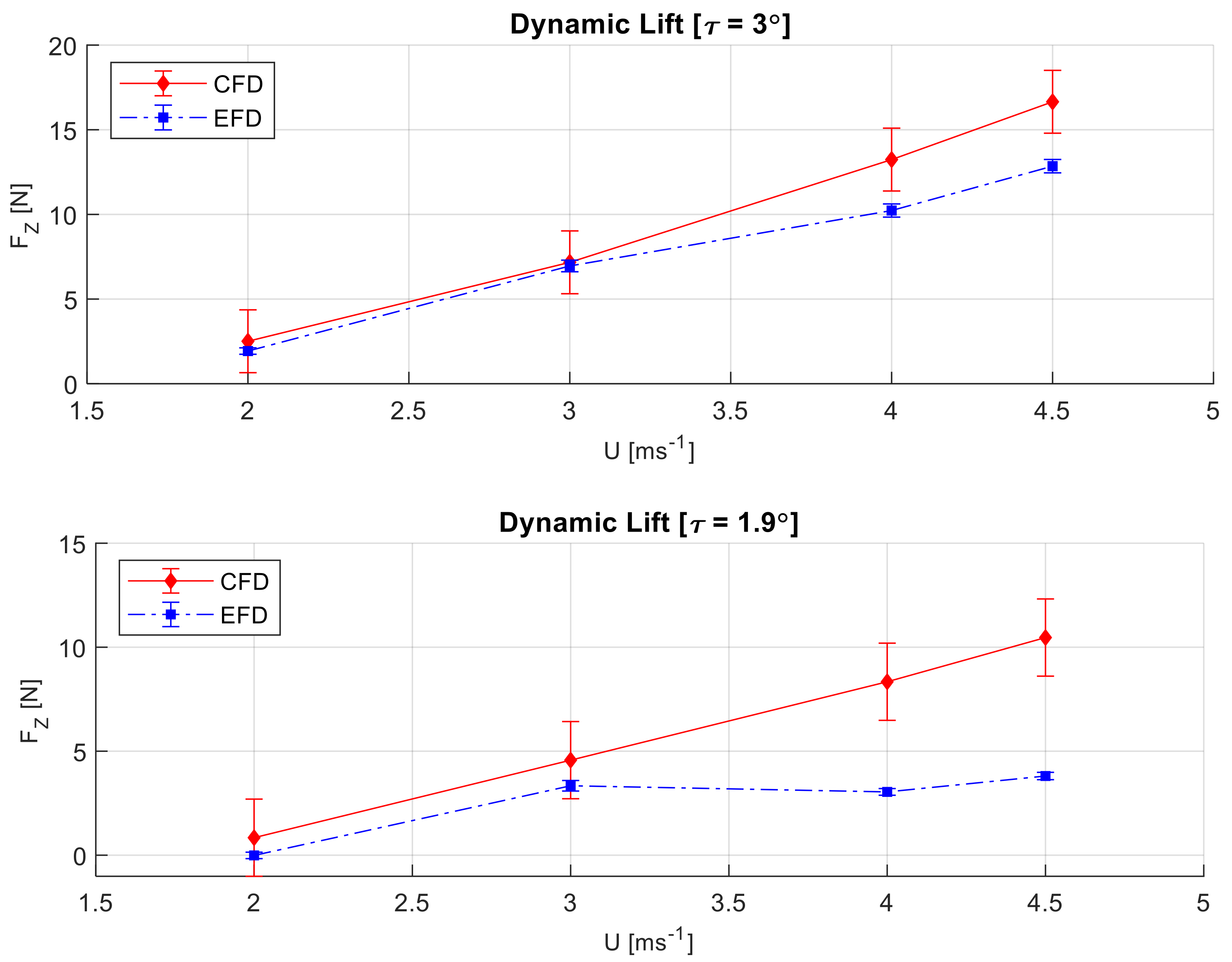
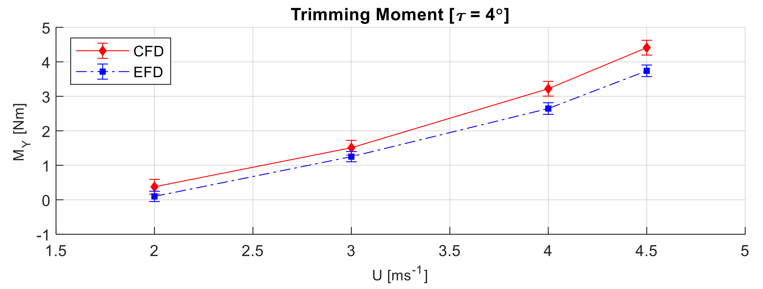
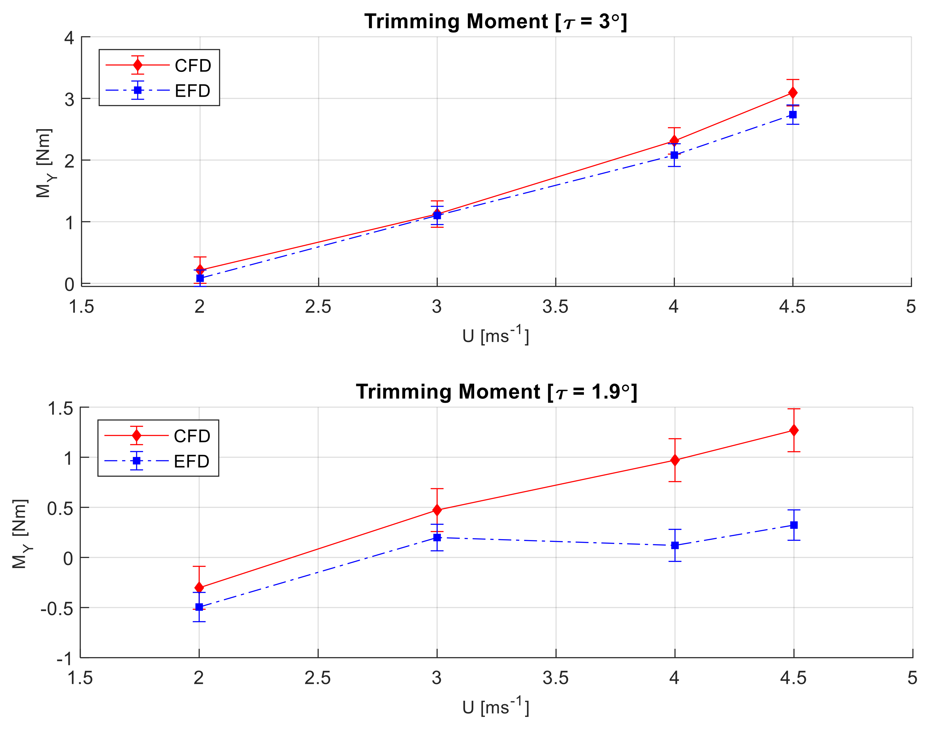
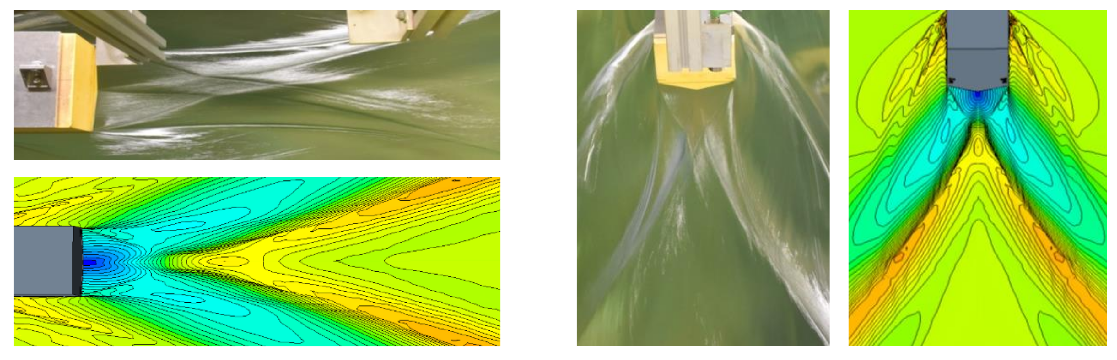
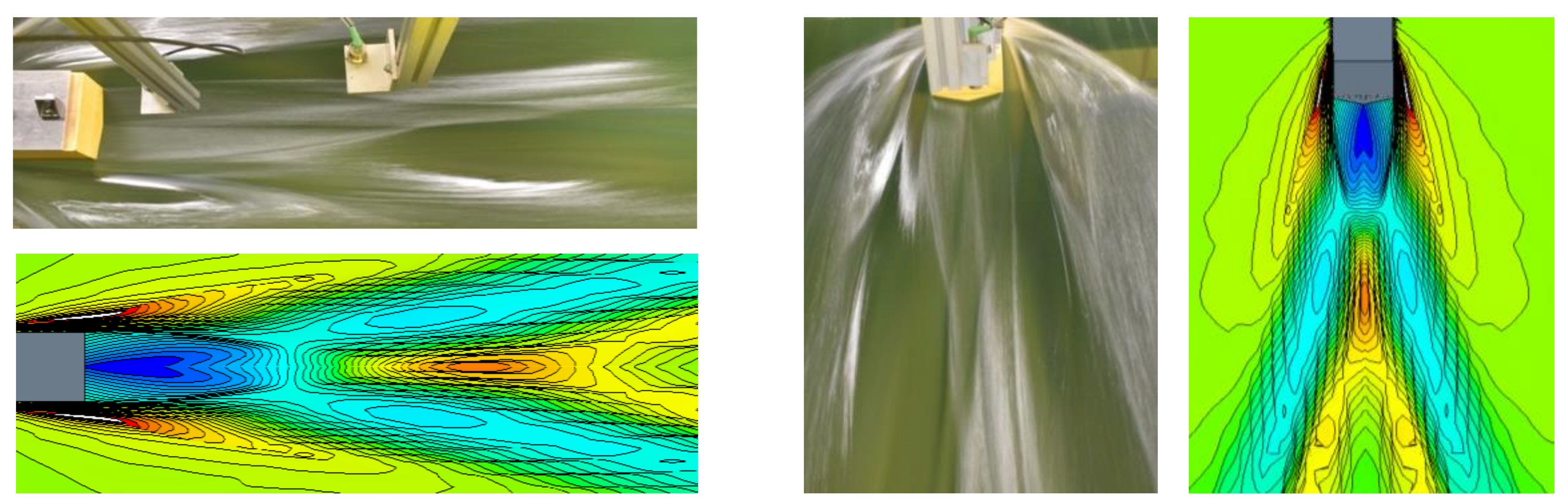
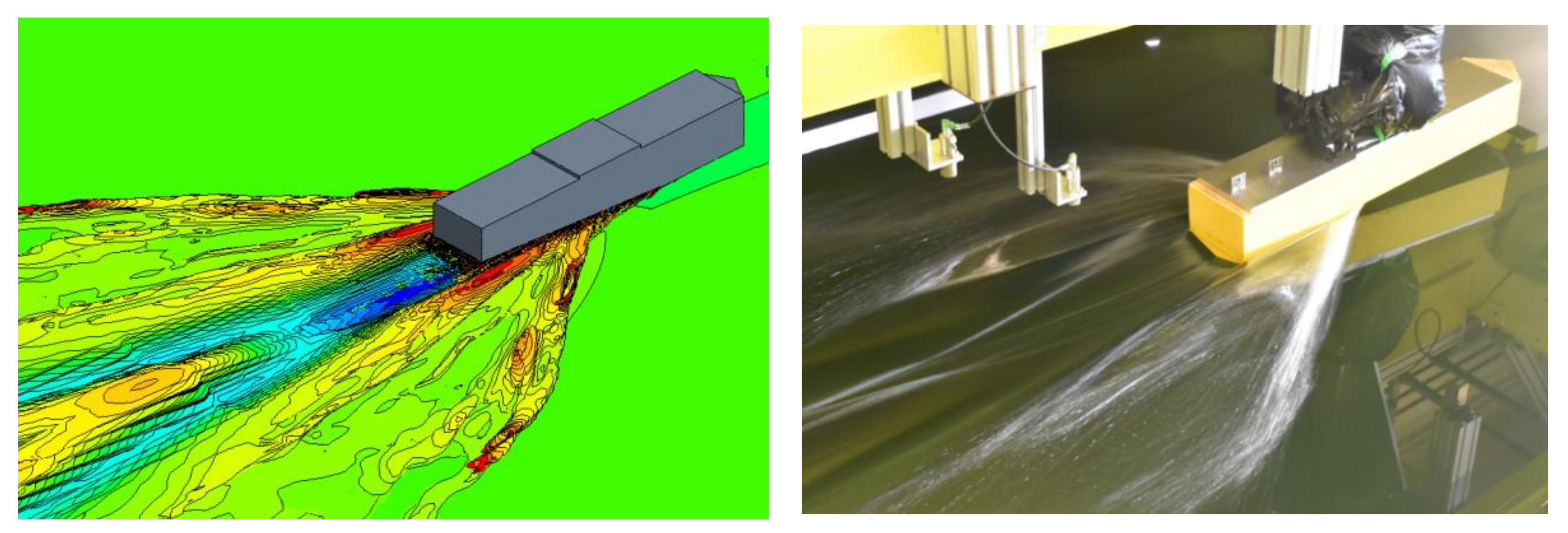
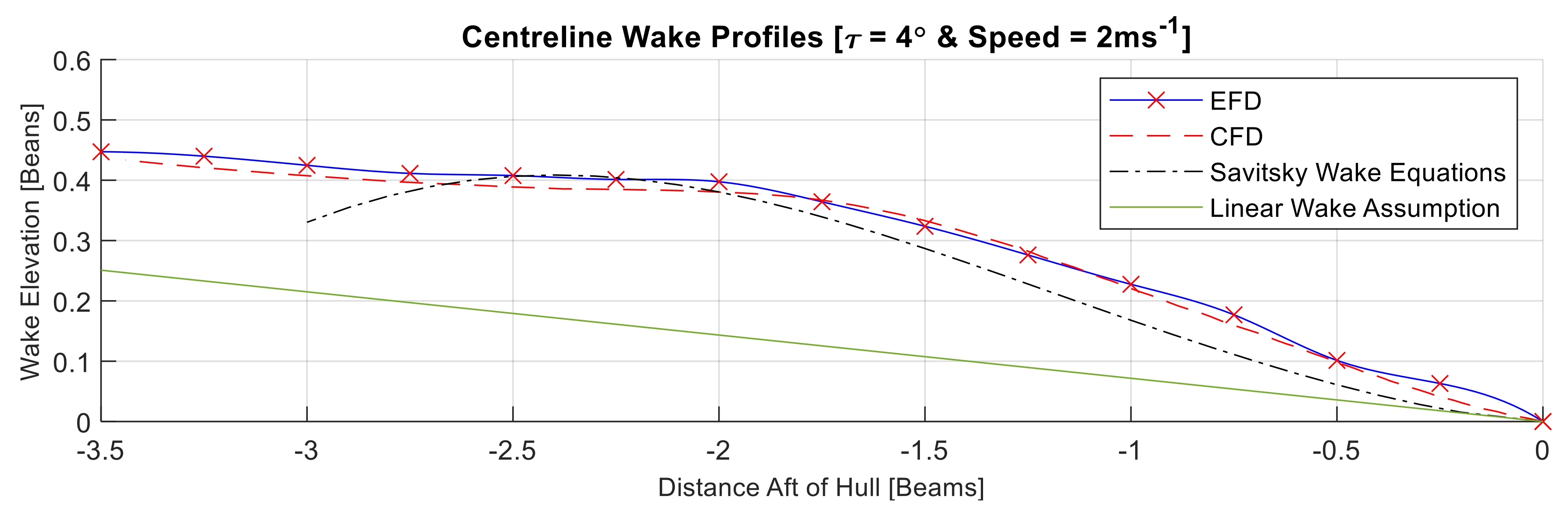
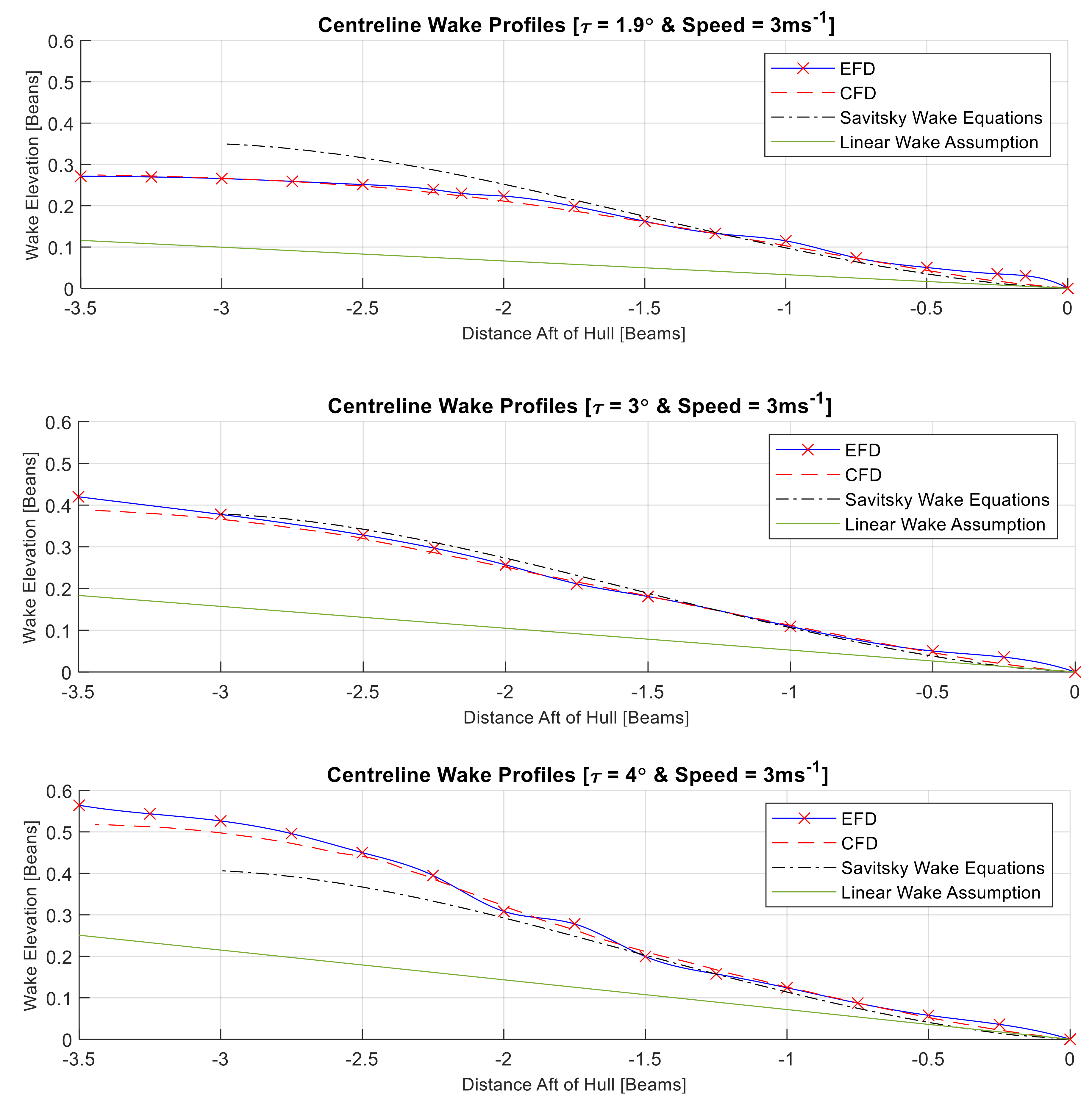
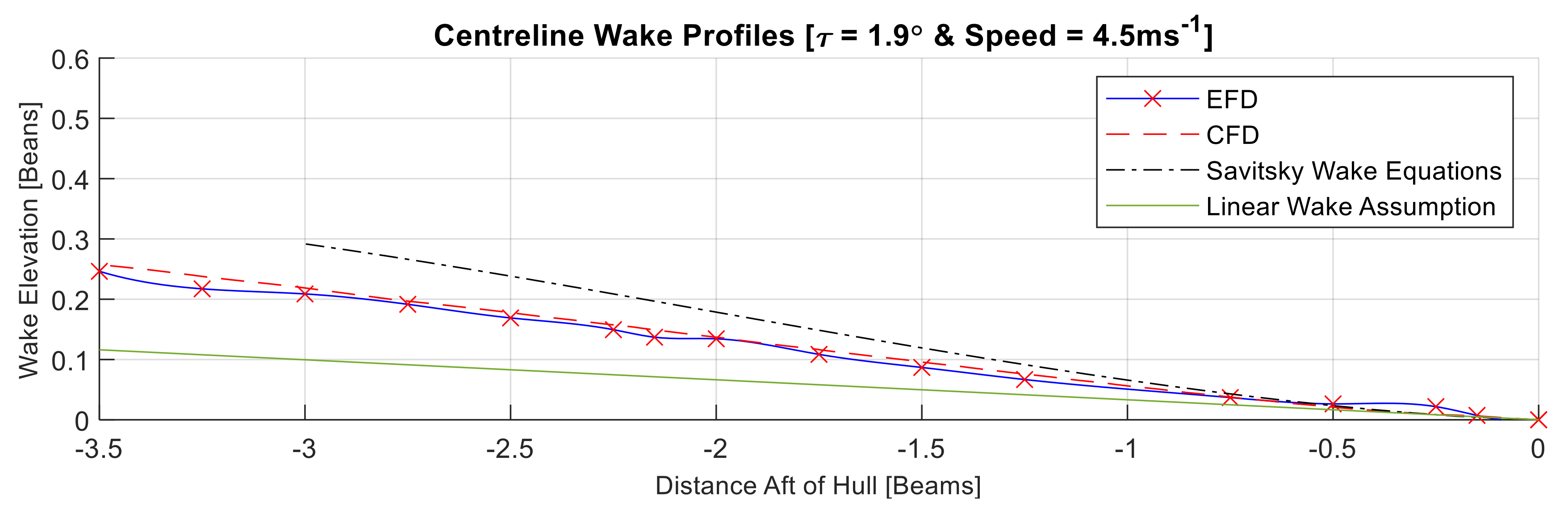
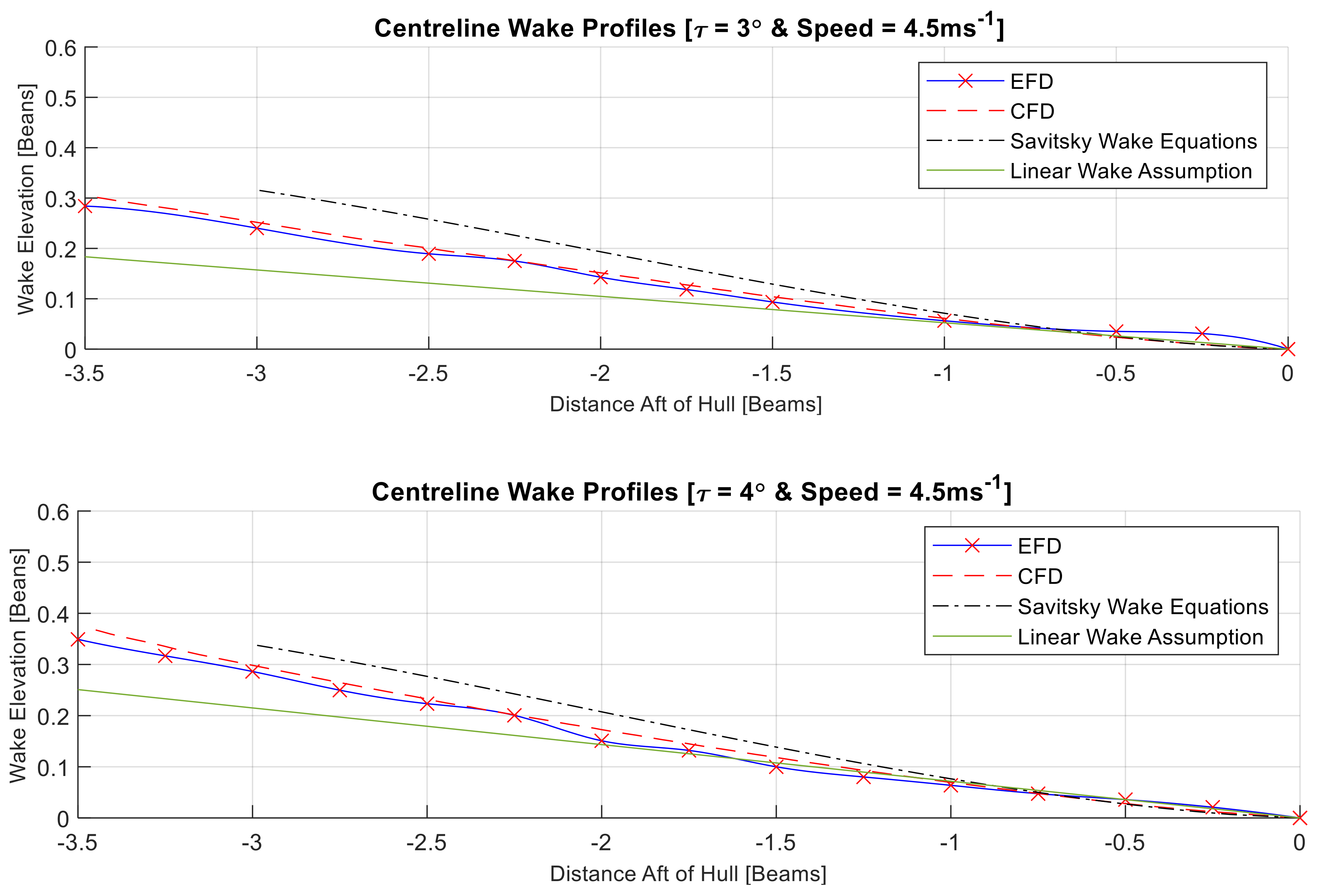
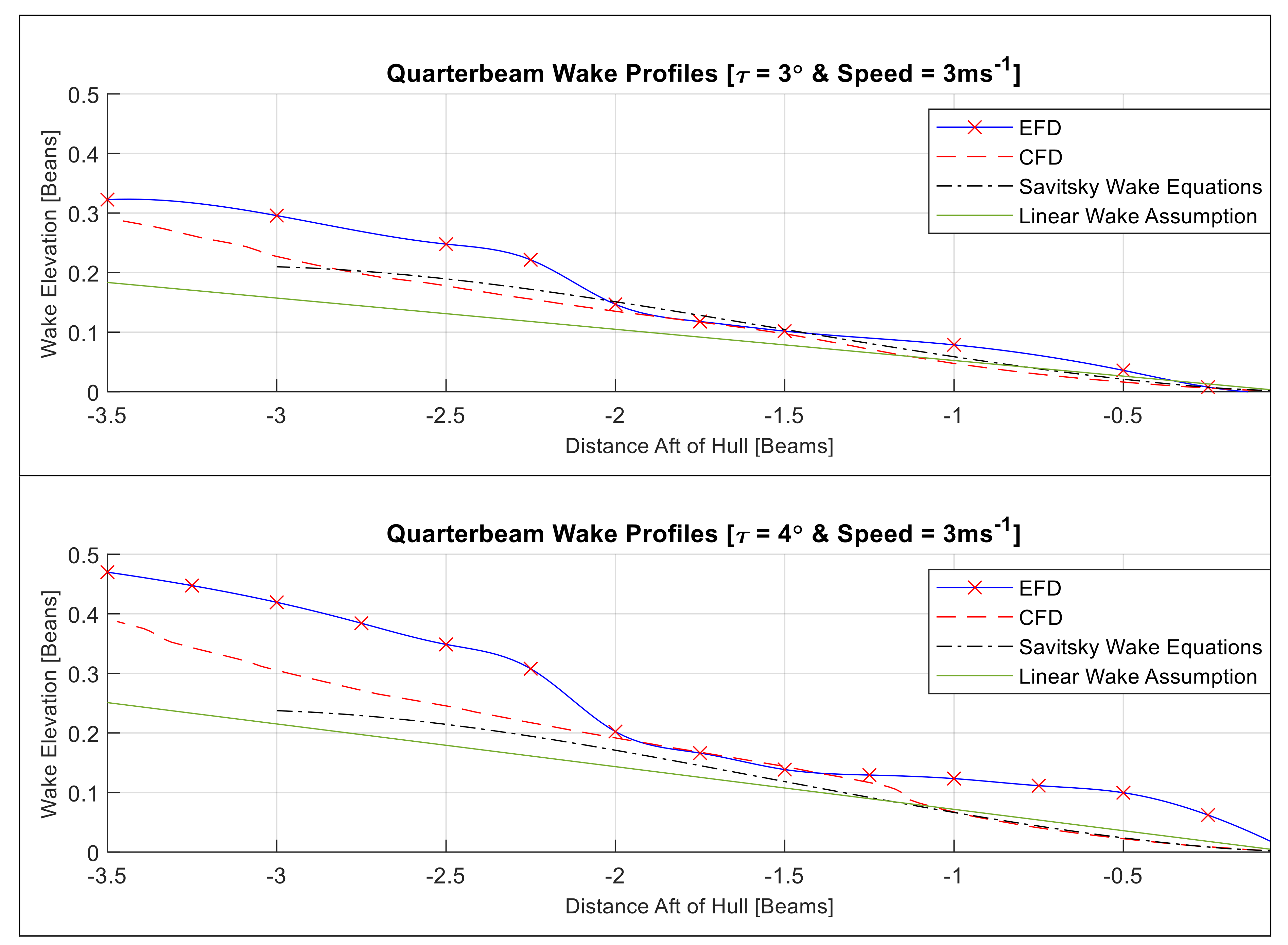
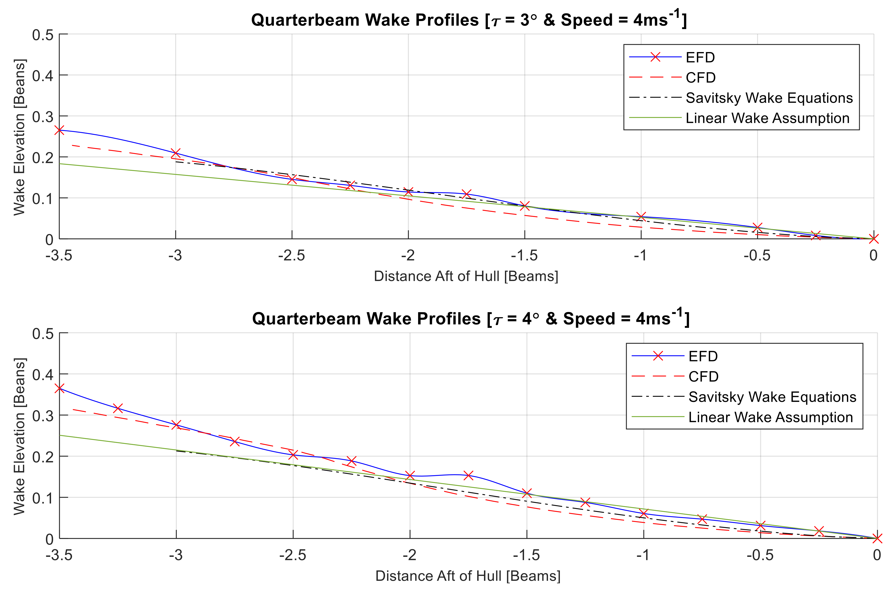
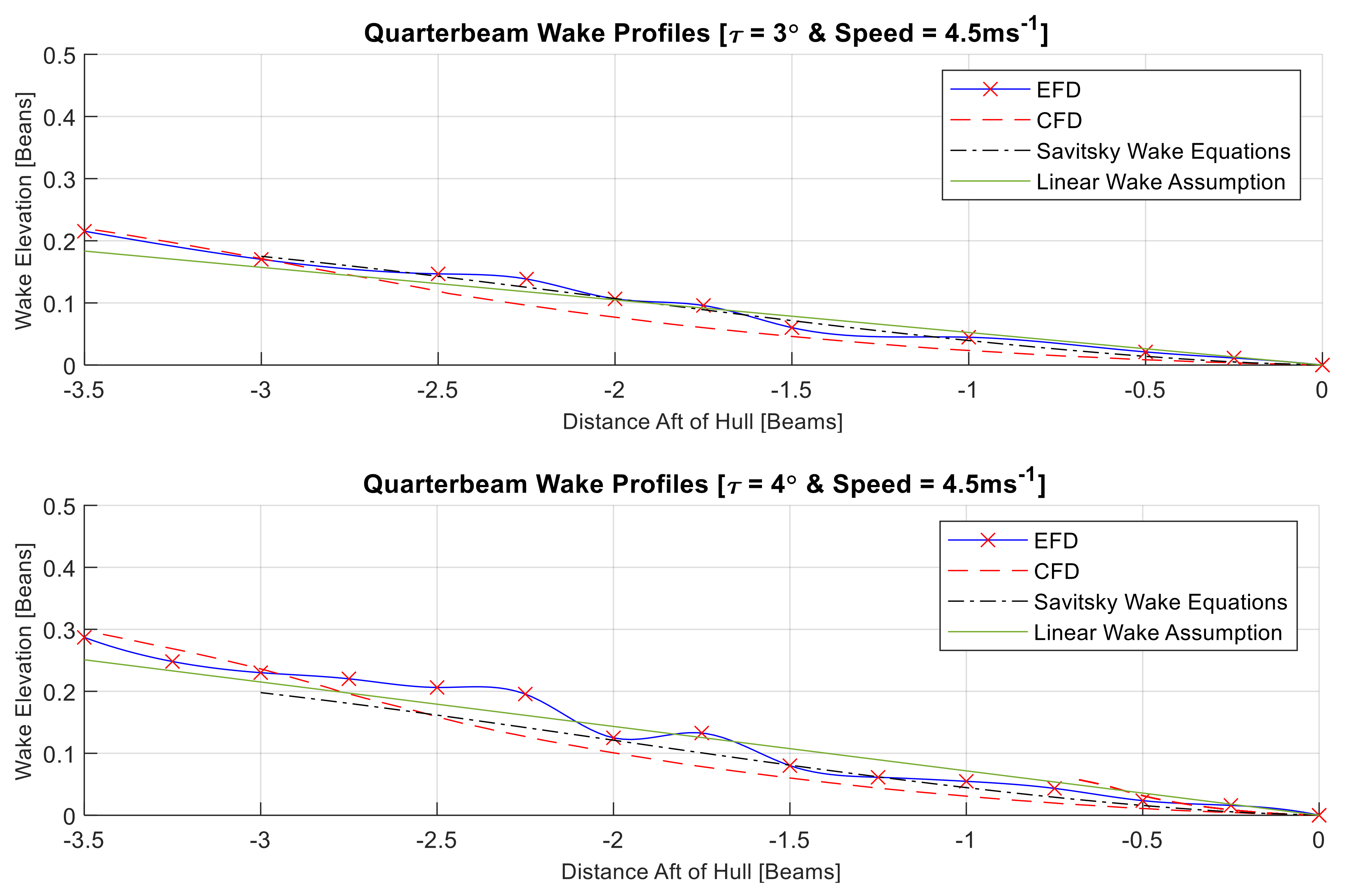