Influence of Growth and Recruitment Parameters in the Assessment and Management Variables of the Yellow Squat Lobster (Cervimunida johni)

Abstract

Fitting length data in age-structured stock assessment is a common method for evaluating hard-to-age animals, such as crustaceans. Growth specification and the uncertainty in the stock recruitment relationship are key issues in length-based assessment models. We conducted sensitivity analyses to evaluate the impact of growth and recruitment parameters on the stock assessment and management variables of the yellow squat lobster (Cervimunida johni) caught off the Chilean coast. Nine different scenarios of the length at first capture ($L_{a=1}$) and the coefficient of variation at age ($c{v}_a$) were tested for six combinations of values for the steepness parameter (h) and the recruitment variance (${\sigma }_R^2$). We also investigated the reliability of these estimates using an operating model. Our findings indicate that the parameter related to growth, $L_{a=1}$, has the greatest impact on the assessment and management variables of this fishery resource, with $c{v}_a$ having a lesser effect. Recruitment and fishing mortality estimates were the main variables affected. Parameters h and ${\sigma }_R^2$ did not profoundly impact the variables assessed. In addition, $L_{a=1}$ was the most biased estimated parameter. We discuss that the high influence of growth parameters is related to model structure, and thus implications for determination of the status of yellow squat lobster should be addressed in the future. We recommended developing simulation protocols for the selection of growth parameters when using an age-structured model with length observations, and we believe that our findings are relevant for all Chilean fisheries with a similar stock assessment framework.

1. Introduction

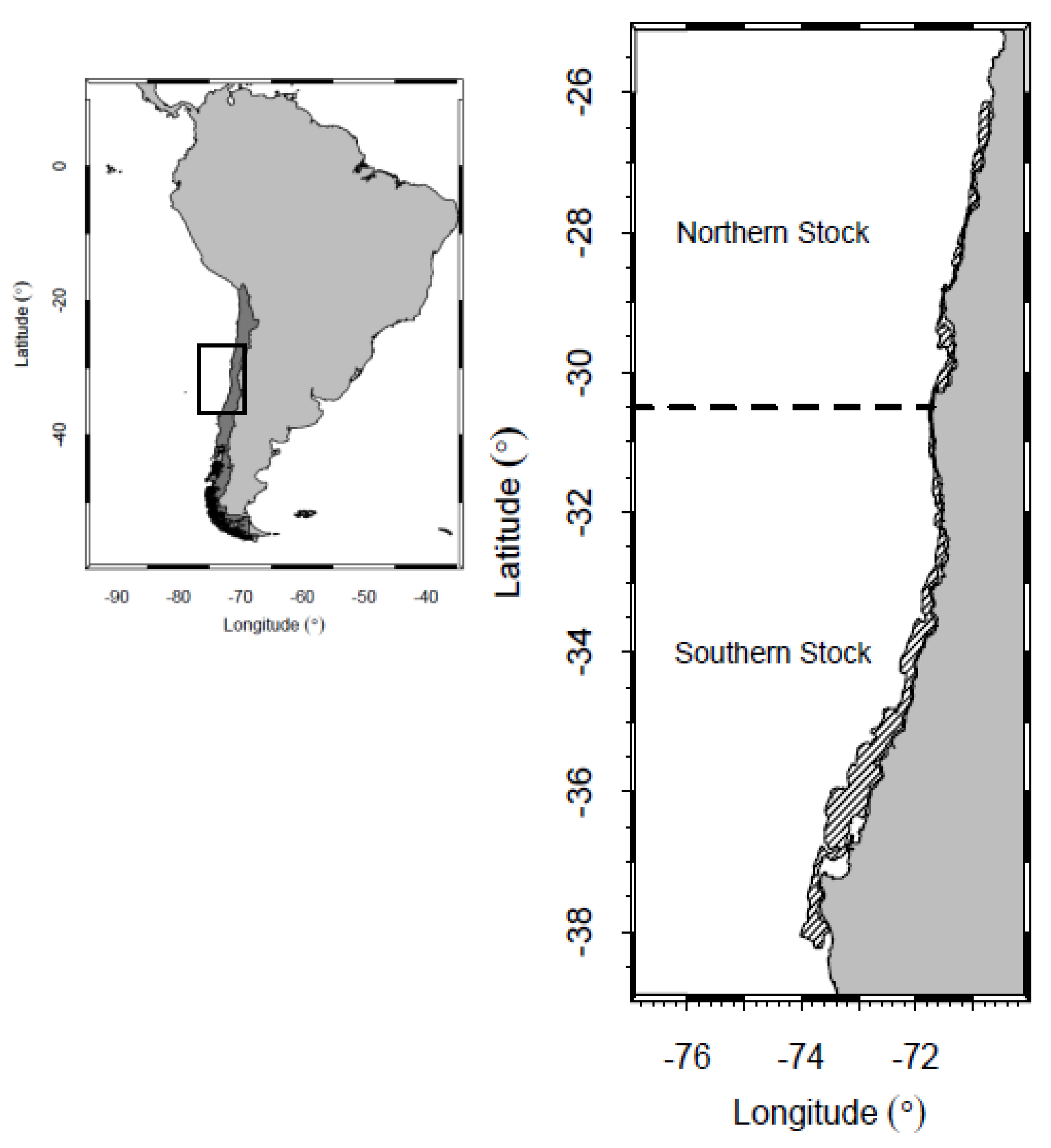
Yellow squat lobster (Cervimunida johni) is one of the most important crustaceans harvested in Chile in terms of landings and economical relevance. This species is a demersal crustacean inhabiting the Southeast Pacific coast between Taltal (29${}^{\circ }$19${}^{\prime }$ S) and Mocha Island (38${}^{\circ }$20${}^{\prime }$ S). Distribution is characterised by a narrow band on the continental shelf and upper part of the continental slope in depths of 100 to 500 m. The crustacean fishery in Chile started in the 1950s and features industrial and small-scale bottom trawlers, with a maximum landing of around 62,000 tons reached in 1976. Nowadays, landings of yellow squat lobster in Chile are around 5000 tons. Since 1996 this population has been separated into Northern Stock (26${}^{\circ }$03${}^{\prime }$ S–30${}^{\circ }$30${}^{\prime }$ S) and Southern Stock (30${}^{\circ }$30${}^{\prime }$ S–38${}^{\circ }$48${}^{\prime }$ S) (Figure 1) for management purposes. Management of yellow squat lobster in Chile is based on total allowed catch (TAC) and reproductive closures.

Since 1991, fisheries management in Chile has been regulated by the “general law of fishing and aquaculture” including a system for quota allocation based on individual transferable quotas (ITQs) from 2001 to 2012. The Chilean fishing law was amended in 2013 to incorporate, among other changes, the maximum sustainable yield (MSY) as target reference point for managing fishery resources. This mandate triggered the estimation of MSY-based reference points (MSY-RPs) in each fishery subject to catch limits in Chile [1].

In the case of the yellow squat lobster, MSY and depletion of spawning biomass are derived from an integrated age-structured stock assessment model, which combines data from different sources to estimate relevant population parameters. Direct assignation of age is difficult for crustaceans and debates still continue regarding the utility of age- or length-based stock assessment models [2]. However, even when age cannot be assigned directly, age-structured models are useful for estimating recruitment cohorts, making population dynamics more tractable [2].

For yellow squat lobster, the stock assessment is based on ages but fits observations of length structures; therefore, the conditional probability of the length-at-age (age-at-length key) is needed to convert observed lengths into ages. Age-at-length comes from individual growth parameters that are usually fixed within the stock assessment model. The assumption that growth parameters are known (for instance, updating) may add more uncertainty and complexity to the stock assessment of crustaceans, because small variations in growth parameters can have profound effects on the stock assessment and management variables and exploitation status [3]. Steepness (h) is a common measurement of stock resilience and is defined as the recruitment produced by a spawning biomass at 20% of unfished spawning biomass, relative to the recruitment produced by unfished spawning biomass [4]. Incorrect assumptions on the steepness parameter will directly affect the assessment variables and the specific level at which each stock can be harvested.

Despite the importance of both growth and recruitment processes for the assessment and management variables of yellow squat lobster in Chile, the impact of the assumed parameters has not yet been studied. Thus, the aim of this paper is to explore how different assumptions about the parameters used in the growth and the stock recruitment relationship (SRR) affect the assessment and management variables (e.g., spawning biomass) of the yellow squat lobster fishery off Chile. We develop a sensitivity analysis to investigate the impact of the variation of growth and recruitment parameters on the different assessment and management variables. Using the yellow squat lobster stock assessment model as an operating model, we implement an extensive simulation analysis to assess the reliability in the estimation of those parameters that caused the higher variation in management quantities (e.g., ratio between the spawning biomass in the last year and the unfished spawning biomass, $SB/S{B}_0)$. We conclude that the parameters that describe individual growth have the largest impact in the assessment and management variables of the yellow squat lobster stock and we believe that our findings are extensive to all Chilean fisheries using the same assessment framework.

2. Materials and Methods

To address the sensitivity and simulation analyses of the growth and recruitment parameters we used the most recent stock assessment model for yellow squat lobster [5]. Sensitivity analysis involved only realizations of the stock assessment model, but simulation analysis used an operating model with a simulation and estimation sections. A complete description of the operating model can be found in Section 2.2 and

Table 1. Parameter notation and description of the operating and estimation models. ★ indicate estimated parameter.

Symbol	Value	Description
Indices
s	2	Number of sex ($m:$ male; $f:$ female)
t	$1985,\dots ,$ t = 2015	Time (yrs)
a	$1,2,\dots ,$ a = 11	Number of age classes
l	$10,11,\dots ,$ l $=52$	Number of length bins
Observed data
$P_{l,t,s}$		Proportion of catch-at-length
$P_{l,t,s}^{\Omega }$		Proportion of abundance-at-length from survey
$cpu{e}_t$		Annual catch per unit of effort
$Y_t$		Annual landing
$I_t$		Annual index from research survey
$p_t^m$		Annual proportion of males in the total landing
Parameters
$L_{\infty ,s}$	$m=52.8$; $f=45.6$	Asymptotic length (mm)
$k_s$	$m=0.151$; $f=0.174$	von Bertalanffy growth coefficient
$R_0$	★	Unfished recruitment
${\sigma }_R^2$	0.6	Standard error of log-recruitment deviations
${\sigma }_{{\eta }_s}^2$	0.6	Standard error of initial log-abundance
$L_{a=1,s}$	$m=20.4$; $f=13.7$	Mean length of the first age class (mm)
$c{v}_{a,s}$	$m=0.083$; $f=0.037$	Coefficient of variation of the length-at-age
q	★	Catchability coefficient for commercial fishing
$q^{\Omega }$	★	Catchability coefficient for research survey
$a_s^{50},a_s^{95}$	★	Selectivity function parameters for commercial fishing
${\Omega }_s^{50},{\Omega }_s^{95}$	★	Selectivity function parameters for survey
$F_{t,s}$	★	Annual fishing mortality rate
M	0.12	Instantaneous natural mortality rate
h	1	Steepness stock-recruitment relationships
${\eta }_{a,s}$	★
${\tilde{p}}_t^m$	★
Derived variables
$s{b}_0$		Unfished equilibrium spawning biomass per recruit
${\mathrm{SB}}_0$		Unfished spawning biomass
$l_{a,s}$		Length-at-age
$m_{a,s}$		Proportion maturity-at-age
${\omega }_{a,s}$		Body mass-at-age
$N_{a,t,s}$		Abundance of fish
${\mathrm{SB}}_t$		Spawning biomass
${\mathrm{MN}}_{a,t,s}$		Mid-year abundance
${\overline{R}}_{t,s}$		Annual Recruitment by sex
${\tilde{p}}_t^s$		Sex ration of total recruitment ${\overline{R}}_t$
${\mathrm{VB}}_t$		Vulnerable biomass to commercial fishing
${\mathrm{VB}}_t^{\Omega }$		Vulnerable biomass to research survey
$\alpha ,\beta$		Beverton Holt stock recruitment parameters
$p(l\mid a)$		Sex-based age−length key
${\sigma }_{a,s}$		Standard deviation of length-at-age
$C_{a,t,s}$		Catch-at-age
$Y_t$		Annual landing
${\varphi }_{a,s}$		Selectivity -at, -age and -sex

,

Table 2. Definition of equations for operating and estimation models.

Process / Equation	Description	Form
Growth
Equation (1)	Length-at-age	$l_{a,s}=L_{\infty ,s}(1-e^{-k_s})+e^{-k_s}{l}_{a-1}$
Equation (2)	Variation of length-at-age	$c{v}_{a,s}=\frac{{\sigma }_{a,s}}{l_{a,s}}$
Equation (3)	Probability of length-at-age	$p(l_s\mid a)=\frac{1}{\sqrt{2\pi {\sigma }_{a,s}}}{e}^{-}\frac{{(l_s-l_{a,s})}^2}{2{\sigma }_{a,s}^2}$
Stock recruitment relationship
Equation (4)	Beverton and Holt (BH) function	${\overline{R}}_t=\frac{\alpha {\mathrm{SB}}_{t-1}}{\beta +{\mathrm{SB}}_{t-1}}{e}^{({\epsilon }_t-\frac{{\sigma }_R^2}{2})},{\epsilon }_t\sim \mathrm{N}(0,{\sigma }_R^2)$
Equation (5)	Parameter of BH function	$\alpha =\frac{4h{R}_0}{5h-1}$
Equation (6)	Parameter of BH function	$\beta =\frac{(1-h){\mathrm{SB}}_0}{5h-1}$
Equation (7)	Average recruitment	${\overline{R}}_{t,s}={\tilde{p}}_t^s{\overline{R}}_t$
Initial Condition, Fished equilibrium at $t=1$
Equation (8)	Unfished spawning biomass	${\mathrm{sb}}_0={\sum }_{a=1}^{A-1}{m}_{a,s}{\omega }_{a,s}{e}^{-M(a-1)}+\frac{m_{a,s}{\omega }_{a,s}{e}^{-M(A-1)}}{1-e^{-M}},s=f$
Equation (9)	Initial abundance-at-age	$N_{a,s}=\left\{\begin{array}{cc}{\tilde{p}}_t^s{R}_0,\hfill & a=1\hfill \\ N_{a-1,s}{e}^{-M},\hfill & 1<a\le A\hfill \\ \frac{N_{a-1,s}{e}^{-M}}{1-e^{-M}},\hfill & a=A,\hfill \end{array}\right.$
Equation (10)	Initial abundance-at-age with process error	$N_{a,s}=N_{a,s}{e}^{({\eta }_{a,s}-\frac{{\sigma }_{\eta }^2}{2})},{\eta }_{a,s}\sim \mathrm{N}(0,{\sigma }_{{\eta }_s}^2)$
State Dynamics at $t>1$
Equation (11)	Abundance-at-age	$N_{a,t,s}=\left\{\begin{array}{c}{\overline{R}}_{t,s},a=1\hfill \\ N_{a-1,t-1,s}{e}^{-M-s_{a,s}{F}_{t,s}},1<a\le A\hfill \\ N_{a-1,t-1,s}{e}^{-M-s_{a,s}{F}_{t,s}}+N_{a,t-1,s}{e}^{-M-s_{a,s}{F}_{t,s}}\hfill \end{array}\right.$
Equation (12)	Spawning biomass	${\mathrm{SB}}_{t,s}={\sum }_{a=1}^A{N}_{a,t,s}{m}_{a,s}{\omega }_{a,s},s=f$
Equation (13)	Catches	$C_{a,t,s}=\frac{s_{a,s}{F}_{t,s}}{M+s_{a,s}{F}_{t,s}}{N}_{a,t,s}{e}^{(1-e^{-M-s_{a,s}{F}_{t,s}})}$
Equation (14)	Yield	$Y_t={\sum }_{s=1}^2{\sum }_{a=1}^A{C}_{a,t,s}{\omega }_a$
Fishery and Survey
Equation (15)	Fishery selectivity-at-age	$s_{a,s}=1/(1+e^{-\ln \left(19\right)\frac{a-a_s^{50}}{a_s^{95}-a_s^{50}}}$)
Equation (16)	Survey selectivity-at-age	$s_{a,s}^{\Omega }=1/(1+e^{-\ln \left(19\right)\frac{a-{\Omega }_s^{50}}{{\Omega }_s^{95}-{\Omega }_s^{50}}}$)
Equation (17)	Vulnerable mean abundance	${\mathrm{MN}}_{a,t,s}=N_{a,t,s}\frac{1-e^{-M-s_{a,s}{F}_{t,s}}}{M+s_{a,s}{F}_{t,s}}$
Equation (18)	Fishery Vulnerable Biomass	${\mathrm{VB}}_t={\sum }_{s=1}^2{\sum }_{l=1}^A{s}_{a,s}{\mathrm{MN}}_{a,t,s}p(l_s\mid a)w_{l,s}$
Equation (19)	Survey Vulnerable Biomass	${\mathrm{VB}}_t^{\Omega }={\sum }_{s=1}^2{\sum }_{a=1}^A{s}_{a,s}^{\Omega }{\mathrm{MN}}_{a,t,s}p(l_s\mid a)w_{l,s}$
Equation (20)	Catch per unit effort	${\mathrm{cpue}}_t=q{\mathrm{VB}}_t$
Equation (21)	Survey Biomass Index	${\mathrm{I}}_t=q^{\Omega }{\mathrm{VB}}_t^{\Omega }$
Equation (22)	Catchability	$q=e^{(\frac{1}{n_f}{\sum }_{t=1}^{n_f}\ln \left({\mathrm{cpue}}_t\right)-\ln \left({\mathrm{VB}}_t\right))}$

and

Table 3. Estimation model. Likelihood, penalties and the set of estimated parameters $\Theta$.

Process / Equation	Description	Form
Fishery
Equation (23)	Proportion catch-at-length	$P_{l,t,s}=\frac{C_{a,t,s}p(l_s\mid a)}{{\sum }_{l=1}^L{C}_{a,t,s}p(l_s\mid a)}$
Equation (24)	CPUE index	$L_1=n_{ϵ}\ln \left({\sigma }_{ϵ}\right)+\frac{1}{2{\sigma }_{ϵ}^2}{\sum }_{t=1}^{n_{ϵ}}\ln {\left(\frac{{\mathrm{cpue}}_t}{{\mathrm{cpue}}_t^o}\right)}^2$
Equation (25)	Fishery age-data	$L_2=-{\sum }_{t=1}^{n_l}{\sum }_{s=1}^2{\sum }_{a=1}^A{n}_m{P}_{l,t,s}^o\ln \left(P_{l,t,s}\right)$
Equation (26)	Total landing	$L_3=n_y\ln \left({\sigma }_y\right)+\frac{1}{2{\sigma }_y^2}{\sum }_{t=1}^{n_y}\ln {\left(\frac{Y_t}{Y_t^o}\right)}^2$
Survey
Equation (27)	Proportion survey-at-age	$P_{l,t,s}^{\Omega }=\frac{s_{a,s}^{\Omega }{\mathrm{MN}}_{a,t,s}p(l\mid a)}{{\sum }_{l=1}^L{s}_{a,s}^{\Omega }{\mathrm{MN}}_{a,t,s}p(l\mid a)}$
Equation (28)	Survey index	$L_4=n_{\iota }\ln \left({\sigma }_{\iota }\right)+\frac{1}{2{\sigma }_{\iota }^2}{\sum }_{t=1}^{n_{\iota }}\ln {\left(\frac{{\mathrm{I}}_t}{{\mathrm{I}}_t^o}\right)}^2$
Equation (29)	Survey age-data	$L_5=-{\sum }_{t=1}^{n_s}{\sum }_{s=1}^2{\sum }_{a=1}^{A}n{P}_{l,t,s}^{o\Omega }\ln \left(P_{l,t,s}^{\Omega }\right)$
Sex ratio
Equation (30)	Male proportion	${\tilde{p}}_t^m=\frac{{\sum }_{a=1}^A{s}_{a,s=m}{\mathrm{MN}}_{a,t,s=m}}{{\sum }_{s=1}^2{\sum }_{a=1}^A{s}_{a,s}{\mathrm{MN}}_{a,t,s}}$
Equation (31)	Sex ratio	$L_6=\frac{{\sum }_{t=1}^{T_p}{(p_t^m-{\tilde{p}}_t^m)}^2}{2{\tilde{p}}_t^m(1-{\tilde{p}}_t^m)/n}$
Penalties
Equation (32)	Annual recruitment	$P_1=\frac{1}{{\sigma }_R^2}{\sum }_{t=1}^T{\epsilon }_t^2$
Equation (33)	Initial abundance-at-age	$P_2=\frac{1}{{\sigma }^{\eta }}{\sum }_{a=1}^A{\eta }_a^2$
Total Likelihood
Equation (34)	Total Likelihood	$L_T={\sum }_{k=1}^6{L}_k+{\sum }_{j=1}^2{P}_j$
Estimated parameters
Equation (35)		$\Theta =\left\{R_0,{\epsilon }_t,{\eta }_{a,s},l_{1,s},c{v}_{a,s},F_{t,s},a_s^{50},a_s^{95},{\Omega }_s^{50},{\Omega }_s^{95},q^{\Omega }\right\}$

.

2.1. Testing the Growth and Recruitment Parameters

A base case scenario is required as a benchmark to study the impact on the status and management variables of the changes of the length at first capture $L_{a=1}$, variation of the length at a given age $c{v}_a$, recruitment variance (${\sigma }_R^2$) and steepness (h) of the stock recruitment relationship (SRR). The first two parameters are involved in the growth process, while ${\sigma }_R^2$ and h controls the variability of the SRR and the dependence of the recruitment on spawning biomass, respectively.

The base case scenario assumes fixed parameters for recruitment variance, ${\sigma }_R^2=0.6$ and steepness, $h=1$. Values of these parameters were chosen based on results obtained in previous stock assessment reports [5] for yellow squat lobster in which recruitment variability is moderate (not exceed $cv=0.6$) and recruitments show low dependency of the spawning biomass size. Note that $h=1$ means that reductions in spawning biomass will not affect recruitments. Likewise, growth parameters ($L_{a=1}$, $c{v}_a$) in the base case scenario were taken from reports [5] and they were fixed to the following values: $L_{a=1}=13.7$ (cm) and $c{v}_a=0.037$ for females, and $L_{a=1}=20.4$ (cm) and $c{v}_a=0.083$ for males.

Like many crustacean species, yellow squat lobster shows an important sexual dimorphism, which leads to differences in the growth traits [6], reflecting gender differences on the length at first capture. In the case of length variability at age, empirical studies of growth for yellow squat lobster based on age do not exist, therefore model-based studies are simplified by using a constant $c{v}_a$ which involve a positive causal relationship between the average length at age and its variance [5,7]

Nine scenarios were evaluated containing a pair combination of different values of $L_{a=1}$ and $c{v}_a$ (

Table 4. Scenarios of the mean length at first capture ($L_{a=1}$) and the variation of the length-at-age ($c{v}_a$). (Base = base case scenario).

Scenarios	${\mathit{L}}_{\mathit{a}=1}$	${\mathit{cv}}_{\mathit{a}}$
1	−10%	−10%
2	Base	−10%
3	+10%	−10%
4	−10%	Base
5	Base	Base
6	+10%	Base
7	−10%	+10%
8	Base	+10%
9	+10%	+10%

). Previous analyses on the stock assessment model [5] showed that changes in the selectivity function produces variability on $L_{a=1}$ no greater than ∼2 cm. Therefore, to match this variation we consider scenarios for $L_{a=1}$ of around ±10% (Table 4). Similarly, variability on $c{v}_a$ was also set to ±10% across scenarios. Parameter $c{v}_a$ controls the variability of the length-at-age and it needs to be constrains to a narrow range on the simulation in order to control the degree of overlapping among cohorts to biological meaning scenarios. Once values of $L_{a=1}$ and $c{v}_a$ were chosen for each simulation scenario, they were fixed at each realization of the stock assessment model.

In order to analyse the impact of the SRR parameters, we implemented different combinations of ${\sigma }_R^2$ and h. Values for h were chosen as the values used on the stock assessment, lower bound $h=0.75$ and higher bound $h=1$ [5]. In addition the value of $h=0.75$ defines the most common shape of the SRR [8]. Six combinations of steepness values of 0.75 and 1, and ${\sigma }_R^2$ of 1, 0.6 and 0.2 were assessed. Each scenario of $L_{a=1}$ and $c{v}_a$ in Table 4, was a realization for each combination of ${\sigma }_R^2$ and h (

Table 5. Combinations of the steepness (h) values and recruitment variance (${\sigma }_R^2$) for each of nine scenarios of $L_{a=1}$ and $c{v}_a$.

	h	${\mathit{\sigma }}_{\mathit{R}}^2$	No scenarios of ${\mathit{L}}_{\mathit{a}=1}$ and ${\mathit{cv}}_{\mathit{a}}$
Combination 1	1.0	0.2	9
Combination 2	1.0	0.6	9
Combination 3	1.0	1.0	9
Combination 4	0.75	0.2	9
Combination 5	0.75	0.6	9
Combination 6	0.75	1.0	9

). A total of 54 realizations were computed to explore the effect on the stock assessment and management variables of the parameters assumed in both the growth and recruitment processes. Because the stock assessment accounts for differences in growth between males and females the variation of $L_{a=1}$ and $c{v}_a$ (Table 4) were applied to males and females.

To study the impact of the changes of these parameters on the assessment and the resulting management estimates we used the following variables—Total biomass in the last year ($TB$); spawning biomass in the last year ($SB$); average recruitment (R); yield at MSY ($Y_{MSY}$); unfished spawning biomass ($S{B}_0$); ratio between last year yield (Y) and yield at MSY ($Y/Y_{MSY}$); ratio between the fishing mortality in the last year (F) and fishing mortality at MSY ($F/F_{MSY}$); ratio between the $SB$ in the last year and the unfished spawning biomass ($SB/S{B}_0$); fishing mortality of the last year (F), and the target fishing mortality ($F_{MSY}$). All these measures were standardized to the base case scenario, which means each assessment and management variable generated in each scenario of Table 4 and Table 5 was divided by the value of the same variable in the base case scenario.

2.2. Reliability of the Parameters Estimation

A simulation analysis was developed for $L_{a=1}$, $c{v}_a$ and h. The operating model assumes a sex-based age-structured population dynamics, with an annual recruitment pulse modelled using the Beverton-Holt SRR. Since there are not reported catches before 1985, the initial age-structure abundance vector is assumed under a fished equilibrium state. The growth process uses an age-at-length key that assumes known growth parameters (k and $L_{\infty }$). Parameters $L_{a=1}$, $c{v}_a$ and h are estimated simultaneously with others relevant parameters such as unfished recruitment, initial abundance deviations, annual recruitment errors and fishing mortality. A detailed description of the operating model appears in Table 1, Table 2 and Table 3. See Table 1 for notation of parameters and derived variables.

Parameters of the stock assessment model were estimated using maximum likelihood estimation (MLE). Seven sources of data are used to maximise the total log-likelihood function defined in Table 3: (i) official landings, (ii) standardised catch per unit effort (CPUE), (iii) fisheries-independent biomass index (annual swept area surveys), (iv) length compositions from the commercial fleets and surveys, (v) annual female proportion in the landings, (vi) medium weight at length for each sex and (vii) female maturity ogive. Selectivity is assumed constant over time for the fishery and survey. The MSY is independent of the SRR and obtained from proxy values [9]. The model was implemented using the software AD Model Builder for non-linear statistical modelling [10].

The simulation model was conditioned to the data and errors of the base case scenario [5]. Process error of the annual recruitment was simulated assuming a value ${\sigma }_R^2=0.6$ in all simulations. Thus, two simulations were developed by varying the value of $L_{a=1}$ and h (

Table 6. Simulation trials to explore the predictability of the growth parameters $L_{a=1}$ and $c{v}_a$ and productivity (h) with the assumption of a ${\sigma }_R^2=0.6$. (Base = base case scenario).

	Simulator				Estimator
	${\mathit{L}}_{\mathit{a}=\mathbf{1}}$	${\mathit{cv}}_{\mathit{a}}$	$\mathit{h}$		${\mathit{L}}_{\mathit{a}=\mathbf{1}}$	${\mathit{cv}}_{\mathit{a}}$	$\mathit{h}$
Simulation 1	−10%	Base	1.0	Trial 1	Estimated	Estimated	Estimated
				Trial 2	Estimated	Estimated	Fixed
Simulation 2	+10%	Base	0.75	Trial 3	Estimated	Fixed	Fixed
				Trial 4	Fixed	Estimated	Fixed

), and a total of 100 dataset were generated using Markov Chain Monte Carlo (MCMC). Each simulated dataset was used to obtain a trials of $L_{a=1}$, $c{v}_a$ or h and therefore to explore the predictability of the $L_{a=1}$, $c{v}_a$ and h. In each realisation, the convergence of the model was checked by evaluating the singularity of the Hessian matrix. Precision of the parameters was measured by comparing the values from the simulations with those from the estimation process. The median value out of 100 parameters estimated was used as a measure of the bias of the estimation process as follows:

$$\begin{array}{c}\hfill MV=median\left(\frac{\overline{\theta }-\theta }{\theta }\right),\end{array}$$

(1)

where $\overline{\theta }$ represents the value of the parameter estimated, and $\theta$ is the true simulated value. Furthermore, the coefficient of variation (CV) was computed for each parameter. $MV$ and $CV$ values were computed for females and males together.

3. Results

3.1. Impacts of the Growth and Recruitment Parameters

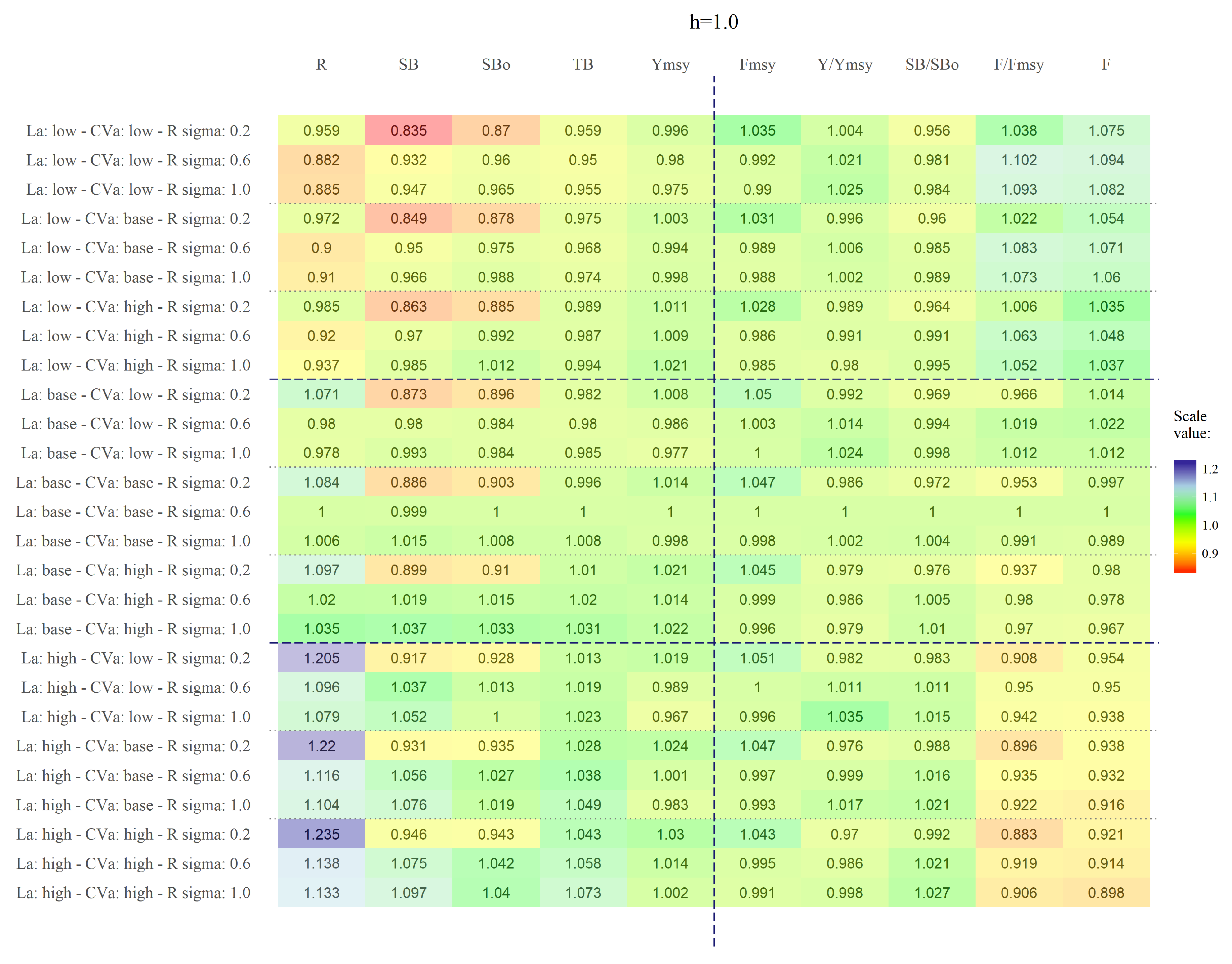
The effect of the changes in $L_{a=1}$, $c{v}_a$ and ${\sigma }_R^2$ on the stock assessment and management variables for $h=1$ are summarised in Figure 2 (left panel). The highest impact stems from changes in the parameter $L_{a=1}$ in comparison to changes in $c{v}_a$ or ${\sigma }_R^2$. Recruitment was the most affected variable in the stock assessment. In all scenarios, variations of $L_{a=1}$ lead to increases and reductions of R. Deviation of R compared to the base case scenario were close to a 24% maximum when $L_{a=1}$ was high and 11% when $L_{a=1}$ was low. The assessment variables $SB$, $S{B}_0$ were less impacted compared to R with a variation of 16.5% maximum and near 13% respectively when $L_{a=1}$ was low. A maximum of 10% ($SB$) and 6.5% ($S{B}_0$) were registered when $L_{a=1}$ was high. The assessment variables $TB$ and $Y_{MSY}$ were less affected across different scenarios of $L_{a=1}$, $c{v}_a$ and ${\sigma }_R^2$ (Figure 2).

Regarding the management variables for $h=1$, Figure 2 (right panel) the highest impact arisen from changes in $L_{a=1}$ and to a lesser extent from $c{v}_a$ or ${\sigma }_R^2$. Variations in $L_{a=1}$ between −10% (low) and +10% (high) (Figure 2) affected mainly the F and the ratio of $F/F_{MSY}$. The maximum variation in F was near to 9%, and 9.5% in $F/F_{MSY}$ when $L_{a=1}$ was high, and a maximum of 9.3% in F and $F_{MSY}$ when $L_{a=1}$ was low. Management variables, $F_{MSY}$ and $Y/Y_{MSY}$ showed less variations in most scenarios of $L_{a=1}$ and $c{v}_a$ with a maximum of a 5% and 3.5% respectively. Figure 2 shows little variation of $SB/S{B}_0$ with maximum near 4.5% across all scenarios.

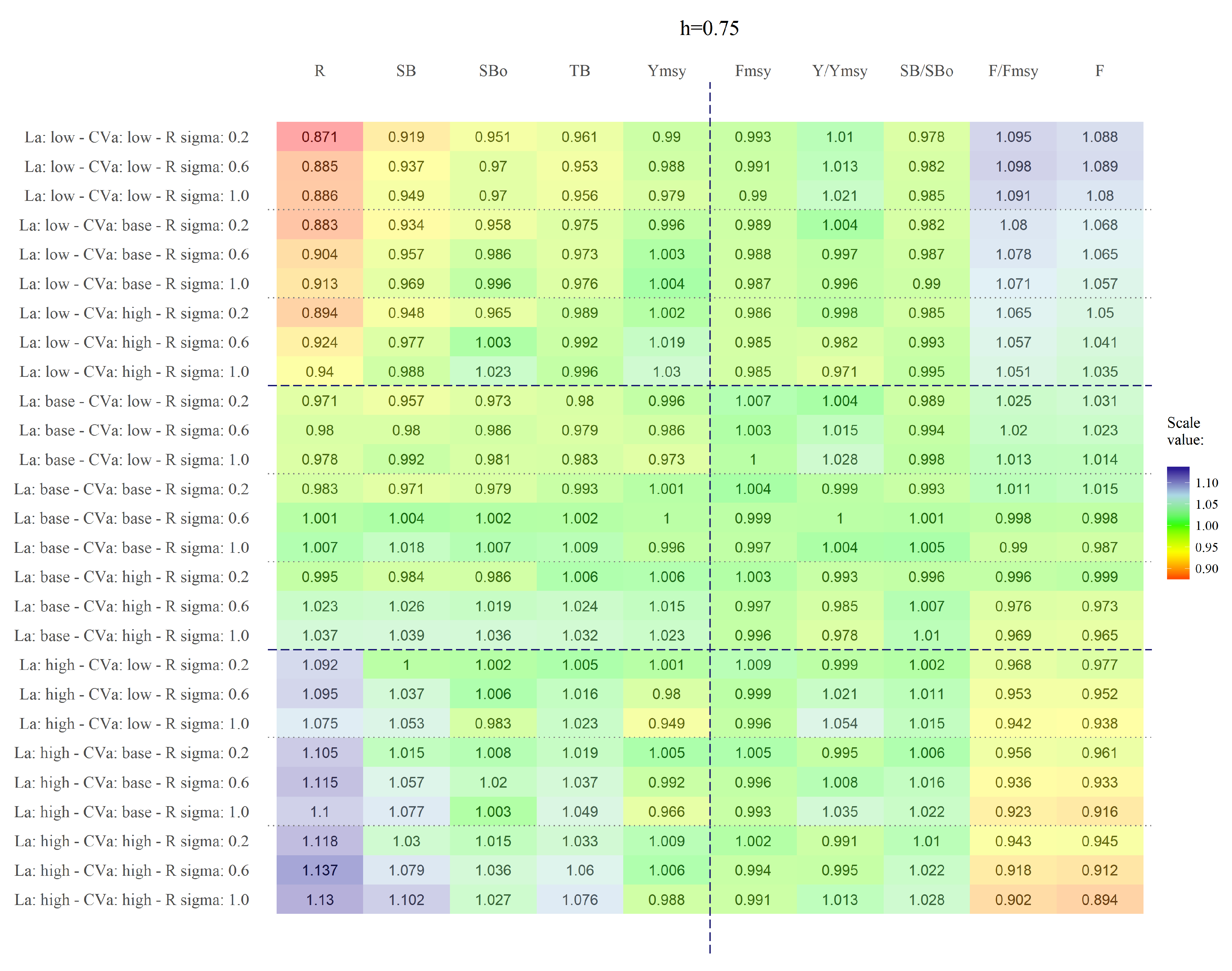
Figure 3 summarised the results of the combination of nine scenarios of variation in $L_{a=1}$, $c{v}_a$ and ${\sigma }_R^2$ for $h=0.75$. The impact of the changes on h, ${\sigma }_R^2$ and $c{v}_a$ on the stock assessment and management variables are negligible compared to the effect of the change in $L_{a=1}$ (Figure 3, left panel). As the same as the case of h = 1 the most impacted stock assessment variable in $h=0.75$ were R followed by $SB$. Variation in R variable when $L_{a=1}$ was low reached a maximum of 13%, instead when $L_{a=1}$ was high the maximum variation was near to 14% (Figure 3). In the case of $SB$ the maximum variation was near to a 10% when $L_{a=1}$ was high (Figure 3).

As well as in h = 1, management variables most affected were F and the ratio of $F/F_{MSY}$ with variations of a maximum of 9% and 10% respectively, whether $L_{a=1}$ was high or low. $F_{MSY}$, $SB/S{B}_0$ and $Y/Y_{MSY}$ were much less affected (bellow to a 5%) by the different scenarios compared to F and $F/F_{MSY}$.

Comparing across values of h (Figure 2 and Figure 3), small changes were observed in the scenarios where the recruitment variance arise from a distribution with a ${\sigma }_R^2=0.6$ and h move from a value 0.75 (Figure 3) to 1 (Figure 2). A similar result was obtained when ${\sigma }_R^2=1.0$ and h changed from 1 (Figure 2) to 0.75 (Figure 3). The only exception to the previous results was found when the recruitment variation assumed a value of ${\sigma }_R^2=0.2$ and the steepness value changed from $h=1$ to $h=0.75$. In this last case, the stock assessment and management variables were more sensitive to the changes in steepness (Figure 2 and Figure 3).

3.2. Reliability of the Parameters Estimation

Table 7. Median values (MV) and coefficient of variation (CV) for all trials. All simulations were run with a recruitment variance of ${\sigma }_R^2=0.6$. Convergence of each trial estimation is registered as percentage (%).

	${\mathit{L}}_{\mathit{a}=1}$		${\mathit{cv}}_{\mathit{a}}$		h		Convergence
	MV	CV	MV	CV	MV	CV	%
Trial 1	0.11	0.04	0.07	0.02	0.14	0.11	46
Trial 2	0.09	0.04	0.03	0.02	—	—	100
Trial 3	−0.12	0.09	—	—	—	—	100
Trial 4	—	—	0.05	0.03	—	—	94

summarised the median relative bias (MV) between the estimated parameters and those used in the simulation. It also shows the coefficient of variation (CV) of the parameters that comes from the models with a reliable solution in the optimisation process. In Trial 1 (Table 7), where $L_{a=1}$, $c{v}_a$ and h parameters were estimated simultaneously, $L_{a=1}$ and h show a biased estimation, because differences between simulated and estimated parameters were the largest. In addition, parameter h shows the highest variability with a CV equal to 0.11. When the simulation was focused on the growth parameters (Table 7, Trial 2), the reliability of the estimation increased, because the MV of $L_{a=1}$ and $c{v}_a$ are reduced, as well as the CV.

The higher reliability of the parameters estimated in the Trial 2 was also supported by the percentage of convergence equivalent to 100%. Indeed, when all parameters were estimated simultaneously (Table 7, Trial 1) the percentage of convergence was lower (46%) compared to the trial in which only growth parameters were estimated with a convergence level of 100% (Table 7, Trial 2). When $L_{a=1}$ was estimated alone (Table 7, Trial 3), also reveals less confidence in the estimation, the differences between the estimated and simulated parameters was MV = −0.12. The negative value arise from a 10% reduction in the parameter $L_{a=1}$, in this case the model estimated larger values for $L_{a=1}$. Thus, the $c{v}_a$ was the most reliable and precise parameter estimated in at least 94% of the runs, with the lower bias level (MV) and variability (CV) (Table 7, Trial 4). As expected, the estimation $L_{a=1}$ showed the highest bias and variability (Table 7, Trial 3) due to the largest impact on the stock assessment and management variables as shown in Section 3.1.

4. Discussion

We have shown that the length at first capture, $L_{a=1}$, has the highest impact on yellow squat lobster assessment and management variables. The variation of this parameter mainly affects recruitment (R) and secondarily, spawning biomass. Although, the other status variables were also affected, their variation was negligible. Contrary to our expectations, changes in the h assumption of the SRR and the variability of the recruitments (${\sigma }_R^2$) had a negligible impact on the studied variables. Changes in $L_{a=1}$ led to changes in individual mean weight, thus affecting directly the estimation of biomass and therefore the recruitments. Because the effects of the changes in h and ${\sigma }_R^2$ were negligible, we concluded that the shape and variability of the SRR do not have a major impact on the assessment and management variables. Therefore, observed variations in the amount of recruitment were mainly caused by changing in the spawning biomass triggered by different values of $L_{a=1}$.

Fishing mortality (F) and the ratio $F/F_{MSY}$ were the most affected management variables in all scenarios. However, when we analysed the effect of $F_{MSY}$ isolated; negligible variation arose across different scenarios for $L_{a=1}$, $c{v}_a$, h and ${\sigma }_R^2$. Thus, variations in $F/F_{MSY}$ are down to changes in F across scenarios. Variability in F was a consequence of changes in $L_{a=1}$ across scenarios that triggered changes in vulnerable biomass. This imply that $L_{a=1}$ could significantly affect the exploitation status perceived in yellow squat lobster. Variation in steepness (h) became relevant only when ${\sigma }_R^2=0.2$. Under such condition, low variation of recruitment estimates around the theoretical curve is allowed, and thus steepness becomes more relevant in determining the population renewal therefore triggering variations in population abundance.

$L_{a=1}$ was the most biased parameter estimated in the simulation analysis. The bias on $L_{a=1}$ increased when $c{v}_a$ remain fixed on the simulations in the estimation model, suggesting that the high correlation between these two parameters is important to maintain at least consistency on the estimation. $L_{a=1}$ is assumed constant across time, but observed length structures show high variations. Therefore, processes such as selectivity, growth parameters and recruitment need to vary across time to cope with observed variations on length structures. Indeed, when trying to estimate growth and recruitment parameters simultaneously, a poor optimisation process was reported (e.g., non-invertible Hessian matrix). This agrees with previous investigations suggesting that a confounding effect is found when estimating at the same time life history and recruitment parameters on integrated stock assessment models [11].

We propose that variations in $L_{a=1}$ have a major impact on the assessment and management variables of Chilean yellow squat lobster. This agrees with other works stating that misspecification of growth can result in deep uncertainties in parameter and management quantity estimates when the stock assessment models are fit to length structure [3]. The assessment framework of the yellow squat lobster depends on known growth parameter k and $L_{\infty }$, leading to fixed values of $L_{a=1}$ and $c{v}_a$. This issue calls for caution because it may give a false sense of certainty about the exploitation status of this species. As with many other crustacean species, direct observation of ages in yellow squat lobster is difficult. In Chile, age estimations used in stock assessments come exclusively from age distribution mixtures using length structures [12]. This method involves high levels of uncertainty because the numbers of age groups are essentially a subjective decision [7]. Yellow squat lobster showed wide variability on reported growth parameters across different studies [6,13,14,15,16]. Number of age groups assigned on the observed length structures varies from 5 [13,15] to 11 [6]. These variations in age groups assigned are then propagated into the estimated growth parameters. Values of k varied from 0.154 to 0.196 [year ${}^{-1}$] in females, and 0.118 to 0.221 [year ${}^{-1}$] in males. Additionally, $L_{\infty }$ takes values in the range of 45.6 to 54.6 [cm] in females and 52.8 to 62.1 [cm] in males. For current stock assessment in Chilean yellow squat lobster, selected beforehand, a set of fixed growth parameters and no further or formal sensitivity analysis is performed. Given the importance of the growth parameters on $L_{a=1}$ and $c{v}_a$ and therefore for the assessment and management variables of yellow squat lobster, we recommend to developing workable protocols that deal with these shortcomings. Alternatively, growth parameters could be estimate within the stock assessment model, thus including growth parameters and associate uncertainty as additional information to the integrated model [3]. Further work should includes extensive sensitivity analysis on how growth parameters are affected by selectivity, and how intermediate and old ages are affected by changes $L_{a=1}$. This also should be extended to the perception of status, since F was the variable most impacted by changes in $L_{a=1}$. In addition, others simulation scenarios could include a wider interval of values h since the value used here and in the stock assessment (h = 1) is at the boundary of the parameters space for h and this sometime could influencing the Hessian estimation.

During 2014, the Instituto de Fomento Pesquero (IFOP) conducted a project on biological reference points in Chilean fisheries subjected to annual quotas [9]. The project included extensive work, to classify stocks in tiers (groups) according to quantity and quality of the data available (poor, moderate, and rich data) and the reliability of the assessment estimates. Later, specific methods were proposed to estimate MSY-based RPs in each tier. Demersal crustacean fisheries, including yellow squat lobster, were classified in such tier in which proxy variables are used to estimate MSY- based RPs. This means that yellow squat lobster contains enough information to conduct an age-structured stock assessment, but h cannot reliably be estimated within the stock assessment model. Thus, simulation results presented here should be seen as complementary to the simulations analysis developed for MSY-based RPs [9]. Additionally, the simulation findings here suggest that in the process of parameterising the Chilean yellow squat lobster, the stock assessment model serves best to avoid the combined estimation of the parameters that describe the growth process and the stock-recruitment relationship. If the combined estimation is avoided, the bias in the estimation of the stock assessment and management variables will decrease.

We conclude that the parameters related to individual growth are the most important in determining the exploitation status of this stock. In an age-structured model where the fitted observed length structures show high inter-annual variability, an unbiased estimation of $L_{a=1}$ is very important. Thus, we recommend the use of workable simulation protocols for growth when using an age-structured model fitting length observations such as yellow squat lobster in Chile. The analysis was focused on the Northern stock of the Chilean yellow squat lobster, however our findings extend to all Chilean fisheries using age-structured models fitting length observations, because they shared the same assessment framework.

References

1. Wiff, R.; Quiroz, J.C.; Neira, S.; Gacitúa, S.; Barrientos, M.A. Chilean Fishing Law, Maximum sustainable Yield and the Stock-Recruitment relationship. Lat. Am. J. Aquat. Res. 2016, 44, 380–391. [Google Scholar] [CrossRef]
2. Punt, A.E.; Huang, T.; Maunder, M.N. Review of integrated size-structured models for stock assessment of hard-to-age crustacean and molluscum species. ICES J. Mar. Sci. 2013, 70, 16–33. [Google Scholar] [CrossRef] [Green Version]
3. Aires-da-Silva, A.M.; Maunder, M.N.; Schaefer, K.M.; Fuller, D.W. Improved growth estimates from integrated analysis of direct aging and tag–recapture data: An illustration with bigeye tuna (Thunnus obesus) of the eastern pacific ocean with implications for management. Fish. Res. 2015, 163, 119–126. [Google Scholar] [CrossRef]
4. Mace, P.M.; Doonan, I.J. A Generalized Bioeconomic Simulation Model for Fish Dynamics; New Zealand Fishery Assessment Research Document 88/4; NZ Ministry of Agriculture and Fisheries: Wellington, New Zealand, 1988; 51p.
5. Bucarey, D.; Cavieres, J.; Montenegro, C.; Zilleruelo, M.; Párraga, D.; Bravo, C. Investigación del status y posibilidades de explotación biológicamente sustentables en langostino amarillo, año 2015; Informe Consolidado; Subsecretaria de Pesca—Instituto de Fomento Pesquero: Valparaíso, Chile, 2015; 94p. [Google Scholar]
6. Arancibia, H.; Cubillos, L.A.; Acuña, E. Annual growth and age composition of the squat lobster Cervimunida johni off northern-central Chile (1996–97). Sci. Mar. 2005, 69, 113–122. [Google Scholar]
7. Roa-Ureta, R. A likelihood-based model of fish growth with multiple length frequency data. J. Agric. Biol. Environ. Stat. 2010, 15, 416–429. [Google Scholar] [CrossRef]
8. Mangel, M.; Brodziak, J.; DiNardo, G. Reproductive ecology and scientific inference of steepness: A fundamental metric of population dynamics and strategic fisheries management. Fish Fish. 2010, 11, 89–104. [Google Scholar] [CrossRef]
9. Payá, I.; Canales, C.; Bucarey, D.; Canales, T.M.; Contreras, F.; Leal, E.; Tascheri, R.; Yáñez, A.; Zúñiga, M.J.; Clark, W.; et al. Revisión de los Puntos Biológicos de Referencia (Rendimiento Máximo Sostenible) en las Pesquerías Nacionales; Tercer Reporte Técnico; Instituto de Fomento Pesquero: Valparaíso, Chile, 2014; 51p. [Google Scholar]
10. Fournier, D.A.; Skaug, H.J.; Ancheta, J.; Ianelli, J.; Magnusson, A.; Maunder, M.N.; Nielsen, A.; Sibert, J. AD Model Builder: Using automatic differentiation for statistical inference of highly parameterized complex nonlinear models. Optim. Methods Softw. 2012, 27, 233–249. [Google Scholar] [CrossRef] [Green Version]
11. Lee, H.H.; Maunder, M.N.; Piner, K.P.; Method, R.D. Can steepness of the stock-recruitment relationship be estimated in fishery stock assessment models? Fish. Res. 2012, 125–126, 254–261. [Google Scholar] [CrossRef]
12. MacDonald, P.D.M.; Pitcher, T.J. Age groups from size-frequency data: A versalite and efficient method for analyzing distribution mixtures. Can. J. Fish. Aquat. Sci. 1979, 36, 987–1001. [Google Scholar] [CrossRef]
13. Pavéz, P.; Peñailillo, T.; Palma, M.; Silva, N.; Miranda, H.; Giakoni, I. Evaluación directa del stock de Langostino amarillo en la zona centro-norte; Informe Final, Fondo de Investigación Pesquera Nro. 93-06; Pontificia Universidad Católica de Valparaíso: Valparaíso, Chile, 1994; 132p. [Google Scholar]
14. Pavéz, P.; Falcón, C. Crecimiento, mortalidad y función de stock en el langostino amarillo (Cervimunida johni) entre Valparaíso (V Región) y Talcahuano (VIII Región); Documento Técnico Nro. 48-95; Pontificia Universidad Católica de Valparaíso: Valparaíso, Chile, 1995; 40p. [Google Scholar]
15. Pool, H.; Canales, C.; Montenegro, C. Evaluación del Recurso Langostino amarillo en la Zona Centro Norte; Informe Final, Fondo de Investigación Pesquera Nro. 94-25; Instituto de Fomento Pesquero: Valparaíso, Chile, 1996; 55p. [Google Scholar]
16. Acuña, E.; Arancibia, H.; Mujica, A.; Cid, L.; Roa, R. Análisis de la pesquería y Evaluación indirecta del stock de langostino amarillo en la III y IV Regiones; Informe Final, Fondo de Investigación Pesquera Nro. 96-08; Universidad Católica del Norte: Coquimbo, Chile, 1996; 153p. [Google Scholar]
Figure 1. Distribution of the yellow squat lobster off the Chilean coast in shaded area. Dashed line indicates the division of stocks: Northern stock distributed between 26 03 S–30 30 S and the Southern stock between 30 30 S -38 48 S.
Jmse 08 00423 g001
Figure 2. Assessment and management variables results for each scenario that combine Table 4 and Table 5 for an steepness value of h = 1. Left white column show each scenario of mean length at first capture L a = 1 (low (−10%), base (base case scenario), high (+10%)), coefficient of variation at age c v a (low (−10%), base, high (+10%)) and recruitment variability σ R 2 (0.2, 0.6 and 1). Assessment variables correspond to R (average recruitment), S B (spawning biomass in the last year), S B 0 (unfished spawning biomass), T B (Total biomass), Y M S Y (catch at the maximum sustainable yield, M S Y ). Management variables were F M S Y (target fishing mortality), Y / Y M S Y (ratio between last year yield (Y) and yield at M S Y ), S B / S B 0 (ratio between the S B in the last year and the unfished spawning biomass), F / F M S Y (ratio between the fishing mortality in the last year (F) and fishing mortality at M S Y ) and F. Value equals 1 indicates no change regarding the base case scenario.
Jmse 08 00423 g002
Figure 3. Assessment and management variables results for each scenario that combine Table 4 and Table 5 for an steepness value of h = 0.75. Left white column show each scenario of mean length at first capture L a = 1 (low (−10%), base (base case scenario), high (+10%)), coefficient of variation at age c v a (low (−10%), base, high (+10%)) and recruitment variability σ R 2 (0.2, 0.6 and 1). Assessment variables correspond to R (average recruitment), S B (spawning biomass in the last year), S B 0 (unfished spawning biomass), T B (Total biomass), Y M S Y (catch at the maximum sustainable yield, M S Y ). Management variables were F M S Y (target fishing mortality), Y / Y M S Y (ratio between last year yield (Y) and yield at M S Y ), S B / S B 0 (ratio between the S B in the last year and the unfished spawning biomass), F / F M S Y (ratio between the fishing mortality in the last year (F) and fishing mortality at M S Y ) and F. Value equals 1 indicates no change regarding the base case scenario.
Jmse 08 00423 g003