Numerical Simulation and Validation in Scrubber Wash Water Discharge from Ships

Abstract

A regulation on the sulfur emissions of ships sailing in global sea areas has been enforced since 1 January 2020. In this new regulation, ships are required to use low-sulfur fuel oils or to install an after-treatment equipment, such as a scrubber. Open and hybrid scrubbers wash the exhaust gas using seawater and then discharge the wash water overboard. According to the regulation promulgated by the International Maritime Organization (IMO) Marine Environment Protection Committee (MEPC), the wash water must have a pH of 6.5 or higher at 4 m from the discharge point. Wash water is generally acidic, with a pH of 2.5–3.5, whereas seawater is alkaline, with a pH of approximately 8.2. The wash water is dispersed after being discharged overboard through a nozzle, and its pH is restored through dilution with the surrounding seawater. In this study, the pH was calculated by using a theoretical chemical reaction model, and then the dispersion of wash water was analyzed using CFD simulation. This study describes the process of selecting the appropriate turbulent Schmidt number in a wide range of nozzle diameters. Finally, the appropriate nozzle diameter was determined based on the initial pH of the discharged scrubber wash.

1. Introduction

In January 2020, the International Maritime Organization (IMO) enforced a regulation stipulating that the sulfur content of fuel used by ships sailing in the global sea area should be reduced from 3.5% to 0.5% [1,2]. In the future, it is expected that much attention will be given on regulations on emissions from ships. Shipping companies have searched for measures to comply with this new regulation on SOx emission. The most popular measure is the use of low-sulfur fuel oil (LSFO). For most ships that do not use LSFO, a scrubber was installed instead to remove SOx. Besides using LSFO or a scrubber, another option is to use alternative fuels, such as liquefied natural gas [3,4].

A scrubber is a washing system for exhaust gas. Scrubbers are classified into open-loop system, closed-loop system, and hybrid system, which combines the first two systems [5]. The open-loop system washes the exhaust gas using alkaline seawater and discharges the wash water overboard. This system has the simplest structure and is the most advantageous in terms of economic operation cost compared with the other types of scrubber [6]. The closed-loop system washes the exhaust gas using fresh water and then recycles the wash water using NaOH. The open-loop system and the hybrid system wash the exhaust gas using seawater, and discharge the wash water off-board because it is difficult to keep a large volume of wash water on-board.

However, there has been a discussion on the harmful effects of scrubber wash water [7,8], and some European sea areas and U.S. coastal areas prohibit the discharge of scrubber wash water. The number of sea areas where the discharge of scrubber wash water is restricted may increase in the future. Thus, shipping companies must install a closed-loop system scrubber or a hybrid scrubber to comply with the SOx regulations; when they opt to use an open-loop scrubber system, they must use LSFO in sea areas where wash water discharge is restricted.

The current regulations stipulate that when stationary ships discharge scrubber wash water, the wash water at 4 m from the discharge point must have a pH of 6.5 or higher. Compliance to this regulation must be verified through experiments or through other equivalent scientifically proven methods, including numerical analysis, and must be certified by a classification society. Then the report must be kept on board [1].

Üplre et al. [9] theoretically and experimentally investigated the discharge of acidic turbulent jets in an alkaline environment. Their chemical model matched well with their titration experiment results. They introduced an empirical model of turbulent jets and integrated it with chemistry and fluid flow models. Also, Ülpre and Eames [10] conducted a physical and chemical research on the discharge of scrubber wash water from ships. To comply with the IMO’s regulation on scrubber wash water discharge from ships, they developed a procedure for the use of multiple ports.

Turbulent jets have long been investigated because they are applied in various industries [11,12,13]. Studies in this field mainly focused on the velocity and concentration distributions of turbulent jets. With the development of numerical analysis, efforts have been made to match the experimental values with numerical analysis results. Pani et al. [14] proposed a point-source method to predict the velocity field of turbulent jets, and they found that their result agreed well with the CFD simulation. By considering the effect of buoyancy, Robinson et al. [15] conducted a numerical analysis on the mixing and dispersion of turbulent jets. They performed CFD simulation of two cases, namely, horizontal and angled jets, and then compared their result with published experimental results. In their numerical analysis, they applied the k-ε turbulence model and the Smagorinsky LES model, and they used adaptive mesh. Different results were obtained depending on the mesh quality. The simulation predicted the buoyant jet well, but it overestimated dispersion in a near field of the source.

Choi et al. [16] determined, through CFD, the discharge velocity and dilution ratio under different discharge velocities and nozzle diameters. The discharge velocity from the turbulent jets exerted little effect on dilution. However, in the study, the CFD validation process was insufficient, so the dilution ratio according to the nozzle diameter seems to have a low reliability.

In this study, the pH according to the dilution ratio of wash water and seawater was calculated through a theoretical chemical reaction model, and the volume fraction of wash water in the wash water-seawater mixture was calculated through CFD simulation. In addition, the pH was calculated by combining the dilution ratio, which was calculated using the theoretical chemical reaction model, and the volume fraction that was determined through CFD simulation. Furthermore, this paper details the accurate simulation method for turbulent jet flow under various nozzle diameters. Generally, the simulation of two-phase flow is implemented by using mixture model or volume of fluid (VOF) model. These models require a lot of time to calculate and are difficult to validate. In this study, the process in which the scrubber wash water is discharged and dispersed into the sea water is simulated solving the transport equation, and this method is highly dependent on the turbulent Schmidt number. Although studies that investigated the effect of Schmidt number on the flow have already been published, it is difficult to find a study that increases the reliability of the analysis by selecting the appropriate turbulent Schmidt number in the field of ship’s scrubber technology. Therefore, we propose herein the use of appropriate turbulent Schmidt numbers according to the nozzle diameter. This study proposes an accurate and easy-to-access approach to calculate the pH of scrubber wash water discharged from ships. Results of this study are expected to be useful to scrubber manufacturers, to ship-building companies, and to classification societies.

2. Theoretical Analysis

2.1. Chemistry Reaction

In this study, modeling was based on the acid-weak alkali reaction reported in the works of Ülpre et al. [9] and Ülpre [17]. These chemical reactions are detailed in said references. Seawater is a weak base buffer solution. A buffer solution is a solution that absorbs hydrogen ions even when a small amount of acid is added and thus causes almost no change in pH. The buffer capacity of seawater is mainly determined by the $HC{O}_3^{-}$ and $C{O}_3^{2-}$ ions [9,18].

The chemical equilibrium of the acid HA and the base MOH is expressed as follows:

$$\left[H^{+}\right]+\left[M^{+}\right]=\left[O{H}^{-}\right]+\left[A^{-}\right]$$

(1)

The mass of acid (a) and base (b) are conserved by Equations (2) and (3):

$$C_a{V}_a=\left[A^{-}\right]\left(V_a+V_b\right)$$

(2)

$$C_b{V}_b=\left(\left[MOH\right]+\left[M^{+}\right]\right)\left(V_a+V_b\right)$$

(3)

where C indicates concentration and V indicates volume.

When Equation (1) is substituted in Equation (2), the following equation is obtained:

$$C_a{V}_a=\left(\left[H^{+}\right]+\left[M^{+}\right]-\left[O{H}^{-}\right]\right)\left(V_a+V_b\right)$$

(4)

Furthermore, when Equation (4) is substituted in Equation (3), Equation (5) is obtained, and Equation (5) can be summarized as Equation (6).

$$C_b{V}_b=\left(\left[MOH\right]+\frac{C_a{V}_a}{V_a+V_b}-\left[H^{+}\right]+\left[O{H}^{-}\right]\right)\left(V_a+V_b\right)$$

(5)

$$V_a\left(C_a-\left[H^{+}\right]+\left[O{H}^{-}\right]\right)=V_b\left(C_b+\left[H^{+}\right]-\left[O{H}^{-}\right]\right)-\left[MOH\right]\left(V_a+V_b\right)$$

(6)

The ionization constants of water, acid, and base are defined as follows:

$$K_w=\left[O{H}^{-}\right]\left[H^{+}\right]$$

(7)

$$K_a=\frac{\left[H^{+}\right]\left[A^{-}\right]}{\left[HA\right]}$$

(8)

$$K_b=\frac{\left[M^{+}\right]\left[O{H}^{-}\right]}{\left[MOH\right]}=\frac{K_w}{K_a}$$

(9)

When Equation (9) is substituted in Equation (3), the following equation is obtained:

$$\left[MOH\right]\left(V_a+V_b\right)=C_b{V}_b-\left(\frac{C_b{V}_b}{\frac{\left[OH\right]}{K_b}+1}\right)$$

(10)

When Equations (10) and (8) are substituted in Equation (6), the following standard acid-alkali titration equation is obtained:

$$\frac{V_b}{V_a}=\frac{C_a-\left[H^{+}\right]+\frac{K_w}{\left[H^{+}\right]}}{\frac{C_b}{1+K_w/\left(\left[H^{+}\right]K_b\right)}+\left[H^{+}\right]-\frac{K_w}{\left[H^{+}\right]}}$$

(11)

In weak base reaction, Equation (11) can be expressed as:

$$\frac{V_b}{V_a}=\frac{C_a-\left[H^{+}\right]+\frac{K_w}{\left[H^{+}\right]}}{\frac{C_b{K}_b}{K_w/\left[H^{+}\right]}+\left[H^{+}\right]-\frac{K_w}{\left[H^{+}\right]}}\mathrm{for}\frac{K_w}{\left[H^{+}\right]}\gg K_b$$

(12)

In addition, the reaction of diprotic acid can be expressed as:

$$\frac{V_b}{V_a}=\frac{\frac{C_a\left(K_{a1}\left[H^{+}\right]+2K_{a1}{K}_{a2}\right)}{\left({\left[H^{+}\right]}^2+K_{a1}\left[H^{+}\right]+K_{a1}{K}_{a2}\right)-\left[H^{+}\right]+K_w/\left[H^{+}\right]}}{\frac{C_b}{\left(1+K_w/\left(\left[H^{+}\right]K_b\right)\right)}+\left[H^{+}\right]-K_w/\left[H^{+}\right]}$$

(13)

The constants used in this study are as follows [9,19]: $K_w={10}^{-14}$, $K_{a1}=1$, $K_{a2}=1.2\times {10}^{-2}$, $K_b=2.3\times {10}^{-8}$. $K_w$ is the ionization constant of water, $K_{a1}$, $K_{a2}$ and $K_b$ are the ionization constants of H₂SO₄ and HCO₃⁻, respectively.

2.2. Turbulent Jets

Pani et al. [14] proposed the following velocity distribution correlation and concentration distribution correlation in circular turbulent jets:

$$\frac{u}{u_0}=6.2{\left(\frac{Z}{D}\right)}^{-1}$$

(14)

$$\frac{C}{C_0}=5.26{\left(\frac{Z}{D}\right)}^{-1}$$

(15)

where u is the velocity; u₀ is the initial velocity at the discharge point; Z and D denote the axial distance and nozzle diameter, respectively; and C and C₀ denote the concentration and initial concentration at the discharge point, respectively.

Furthermore, Hodgson et al. [20] suggested the following concentration distribution correlation in circular turbulent jets:

$$\frac{C}{C_0}=5.34{\left(\frac{Z}{D}\right)}^{-1}$$

(16)

Equation (16) predicts a higher concentration than Equation (15), and a higher concentration indicates poor dilution. Thus, we adopted harsh conditions to minimize risks in this study. To verify the numerical analysis results, we compared the numerical analysis result with Equation (16).

3. Numerical Modeling

Using the chemical reaction model described in Section 2, the pH based on the dilution ratio of wash water and seawater can be calculated. Hence, the dilution ratio can be calculated by analyzing wash water dispersion without considering the chemical reaction in the numerical analysis. In the present study, CFD simulation was performed to simulate the discharge and dispersion process of wash water in seawater. Since the chemical reaction between wash water and seawater was assumed to occur within a considerably short period of time (10⁻⁹ s) compared with the physical mixing process [21], it was assumed that the chemical reaction does not affect the physical mixing. In addition, since the wash water is mostly composed of seawater, we used the properties of the latter. However, wash water and seawater are assumed to be totally different fluids, and the concentration of wash water was calculated in the same manner as the volume fraction of wash water. In this study, the commercial code ANSYS-CFX V13.0 was used for CFD simulation.

Since many studies have already reported that the k-ε model is appropriate for flow analysis in order to simulate turbulent jets [15,22,23], our study also used the k-ε model. In this model, $k$ and $\epsilon$ are expressed in their respective transport equations as follows [23,24]:

$$\frac{\partial }{\partial x_j}\left(\rho u_{j}k\right)=\frac{\partial }{\partial x_j}\left[\left(\mu +\frac{{\mu }_t}{{\sigma }_k}\right)\frac{\partial k}{\partial x_j}\right]+P_k-\rho \epsilon +P_{kb}$$

(17)

$$\frac{\partial }{\partial x_j}\left(\rho u_j\epsilon \right)=\frac{\partial }{\partial x_j}\left[\left(\mu +\frac{{\mu }_t}{{\sigma }_{\epsilon }}\right)\frac{\partial \epsilon }{\partial x_j}\right]+\frac{\epsilon }{k}\left(C_{\epsilon 1}{P}_k-C_{\epsilon 2}\rho \epsilon +C_{\epsilon 1}{P}_{\epsilon b}\right)$$

(18)

$P_{kb}$ is defined by an equation for $S{c}_t$, as follows:

$$P_{kb}=\frac{{\mu }_t}{S{c}_t}\beta g_i\frac{\partial T}{\partial x_i}$$

(19)

where $k$ and $\epsilon$ denote the turbulence kinetic energy and turbulence eddy dissipation, respectively; ${\mu }_t$, $\beta$, and $g_i$ denote the turbulence viscosity, thermal expansion coefficient, and gravity vector, respectively. The constant values are as follows: $C_{\epsilon 1}=1.45, C_{\epsilon 2}=1.9$, ${\sigma }_k=1.0$, ${\sigma }_{\epsilon }=1.3$.

Here, $S{c}_t$ is a turbulent Schmidt number, and the default value provided by ANSYS-CFX is 0.9. $S{c}_t$ is a major parameter that affects dispersion in the k-ε turbulence simulation [22,25] and is mainly obtained experimentally. Oliver et al. [22] suggested that $S{c}_t$ is approximately 0.7 when buoyancy is not considered, whereas it is 0.6 when buoyancy is considered. However, the appropriate $S{c}_t$ value is dependent on the nozzle diameter and shape and on the working fluid type. In this study, CFD was validated through the selection of the appropriate $S{c}_t$ which is dependent on the nozzle diameter.

The objective of CFD simulation was to verify the volume fraction, which changes according to the dispersion of wash water. Therefore, the transport equation was solved by applying the volume fraction to the transport equation, defined as Equation (20), by using the volume fraction (vf) as an additional variable without considering the complex detailed model of the two-phase flow [26]. The volume fraction of the wash water discharged from the nozzle was set as 1. Thus, the volume fraction of wash water in the initial external seawater of the nozzle is zero.

$$\frac{\partial \left(\rho vf\right)}{\partial t}+\nabla ·\left(\rho uvf\right)=\nabla ·\left(\left(\rho \alpha +\frac{{\mu }_t}{S{c}_{add}}\right)\nabla vf\right)+S$$

(20)

In Equation (20), $S{c}_{add}$, $\alpha$, and $S$ denote the turbulent Schmidt number, kinematic diffusivity, and source term of the additional variable, respectively.

3.1. Boundary Conditions

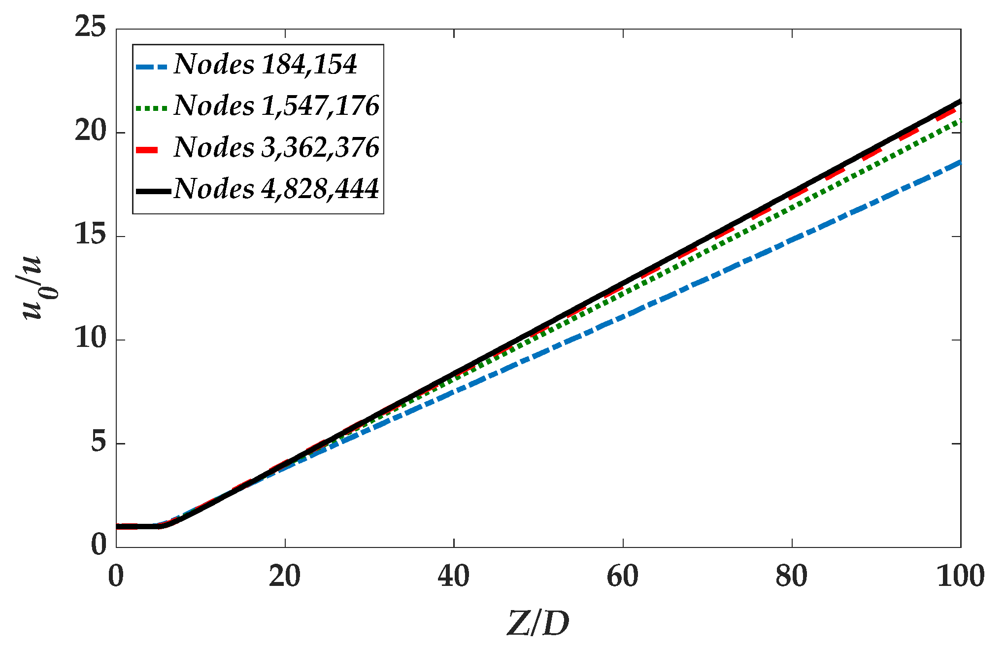
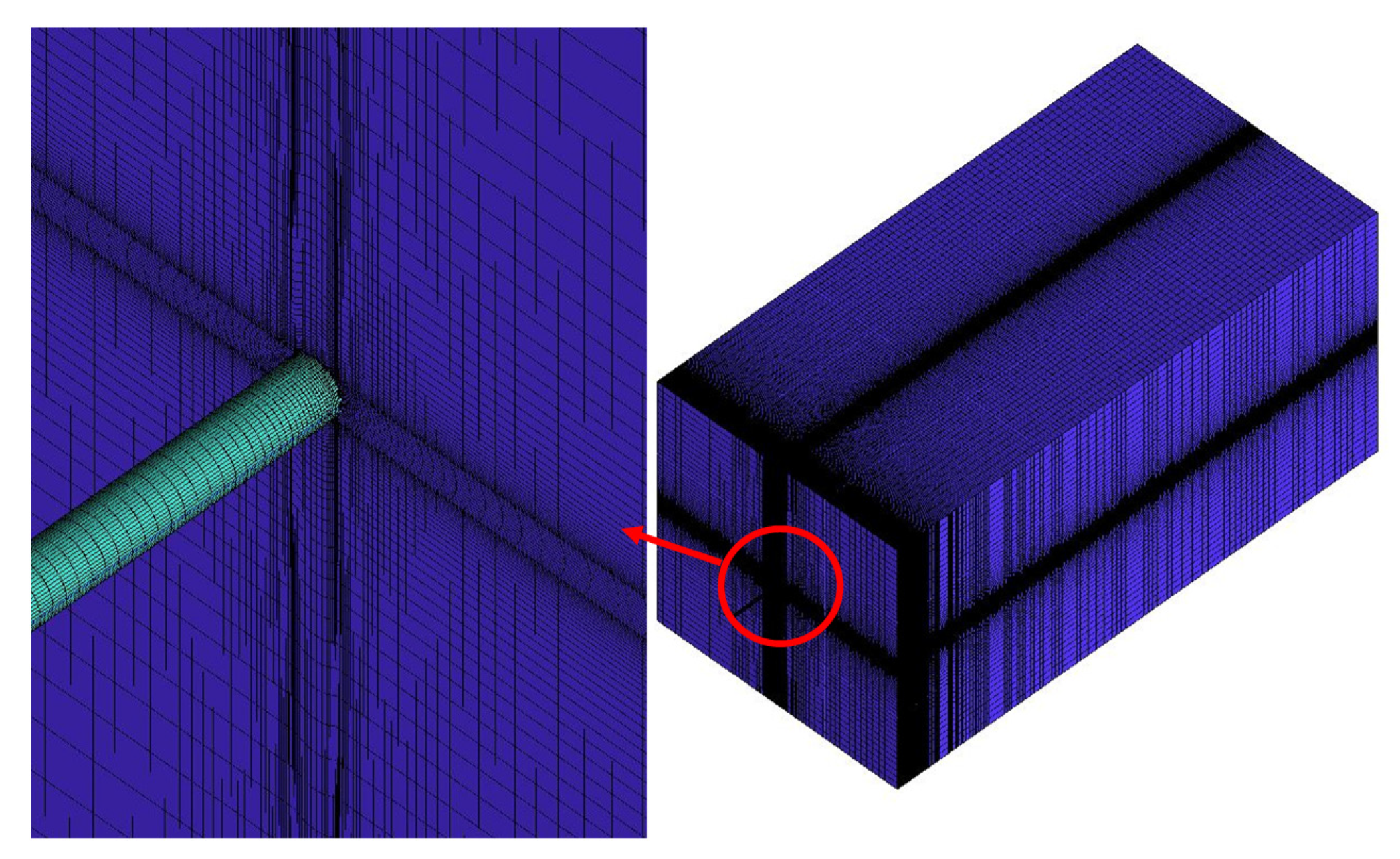
The nozzle length was set as 20 times the nozzle diameter to simulate the fully developed flow of wash water discharged from the nozzle. A study [16] showed that the discharge velocity from a turbulent jet flow exerts almost no effect on dilution. In the present study, the dispersion of wash water according to the change in nozzle diameter was verified through CFD, and the CFD model was validated based on the existing literature. For the CFD simulation, nozzles with a diameter of 0.05–0.40 m were used. The discharge velocity of wash water from the nozzle is 1 m/s, and the opening condition was used for the exterior of the total domain. In actual flows, buoyancy can be generated by the temperature and density differences between the wash water and seawater, but buoyancy was ignored in this study. Compared with the results of studies that considered buoyancy, the present result showed that risk was minimized because the prevailing condition within 4 m from the discharge point is disadvantageous for dilution.

3.2. Mesh

The quality of mesh used in CFD numerical analysis exerts a decisive effect on the result. In this study, hexahedral meshes were generated using ANSYS ICEM-CFD. Dense meshes were generated using the O-grid method for areas where the gradient of velocity and transport variables were expected to be large. In addition, mesh dependence was reviewed using approximately 180,000, 1.5 million, 3.3 million, and 4.8 million nodes for a nozzle diameter of 0.05 m.

Figure 1 shows the dimensionless velocity according to the axial distance of discharge for different numbers of nodes. Dimensionless velocity is the local velocity divided by the maximum velocity. As the distance from the discharge point increased, variation in the results also increased depending on the number of meshes. At the point where the wash water is discharged from the nozzle, a rapid velocity gradient occurs due to the interaction of the wash water with the surrounding stagnant fluid. Hence, a sufficient number of meshes is required to simulate the dispersion phenomenon in this area. Therefore, 4.8 million meshes were selected based on the nozzle diameter of 0.05 m in this study. Figure 2 shows the hexahedral meshes used in this study.

4. Results

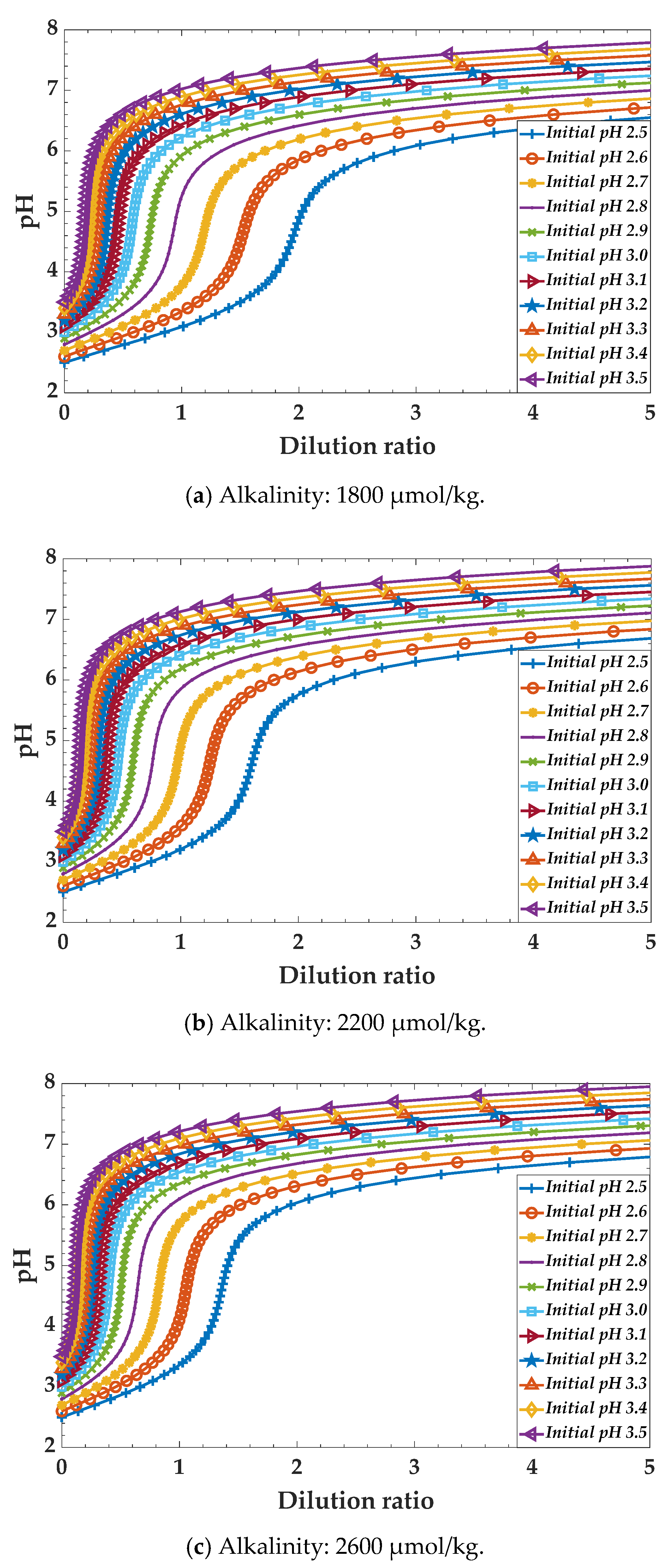
4.1. Titration Curves

Figure 3 shows the titration curves of the chemical reaction model described in Section 2.1; this model describes the variations in pH as a function of the dilution ratio ($V_b/V_a$) of wash water at an alkalinity of 1800, 2200, and 2600 μmol/kg, and at an initial pH of 2.5–3.5. When the seawater alkalinity was 2200 μmol/kg, the initial pH of 2.5 increased to 6.5 at a dilution ratio of approximately 3.81, and the initial pH of 3.5 increased to 6.5 at a dilution ratio of approximately 0.35.

Table 1. Required dilution ratio and volume fraction depending on the initial pH of scrubber wash water under different seawater alkalinity values.

Initial pH	Alkalinity 1800 μmol/kg		Alkalinity 2200 μmol/kg		Alkalinity 2600 μmol/kg
	Dilution Ratio	Volume Fraction	Dilution Ratio	Volume Fraction	Dilution Ratio	Volume Fraction
2.5	4.66	0.18	3.81	0.21	3.23	0.24
2.6	3.63	0.22	2.97	0.25	2.51	0.28
2.7	2.83	0.26	2.32	0.30	1.96	0.34
2.8	2.22	0.31	1.82	0.36	1.54	0.39
2.9	1.74	0.36	1.43	0.41	1.21	0.45
3.0	1.37	0.42	1.12	0.47	0.95	0.51
3.1	1.08	0.48	0.88	0.53	0.75	0.57
3.2	0.85	0.54	0.70	0.59	0.59	0.63
3.3	0.67	0.60	0.55	0.64	0.47	0.68
3.4	0.53	0.65	0.44	0.70	0.37	0.73
3.5	0.42	0.70	0.35	0.74	0.29	0.77

outlines the volume fractions ($V_a/\left(V_a+V_b\right)$) of the dilution ratio and wash water to achieve a pH of 6.5 based on the initial pH. When the seawater alkalinity was 1800 μmol/kg, dilution ratios of 4.66 and 0.42, respectively, should be provided for the initial pH 2.5 and 3.5 to be pH of 6.5. For the dilution ratios, 4.66 and 0.42 are converted to volume fraction of wash water of 0.18 and 0.70, respectively. When the seawater alkalinity was 2600 μmol/kg, the volume fractions of the wash water for the initial pH of 2.5 and 3.5 to be pH of 6.5 are 0.24 and 0.77 respectively. This means that a relatively large amount of sea water is required to recover the wash water to pH of 6.5 at low alkalinity compared to high alkalinity. On the other hand, a low initial pH of wash water requires a large amount of sea water to recover to pH of 6.5.

4.2. CFD Validations

Figure 4 shows the variations in the dimensionless velocity ($u_0/u$) according to Equation (14), which is the correlation reported by Pani et al. [14]; it also shows the change in $S{c}_t$. In Figure 4, the x-axis represents the dimensionless distance $\left(Z/D\right)$. Equation (14) is a simple model that has a linear relationship between the dimensionless velocity and the dimensionless distance. Therefore, it is not possible to make accurate predictions at the initial discharge, that is, at a low dimensionless distance. The results of CFD simulation can be compared to Equation (14) only in the region with linearity as the dimensionless distance increases. In this study, only the total length of 5 m was considered for analysis, because the focus is on the flow variable at the 4 m point. It can be seen that $S{c}_t$ is a major parameter in the turbulent jet flow. As $S{c}_t$ increased, the dimensionless velocity also increased, whereas the axial local velocity (u) decreased. At a diameter of 0.05 m, a $S{c}_t$ value of approximately 0.54 was found to match best with the correlation reported by Pani et al. [14]; at a diameter of 0.40 m, the $S{c}_t$ value of 0.75 matched best with the said correlation. Figure 5 shows the $S{c}_t$ values that match best with Pani et al.’s [14] correlation for each nozzle diameter. The nozzle diameter and $S{c}_t$ displayed a nearly linear relationship, which can be linearly interpolated as follows:

$$Sc=0.619D+0.5007$$

(21)

It should be noted that the $S{c}_t$ derived by Equation (21) is valid only when the working fluid is seawater, when the nozzle diameter is 0.05–0.40 m, and when the distance from the discharge point is less than 5 m.

Figure 6 shows the inverse of the volume fraction according to Equation (20), which is the correlation reported by Hodgson et al. [20]; it also shows the variation in $S{c}_{add}$. As with the above velocity distribution, only the total length of 5 m was considered for analysis. As the $S{c}_{add}$ increased, the inverse of volume fraction decreased, and the volume fraction increased. In other words, at low $S{c}_{add}$, dispersion and mixing actively occur. At a diameter of 0.05 m, the $S{c}_{add}$ of 0.71 matched best with the correlation reported by Hodgson et al. [20]; at a diameter of 0.40 m, the $S{c}_{add}$ of 0.63 matched best with the said correlation. Figure 7 shows the $S{c}_{add}$ values that match best with the correlation reported by Hodgson et al. [20] for each nozzle diameter. It can be linearly interpolated as follows:

$$S{c}_{add}=-0.238D+0.724$$

(22)

Finally, numerical analysis was performed by setting the optimal $S{c}_{add}$ for each nozzle diameter. Figure 8 shows the comparison between the volume fraction result of Hodgson et al. [20] at 4 m from the discharge point and the result of the numerical analysis. It was found that the numerical analysis result matched well with the result obtained by Hodgson et al. [20]. However, the $S{c}_t$ and $S{c}_{add}$ proposed in this study must be used under limited conditions. It should be noted that they are valid only when buoyancy is not considered, when the working fluid is seawater, when the nozzle diameter is 0.05–0.40 m, and when the distance from the discharge point is less than 5 m. The CFD post processing data is detailed in Appendix A.

The CFD results were compared with experimental data available in the literature for validation. Papanicolaou and List [27] conducted the experimental study on the vertical turbulent buoyant jets using lase-Doppler anemometry. They verified the velocity and concentration decay experimentally, and calculated the momentum fluxes using dimensionless parameters. Figure 9 shows the comparison between the CFD results and the experimental results obtained by Papanicolaou and List [27]. It was found that the simulation predicts well the results from Papanicolau and List [27].

4.3. pH Calculations

The volume fraction of wash water to achieve a pH of 6.5 in the wash water-seawater mixture can be determined based on the titration curves obtained in Section 4.1 and presented in Table 1. To achieve a pH of 6.5 by mixing with seawater that has an alkalinity of 2200 μmol/kg, a volume fraction of 0.21 is required when the wash water has an initial pH of 2.5, and a volume fraction of 0.74 is required when the initial pH is 3.5. The volume fraction at 4 m from the discharge point was calculated through the CFD numerical analysis described above.

Figure 10 shows the diameter required to achieve a pH of 6.5 at 4 m from the discharge point depending on the initial pH. Moreover, it shows the relationship between pH and nozzle diameter at different alkalinity values of seawater. At a low alkalinity, a large amount of seawater is required to restore the pH of the wash water, so the nozzle diameter must be small to facilitate dispersion. The nozzle diameter should be less than 0.34 m at the initial pH of 3.0 and alkalinity of 2200 μmol/kg and less than 0.30 m at alkalinity of 1800 μmol/kg to satisfy the regulation. Scrubber manufacturers can measure the pH of wash water and can roughly calculate the nozzle diameter for wash water discharge, based on the information shown in Figure 10. If the diameter is too small to discharge enough wash water, multiple ports should be considered. The wash water discharged from multiple ports should not interfere with each other, and research on this characteristic will be conducted as a future plan.

5. Conclusions

Theoretical and numerical analysis was conducted to comply with the regulation on the scrubber wash water discharge from ships. In the theoretical chemical models, the pH was calculated based on the initial pH and dilution ratio [9,17]. The volume fraction at 4 m from the discharge point was calculated through dispersion analysis of the turbulent jet flow. The results of this study are summarized as follows:

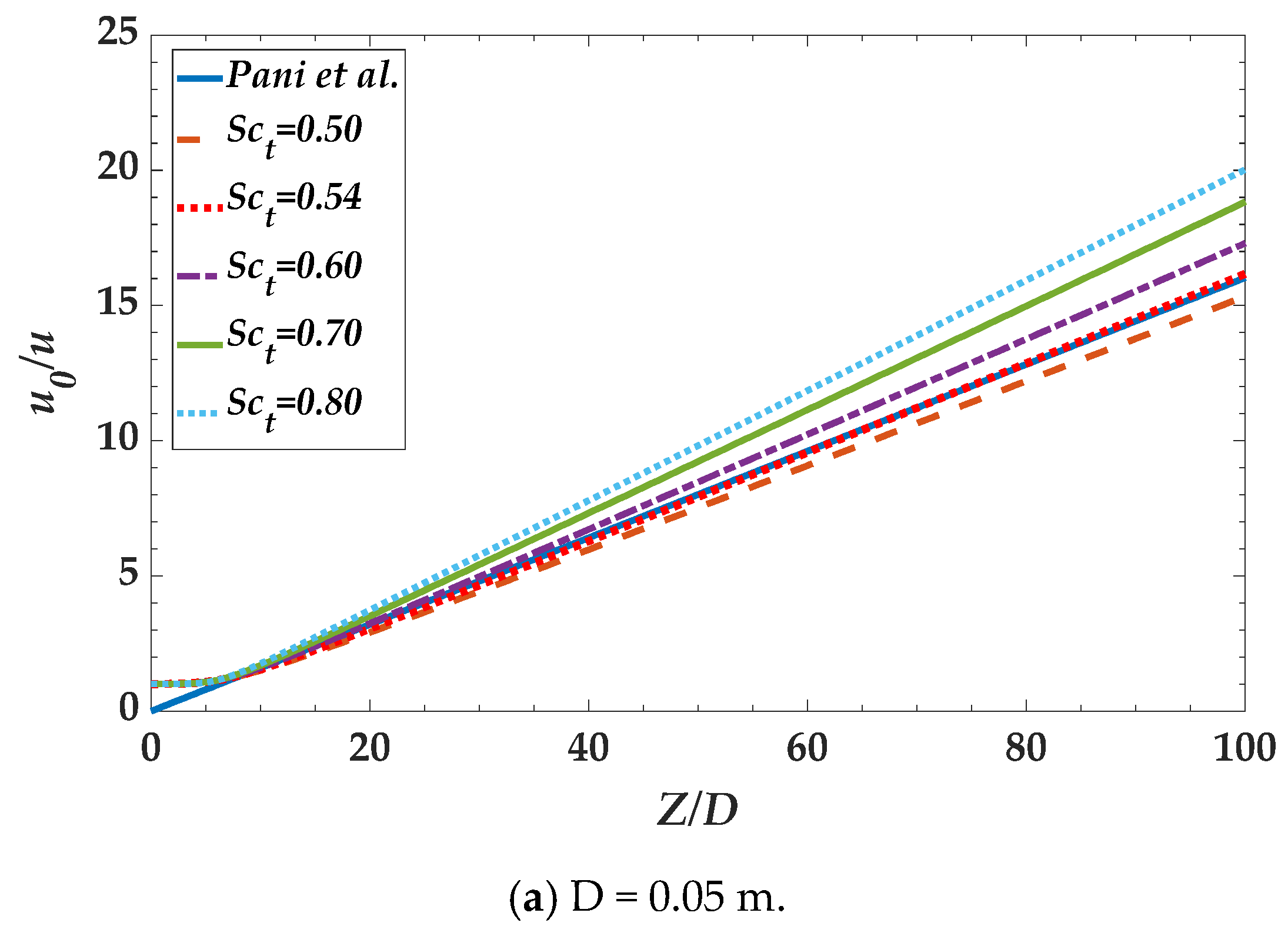
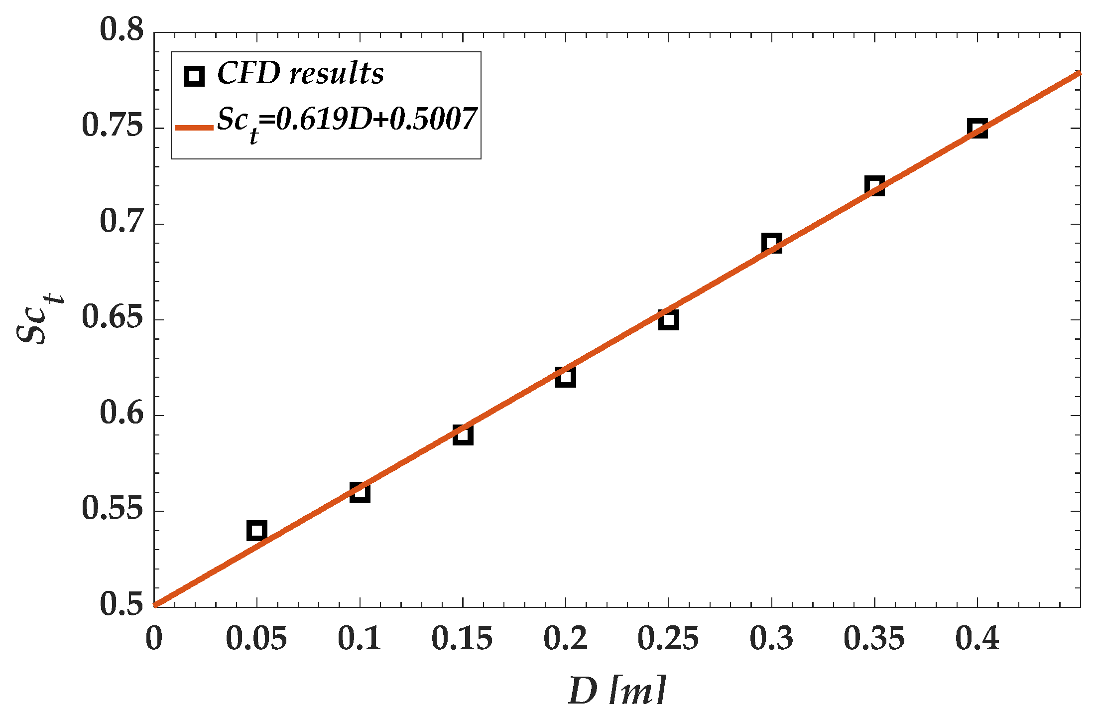
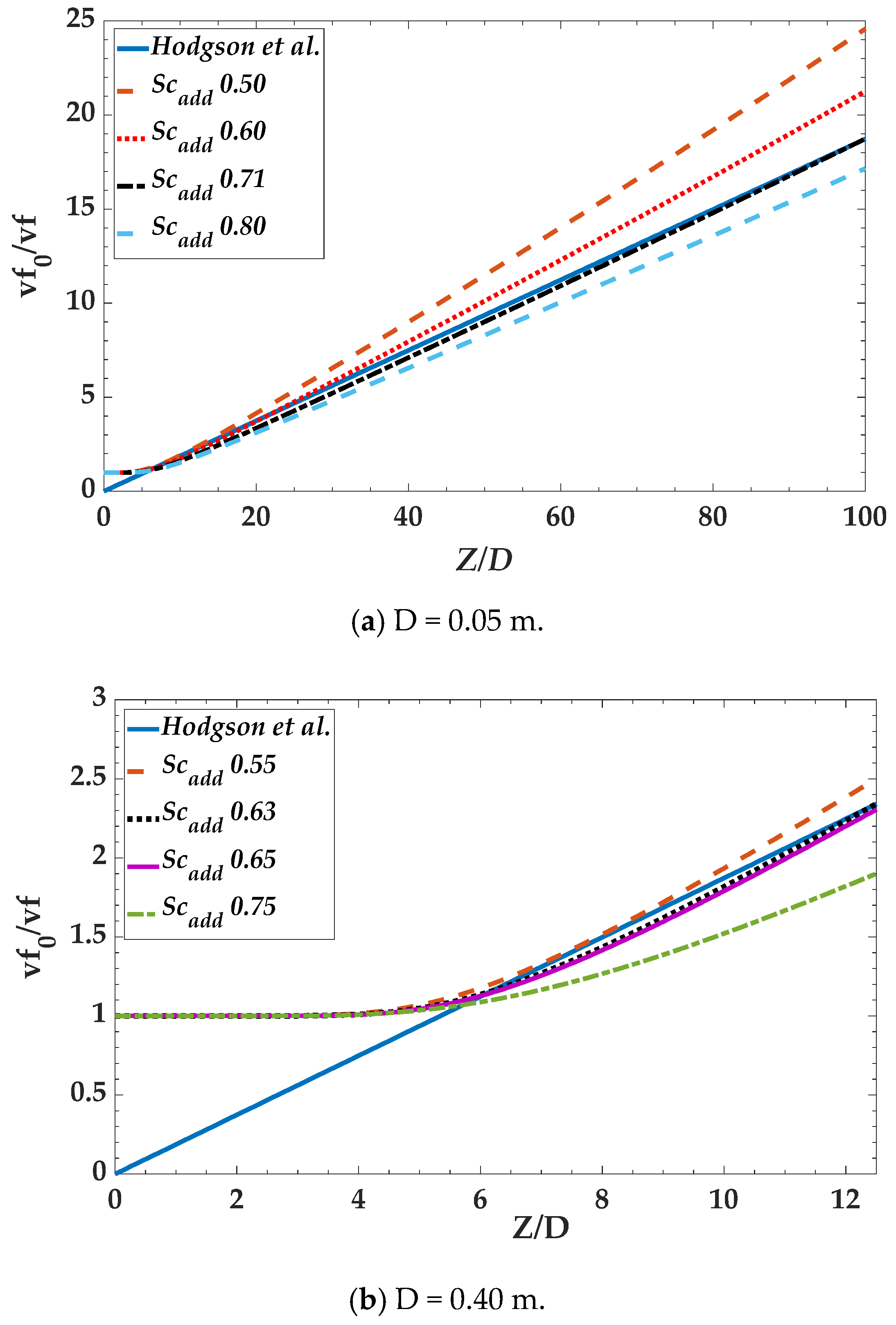
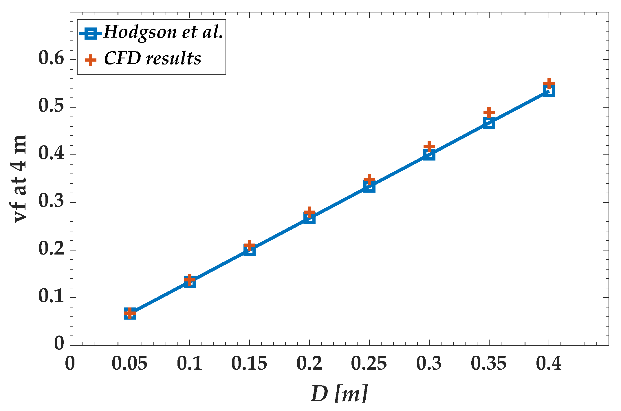
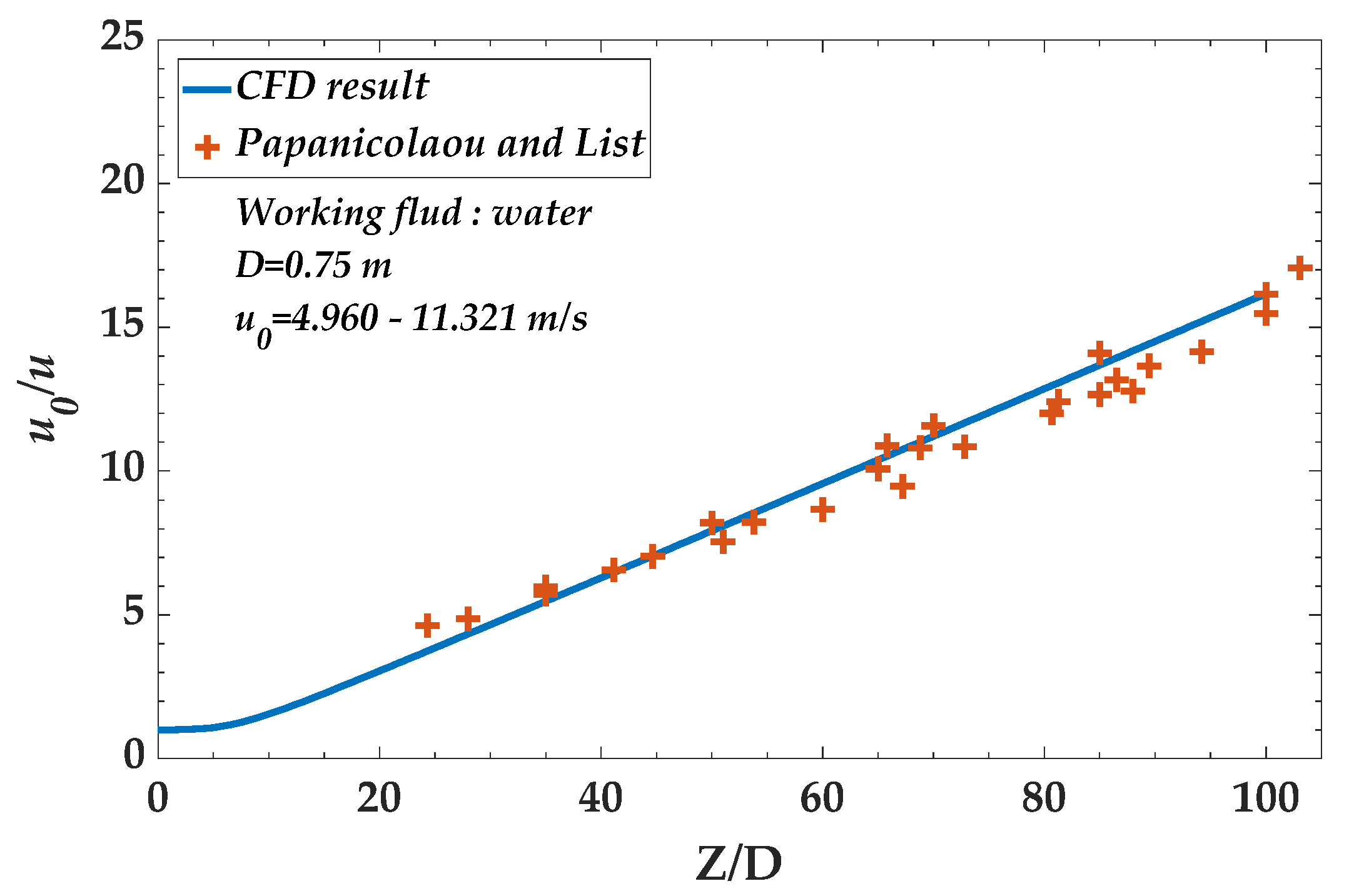
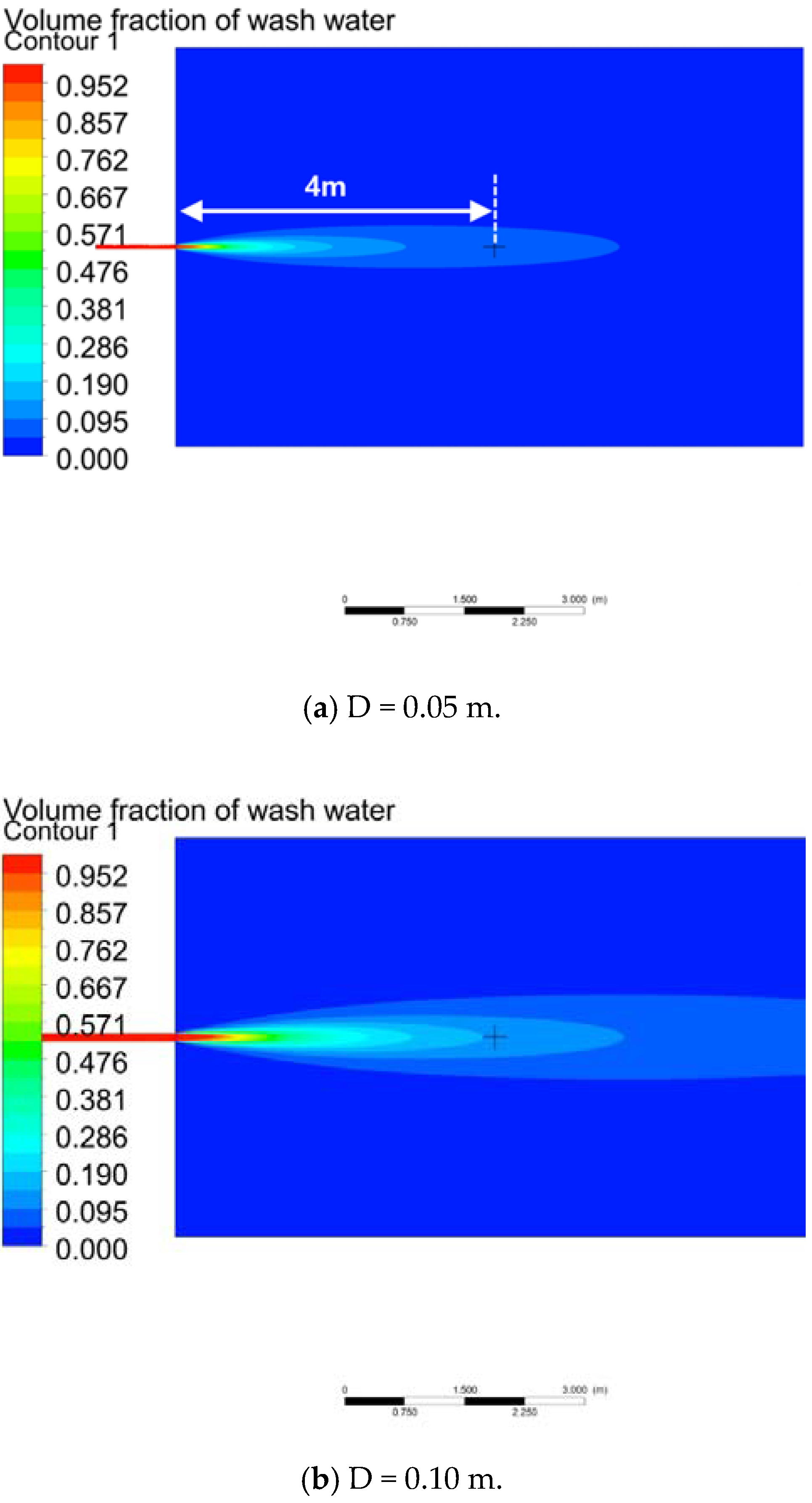
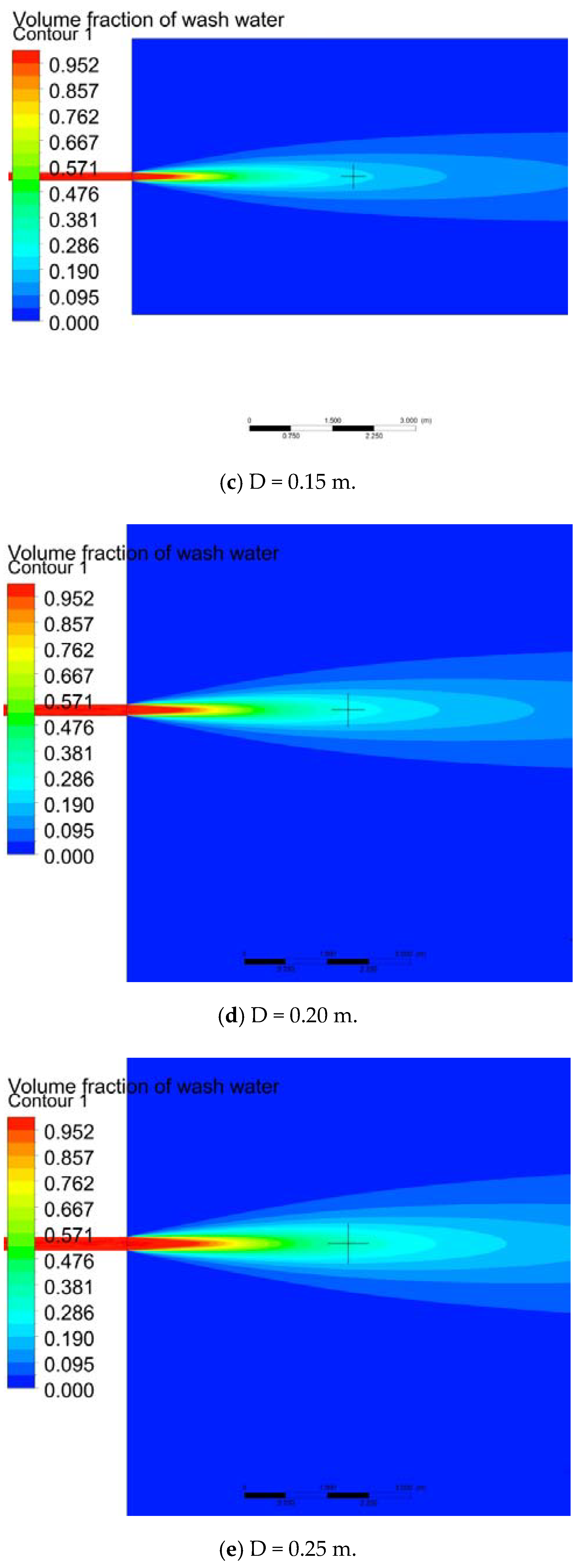
• To simulate the dispersion phenomenon in turbulent jet flow, we solved the transport equation by applying the volume fraction. Simulation was performed for nozzle diameters ranging from 0.05 m to 0.40 m. The turbulent Schmidt number is a critical parameter that exerts a significant effect on dispersion. An appropriate turbulent Schmidt number must be selected according to the nozzle diameter. The appropriate turbulent Schmidt numbers of the transport equations were calculated by comparing them with the existing correlations. The simulation results obtained within 5 m from the discharge point by using the calculated turbulent Schmidt numbers matched well with the results obtained by Pani et al. [14] and Hodgson et al. [20].
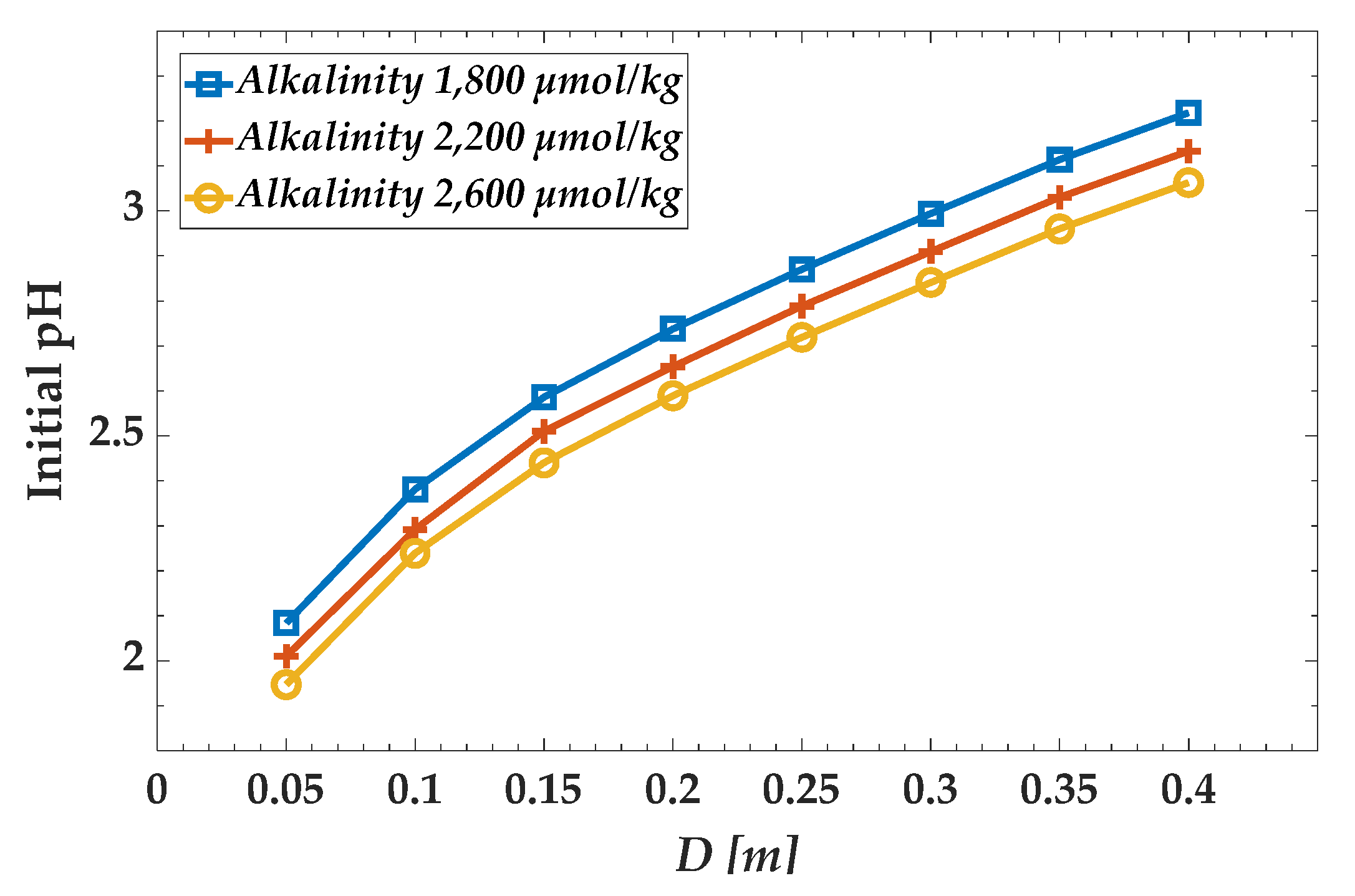
• The volume fraction at 4 m from the discharge point was calculated through simulation, and titration curves were obtained by the theoretical chemical reaction model. The pH value at 4 m can be derived from the initial pH by applying the calculated volume fraction or dilution ratio to the titration curves.
• When the wash water has a low pH, a small diameter nozzle is required to restore the pH to 6.5 at 4 m from the discharge point. When the seawater in the surrounding sea area has a low alkalinity, a large amount of seawater is required. Hence, a small diameter nozzle must be used to promote dispersion. At the initial pH of 3.0 and alkalinity of 2200 μmol/kg, the nozzle diameter should be less than 0.34 m, and at the initial pH of 3.0 and alkalinity of 1800 μmol/kg, it should be less than 0.30 m.
• For future research, we will improve the accuracy of the chemical reaction model through titration experiments by using wash water and seawater obtained from the scrubber of actual ship engines. Moreover, we intend to improve the reliability of the CFD simulation through comparison with correlations derived from more varied turbulent jet flows.

References

1. IMO MEPC 70/18/Add.1 ANNEX6. Effective Date of Implementation of the Fuel Oil Standard in Regulation 14.1.3 of MARPOL ANNEX VI 2016. Available online: http://www.imo.org (accessed on 9 April 2020).
2. Van, T.C.; Ramirez, J.; Rainey, T.; Ristovski, Z.; Brown, R.J. Global impacts of recent IMO regulations on marine fuel oil refining processes and ship emissions. Transp. Res. Part D Transp. Environ. 2019, 70, 123–134. [Google Scholar] [CrossRef]
3. Cheenkachorn, K.; Poompipatpong, C.; Gyeung, C. Performance and emissions of a heavy-duty diesel engine fuelled with diesel and LNG (liquid natural gas). Energy 2013, 53, 52–57. [Google Scholar] [CrossRef]
4. Armellini, A.; Daniotti, S.; Pinamonti, P.; Reini, M. Evaluation of gas turbines as alternative energy production systems for a large cruise ship to meet new maritime regulations. Appl. Energy 2018, 211, 306–317. [Google Scholar] [CrossRef] [Green Version]
5. Tang, X.; Li, T.; Yu, H.; Zhu, Y. Prediction model for desulphurization efficiency of onboard magnesium-base seawater scrubber. Ocean Eng. 2016, 76, 98–104. [Google Scholar] [CrossRef]
6. Ammar, N.R.; Seddiek, I.S. Eco-environmental analysis of ship emission control methods: Case study RO-RO cargo vessel. Ocean Eng. 2017, 137, 166–173. [Google Scholar] [CrossRef]
7. Koski, M.; Stedmon, C.; Trapp, S. Ecological effects of scrubber water discharge on coastal plankton: Potential synergistic effects of contaminants reduce survival and feeding of the copepod Acartia tonsa. Mar. Environ. Res. 2017, 129, 374–385. [Google Scholar] [CrossRef] [PubMed] [Green Version]
8. Ytreberg, E.; Hassellöv, I.M.; Nylund, A.T.; Hedblom, M.; Al-Handal, A.Y.; Wulff, A. Effects of scrubber washwater discharge on microplankton in the Baltic Sea. Mar. Pollut. Bull. 2019, 145, 316–324. [Google Scholar] [CrossRef] [PubMed]
9. Ülpre, H.; Eames, I.; Greig, A. Turbulent acidic jets and plumes injected into an alkaline environment. J. Fluid Mech. 2013, 734, 253–274. [Google Scholar] [CrossRef] [Green Version]
10. Ülpre, H.; Eames, I. Environmental policy constraints for acidic exhaust gas scrubber discharges from ships. Mar. Pollut. Bull. 2014, 88, 292–301. [Google Scholar] [CrossRef]
11. Lipari, G.; Stansby, P.K. Review of experimental data on incompressible turbulent round jets. Flow Turbul. Combust. 2011, 87, 79–114. [Google Scholar] [CrossRef]
12. Panchapakesan, N.R.; Lumley, J.L. Turbulence Measurements in Axisymmetric Jets of Air and Helium. Part 2. Helium Jet. J. Fluid Mech. 1993, 246, 225–247. [Google Scholar] [CrossRef]
13. Boersma, B.J.; Brethouwer, G.; Nieuwstadt, F.T.M. A numerical investigation on the effect of the inflow conditions on the self-similar region of a round jet. Phys. Fluids 1998, 10, 899–909. [Google Scholar] [CrossRef]
14. Pani, B.S.; Lai, A.C.H.; Wong, C.K.C. Turbulent Jets: Point-Source and CFD Simulation Results. J. Environ. Res. Dev. 2011, 5, 952–959. [Google Scholar]
15. Robinson, D.; Wood, M.; Piggott, M.; Gorman, G. CFD modelling of marine discharge mixing and dispersion. J. Appl. Water Eng. Res. 2016, 4, 152–162. [Google Scholar] [CrossRef] [Green Version]
16. Choi, Y.S.; Cha, M.H.; Kim, M.; Lim, T.W. Design of nozzle diameter based on the IMO regulation for discharging scrubber wash-water. J. Korean Soc. Mar. Eng. 2019, 43, 285–291. [Google Scholar] [CrossRef]
17. Ülpre, H. Turbulence Acidic Discharges into Seawater. Ph.D. Thesis, University College London, London, UK, 2015. [Google Scholar]
18. Frankignoulle, M. A complete set of buffer factors for acid / base CO2 system in seawater. J. Mar. Syst. 1994, 5, 111–118. [Google Scholar] [CrossRef]
19. Brown, T.E.; Lemay, H.E.; Bursten, B.E.; Murphy, C.; Woodward, P.; Stoltzfus, M.E. Chemistry: The Central Science, 13th ed.; Pearson: London, UK, 2014. [Google Scholar]
20. Hodgson, J.E.; Moawad, A.K.; Rajaratnam, N. Concentration field of multiple circular turbulent jets. J. Hydraul. Res. 1999, 37, 249–256. [Google Scholar] [CrossRef]
21. Eigen, M. Methods for investigation of ionic reactions in aqueous solutions with half-times as short as 10–9 sec Application to neutralization and hydrolysis reactions. Discuss. Faraday Soc. 1954, 17, 194–205. [Google Scholar] [CrossRef]
22. Oliver, C.J.; Davidson, M.J.; Nokes, R.I. k-ε Predictions of the initial mixing of desalination discharges. Environ. Fluid Mech. 2008, 8, 617–625. [Google Scholar] [CrossRef]
23. Shirzadi, M.; Mirzaei, P.A.; Naghashzadegan, M. Aerodynamics Improvement of k-epsilon turbulence model for CFD simulation of atmospheric boundary layer around a high-rise building using stochastic optimization and Monte Carlo Sampling technique. J. Wind Eng. Ind. Aerodyn. 2017, 171, 366–379. [Google Scholar] [CrossRef]
24. ANSYS CFX-Theory Guide; V13.0.; Ansys Inc.: Canonsburg, PA, USA, 2010.
25. He, G.; Guo, Y.; Hsu, A.T. The Effect of Schmidt Number on Turbulent Scalar Mixing in a Jet-in-Crossflow. Int. J. Heat Mass Transf. 1999, 42, 3727–3738. [Google Scholar] [CrossRef]
26. Nguyen, V.T.; Nguyen, T.C.; Nguyen, J. Numerical Simulation of Turbulent Flow and Pollutant Dispersion in Urban Street Canyons. Atmosphere 2019, 10, 683. [Google Scholar] [CrossRef] [Green Version]
27. Papanicolaou, P.N.; List, E.J. Investigations of Round Vertical Turbulent Buoyant Jets. J. Flud Mech. 1988, 195, 341–931. [Google Scholar] [CrossRef]
Figure 1. Mesh independence on the number of nodes.
Jmse 08 00272 g001
Figure 2. Hexahedral mesh for CFD simulations.
Jmse 08 00272 g002
Figure 3. Titration curves obtained by the theoretical chemical reaction model.
Jmse 08 00272 g003
Figure 4. Relationship between dimensionless velocity ( u 0 / u ) and dimensionless distance ( Z / D ) under different turbulent Schmidt numbers.
Jmse 08 00272 g004aJmse 08 00272 g004b
Figure 5. Relationship between valid turbulent Schmidt number and the nozzle diameter.
Jmse 08 00272 g005
Figure 6. Relationship between volume fraction ratio ( v f 0 / v f ) and dimensionless distance ( Z / D ) under different turbulent Schmidt numbers of additional variable.
Jmse 08 00272 g006
Figure 7. Relationship between valid turbulent Schmidt number and nozzle diameter of additional variable.
Jmse 08 00272 g007
Figure 8. Comparison between existing correlation and CFD results.
Jmse 08 00272 g008
Figure 9. Comparison between the CFD results and the experimental data* (* reproduced from the work of Papanicolaou and List (1988) [27]).
Jmse 08 00272 g009
Figure 10. Variation in the treatable initial pH with the designed nozzle diameter under different seawater alkalinity values.
Jmse 08 00272 g010