Article

Numerical Simulation on Vortex Shedding from a Hydrofoil in Steady Flow

College of Shipbuilding Engineering, Harbin Engineering University, Harbin 150001, China
*
Author to whom correspondence should be addressed.
J. Mar. Sci. Eng. 2020, 8(3), 195; https://doi.org/10.3390/jmse8030195
Submission received: 19 February 2020 / Revised: 2 March 2020 / Accepted: 3 March 2020 / Published: 12 March 2020
(This article belongs to the Section Ocean Engineering)

Abstract

:
This paper presents a numerical modeling procedure for the idealization of vortex shedding effects in the wake flow field of a NACA0009 hydrofoil. During the simulation, the lift and drag acting on the hydrofoil were monitored, and the vortex-shedding frequency of the hydrofoil was analyzed. The effects of inflow velocity, trailing-edge thickness, angle of attack, and maximum hydrofoil thickness on vortex shedding were investigated. The results indicate that an increase in the inflow velocity led to an increase in the vortex-shedding frequency and a negligible change in the Strouhal number. Furthermore, as the thickness of the trailing edge increased, the vortex-shedding frequency decreased gradually, whereas the Strouhal number first increased and then decreased. Vortex shedding and lift curve oscillations ceased altogether after the angle of attack of the hydrofoil increased beyond a certain threshold. When the maximum hydrofoil thickness was increased while keeping the thickness and chord length of the trailing edge constant, the vortex-shedding frequency decreased.

1. Introduction

Vortex shedding from the trailing edge of a foil is a significant phenomenon in various engineering disciplines. Flows separated by a foil will recombine at the upper and lower surfaces of the trailing edge of the foil, forming periodic eddies in the wake field and inducing mechanical vibrations. This phenomenon was first observed in aircraft airfoils; because airfoils typically exhibit very high wake-vortex shedding frequencies, they are at a considerable risk of fatigue damage. The damage caused by vortex shedding is particularly severe if the vortex-shedding frequency approaches a natural frequency of the airfoil. A similar phenomenon is known to occur in propellers and is particularly concerning in marine propellers because an intense degree of vortex shedding leads to periodic fatigue stresses in the blades of the propeller that shorten their service life. Because vortex shedding can lead to a series of failures in engineered structures, it is important to study the causes of this phenomenon and elucidate the behavior of vortex shedding in a variety of operating conditions.
The mechanical vibrations induced by vortex shedding have been widely investigated. Vincenc Strouhal discovered that the audible tone of a wire “singing” in the wind is proportional to the quotient of the wind speed by the wire thickness (i.e., tone = proportionality coefficient × wind speed/wire thickness) and that each cross-section has a certain proportionality coefficient in the noncritical range of Reynolds numbers. This is known as the Strouhal number, and it is an important parameter to evaluate the vortex-shedding frequency. Theodore von Kármán linked this phenomenon to the stable and staggered vortices that form behind a cylindrical object, which was later termed the Kármán vortex street effect. In addition, he proposed the theory of vortex street stability [1]. Perry et al. [2] obtained images of the vortex-shedding process from the wake field of a circular cylinder by tracing the motion of aluminum particles in long-exposure photography. Griffin [3] and Williamson et al. [4] investigated the alternating shedding of vortices from a cylinder and discovered that this process is caused by interactions between vortices on the upper and lower surfaces of the cylinder; once a vortex on a given surface reaches a sufficient strength, it draws the opposing shear layer across the near wake, causing the vortices to shed alternatingly from the upper and lower surfaces. Gerrard [5] observed vortex shedding from circular and bluff cylinders with different cross-sectional shapes and deduced that the vortex generation is affected by the end conditions of the cylinders. Gerich [6] proved that the shape of the ends of a cylinder affect the mechanism of vortex shedding from these ends. In addition, Achenbach and Heinecke [
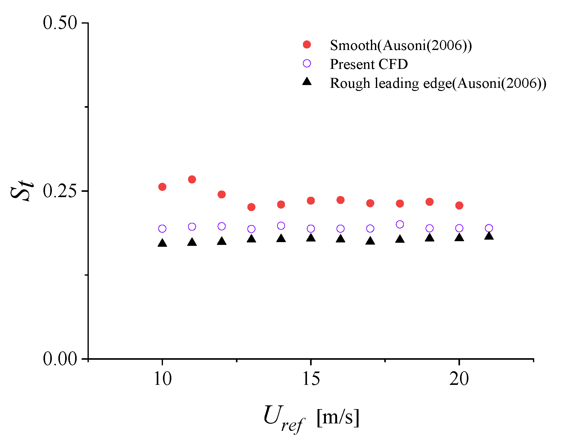
7] conducted wind tunnel experiments and discovered that the wake of a cylinder became more regular as the roughness of the cylinder’s surface increased. Furthermore, the Strouhal number of a vortex shedding from a rough cylinder was estimated to be much smaller than that of a vortex shedding from a smooth cylinder.
Through the various studies conducted on the vortex-shedding phenomenon, it was observed that intense resonance can occur if the vortex-shedding frequency of the Kármán vortex street is equal to one of the eigenfrequencies of a given object. This discovery shifted the focus of the study of vortex shedding from simple cylindrical objects to objects of practical interest, such as hydrofoils. A series of analytical studies were also conducted on the basis of experimental data. Ausoni [8] experimentally investigated the effects of cavitation on vortex shedding from symmetrical hydrofoils with a blunted trailing edge and analyzed the wake structure, vortex-shedding frequency, and hydrofoil resonance frequency associated with each stage of cavitation development. He discovered that the vortex-shedding frequency can “lock-in” to an eigenfrequency of a hydrofoil. Lotfy and Rockwell [9] investigated vortex shedding in the near-wake of an oscillating trailing edge. Prasad and Williamson [10] analyzed the vortex dynamics of hydrofoil wakes based on the instability of the shear layer separating the water from a bluff body. Dwayne et al. [11] investigated vortex shedding at a high Reynolds number from hydrofoils with different terminating bevel angles on their trailing edges and found that the vortex-shedding intensity is higher in blunter and thicker trailing edges. Zobeiri et al. [12] conducted an experimental study on the effects of the trailing-edge shape on vortex shedding and flow-induced vibrations and found that oblique trailing edges significantly reduce flow-induced vibrations. This was attributed to the collisions between upper and lower vortices in an oblique trailing edge, which leads to vorticity redistribution.
Numerical modeling has been widely employed for the study of vortex shedding. Many previous numerical studies focused on vortex shedding from circular objects. For example, Williamson [13] numerically simulated the wake flows of a cylindrical object. William [14] used complex analysis to formulate an analytical expression for the shedding frequency of Kármán vortex streets from the trailing edge of an airfoil. However, the shedding frequencies predicted by this expression were typically much lower than the experimentally observed ones. Huerre and Monkewitz [15] and Oertel et al. [16] analyzed the effects of flow instabilities on vortex-shedding behaviors of blunt hydrofoils analytically. Potential flow theory is often used to study the wake-vortex shedding of swinging or flapping objects. However, current studies on vortex shedding focus on the formation of Kármán vortex streets behind static objects, which is essentially a boundary layer dissociation problem; these problems are very difficult to model with the potential flow theory. Another significant feature of this problem is that the trailing edge of the hydrofoil is often very thin, which leads to very large local Reynolds numbers. This results in unique physical phenomena that can only be modeled by precise numerical simulations. Lee et al. [17] studied the vortex shedding of hydrofoils, numerically considering a variety of trailing-edge shapes, and compared their findings with the experimental findings of Ausoni and Zobeiri. In addition, they investigated the effects of periodically varying free-stream flows on vortex shedding.
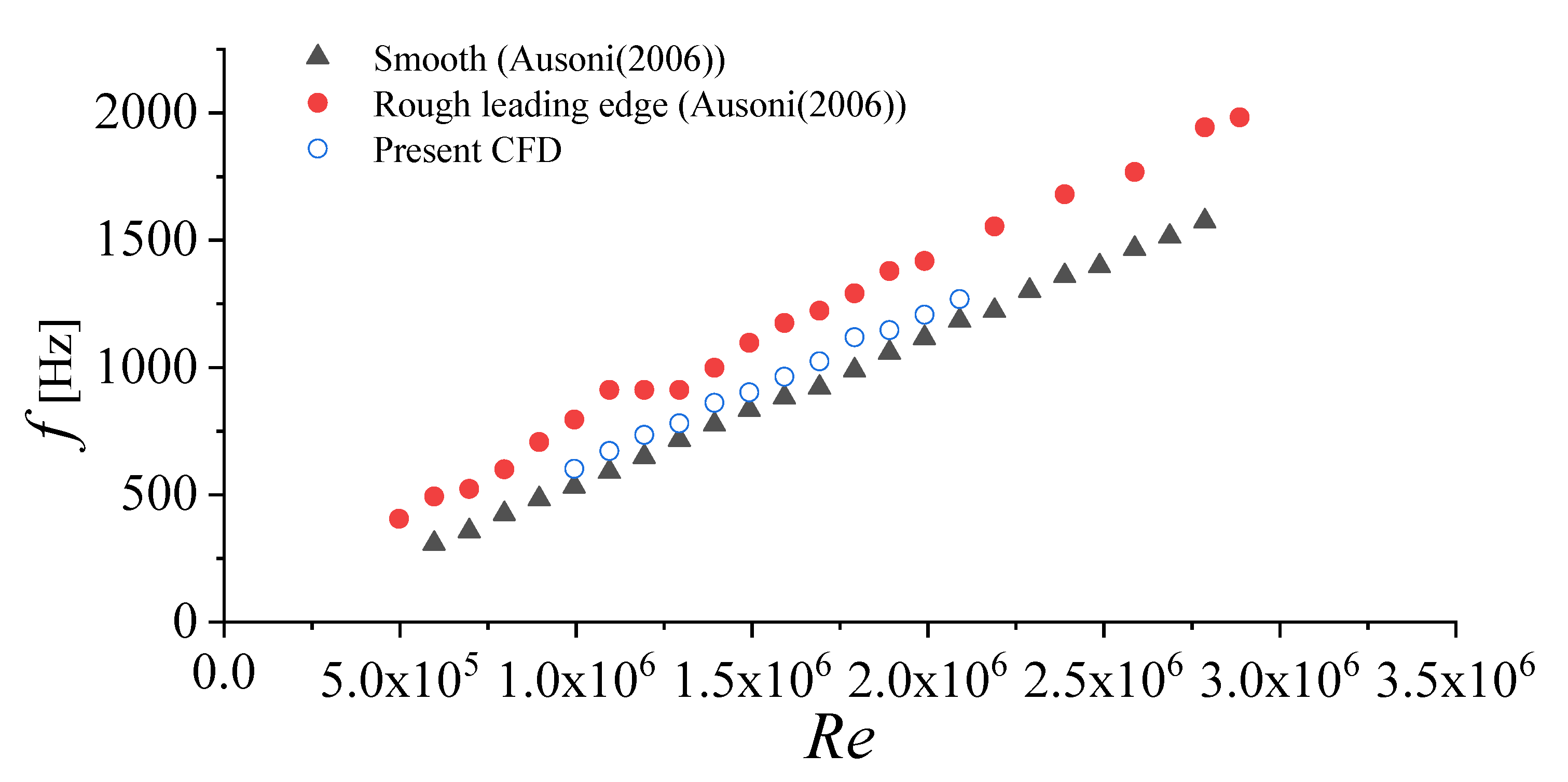
Many studies using numerical simulations of or experimental tests on vortex shedding have been conducted, and the subsequent hydrodynamic force fluctuations of hydrofoils have been analyzed. The main purpose of the abovementioned studies was to evaluate the amplitude and frequency of force fluctuation, which have significant effects on marine structures. Ausoni [8] experimentally studied the vortex-shedding frequency of hydrofoils with perpendicularly truncated trailing edges and found that the increase in frequency was almost linear with the inflow velocity. Dwayne et al. [11] studied the vortex-shedding frequency of hydrofoils with obliquely truncated trailing edges and found that thicker hydrofoils or blunter trailing edges correspond to higher vortex-shedding frequencies. Another experimental study was conducted by Zobeiri [12], wherein it was found that the obliquely truncated trailing edges can significantly reduce the vortex-shedding strength, and subsequently, the amplitude of the force fluctuation. Analytical studies of vortex shedding were performed by Blake [14] and Oertel [16] on hydrofoils and cylinders, respectively. However, the force of analytical results is much less than that by experiments. The vortex shedding of hydrofoils is strongly related to the formation of viscous boundary layers. From this perspective, methods based on the potential flow assumptions can hardly predict vortex shedding precisely. Instead, computational fluid dynamics (CFD) simulations can effectively represent vortex shedding. Although Reynolds-averaged Navier–Stokes simulations [8] or large Eddy simulations (LES) [17] cannot fully simulate turbulent flows, their numerical results generally agree well with experimental results and can reflect the physical characteristics of vortex shedding.
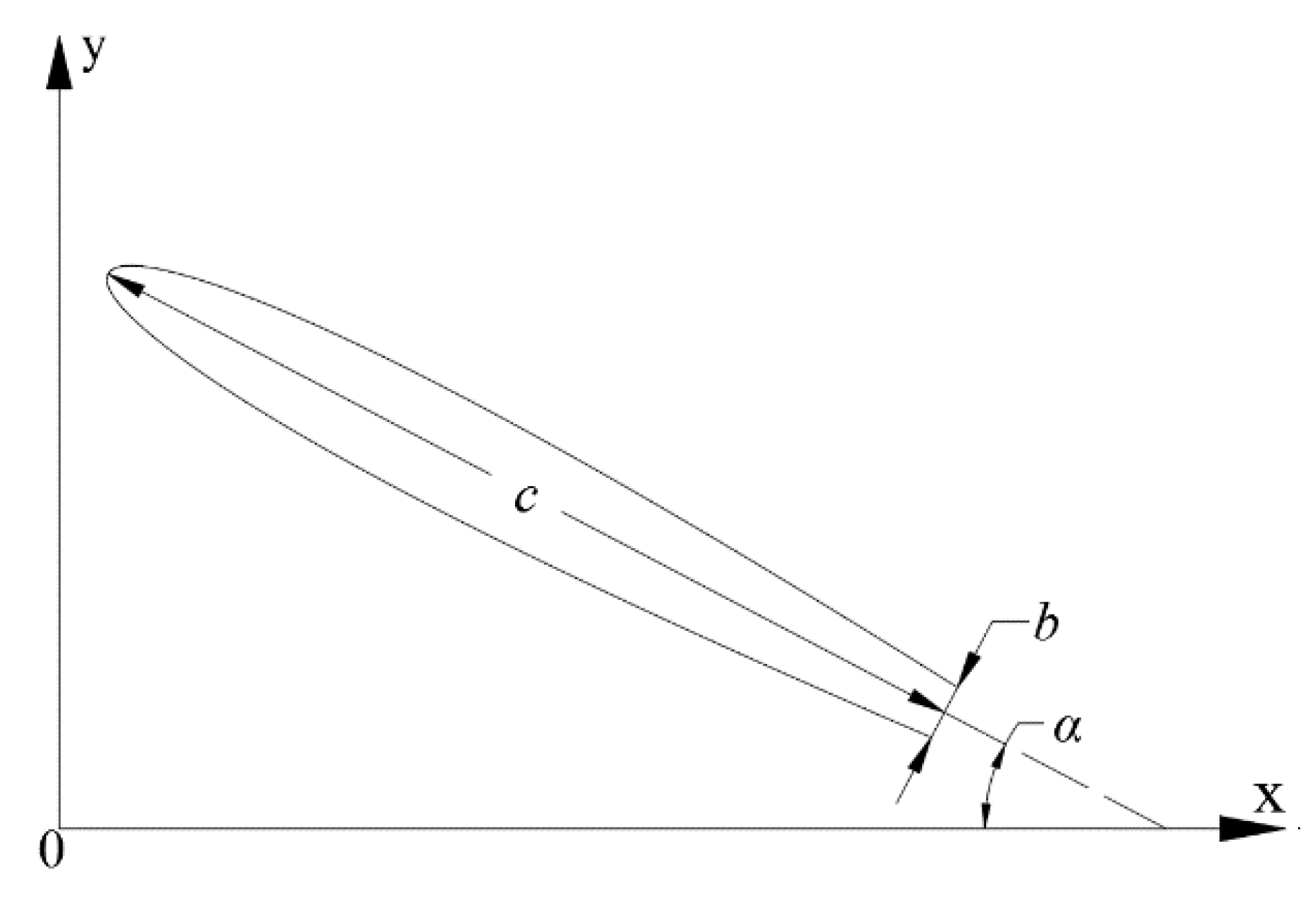
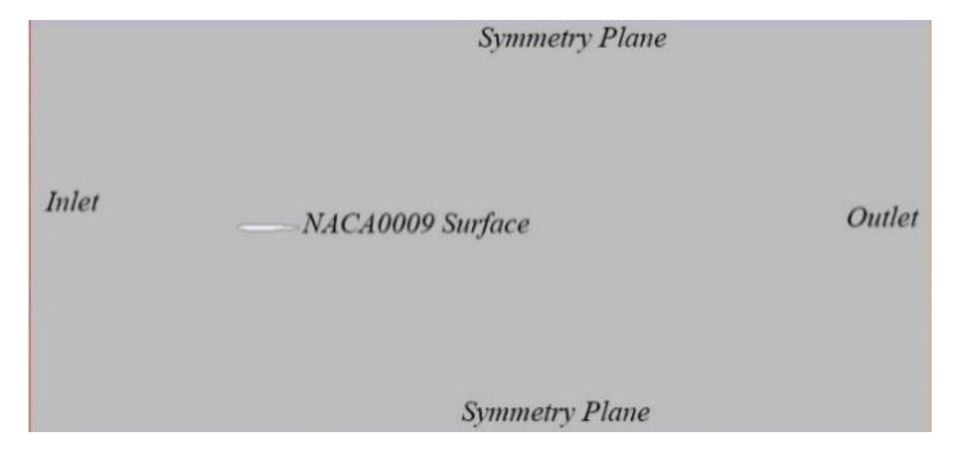
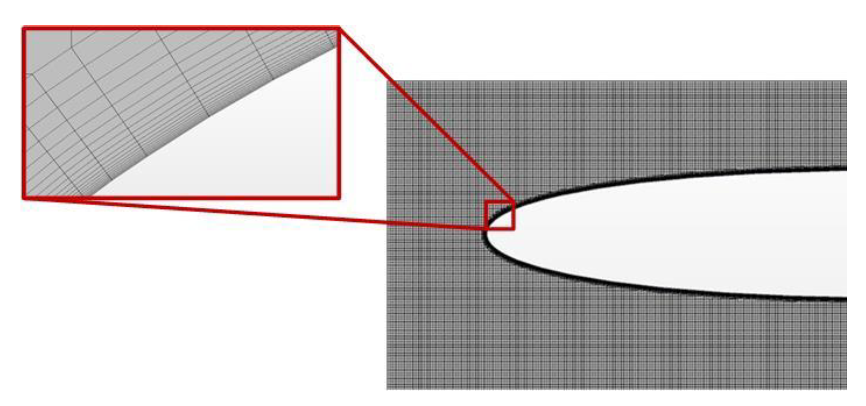
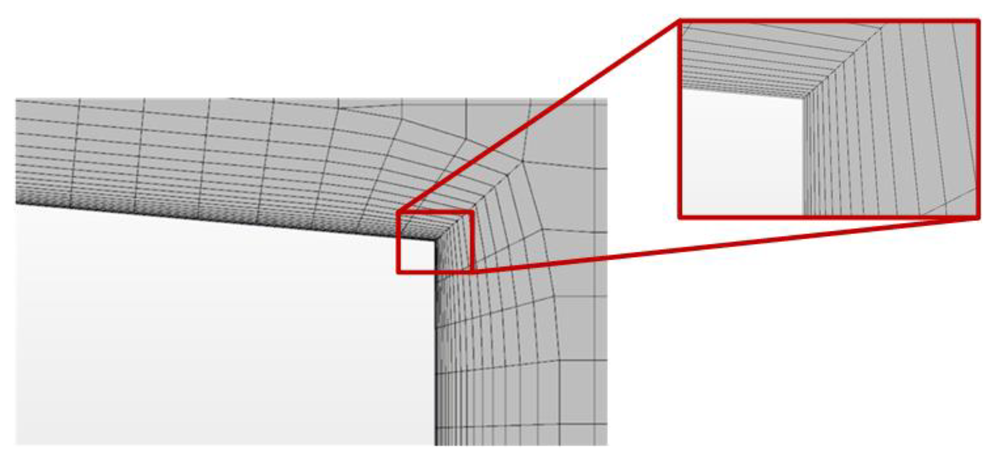
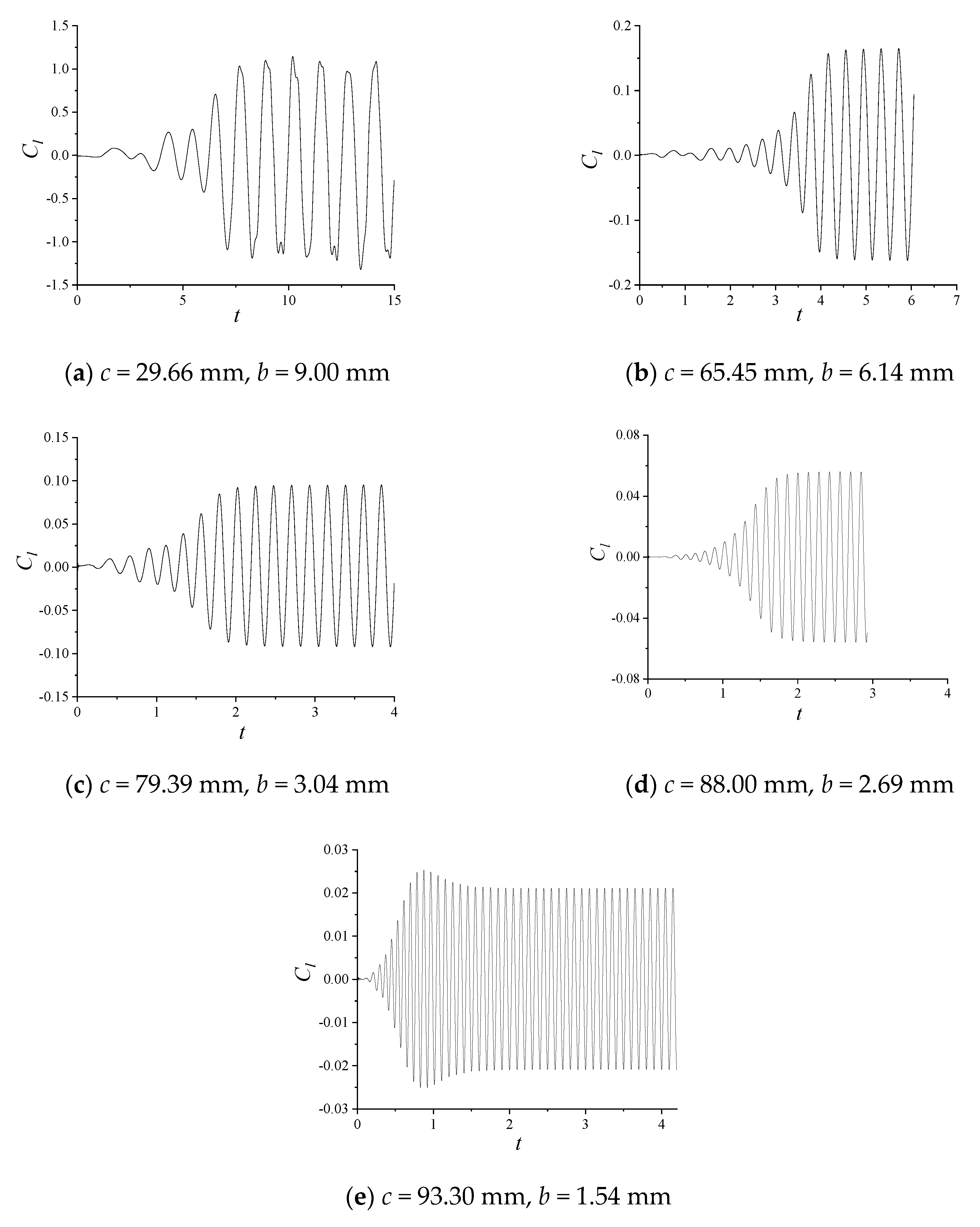
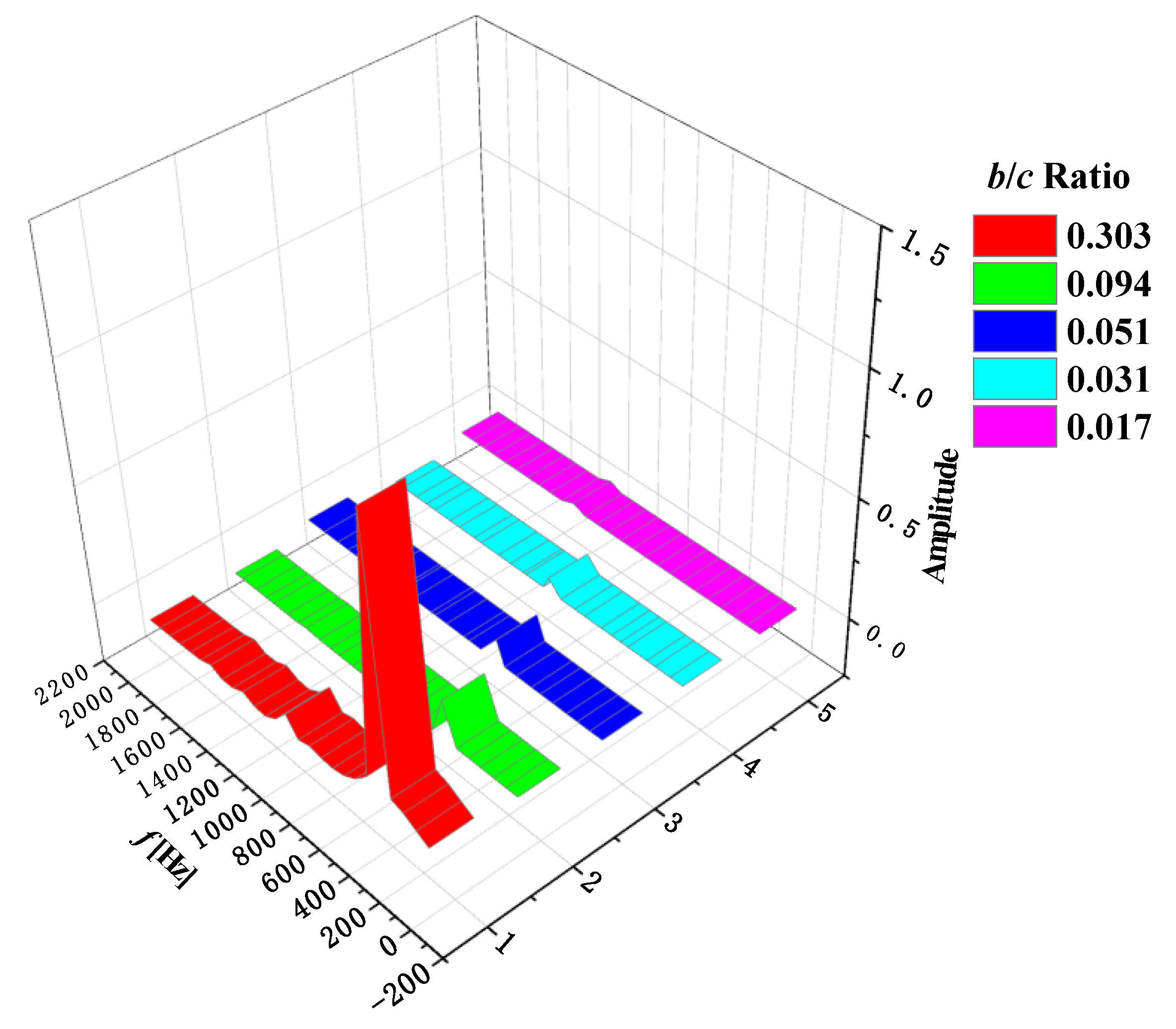
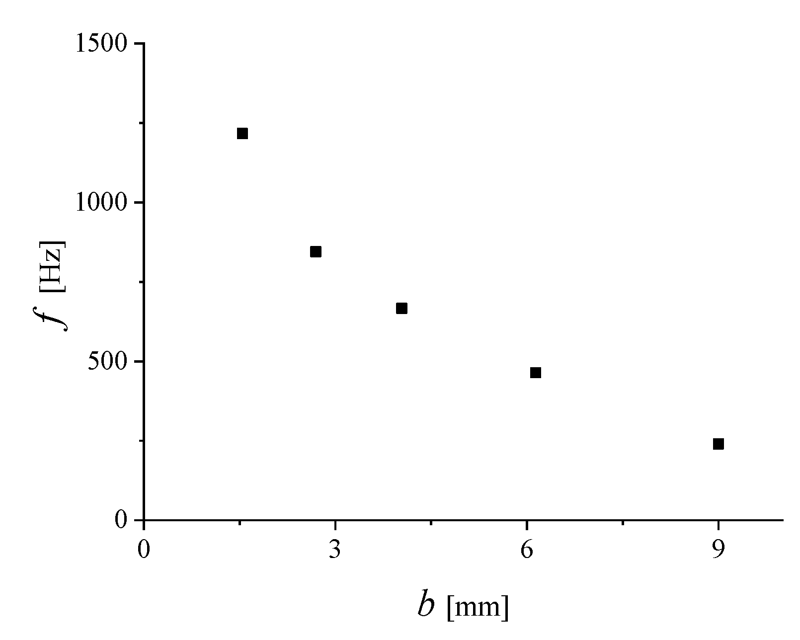
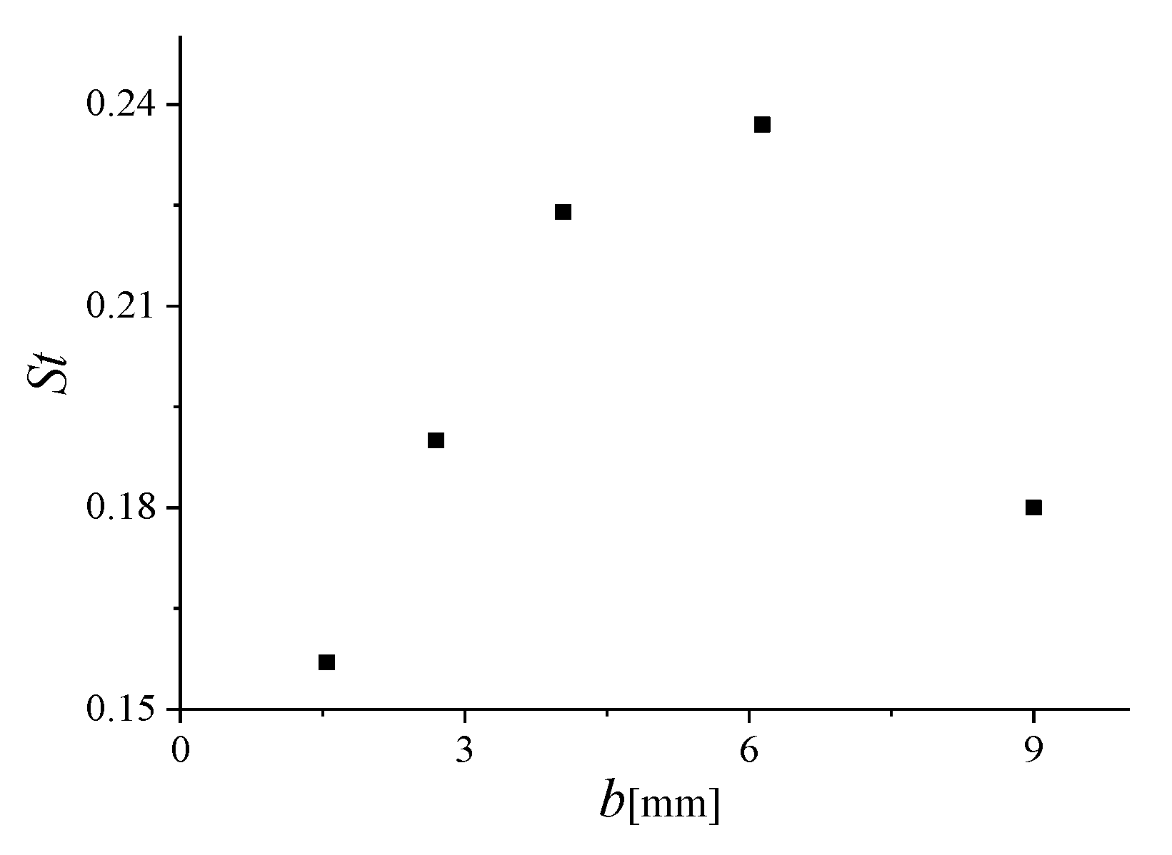
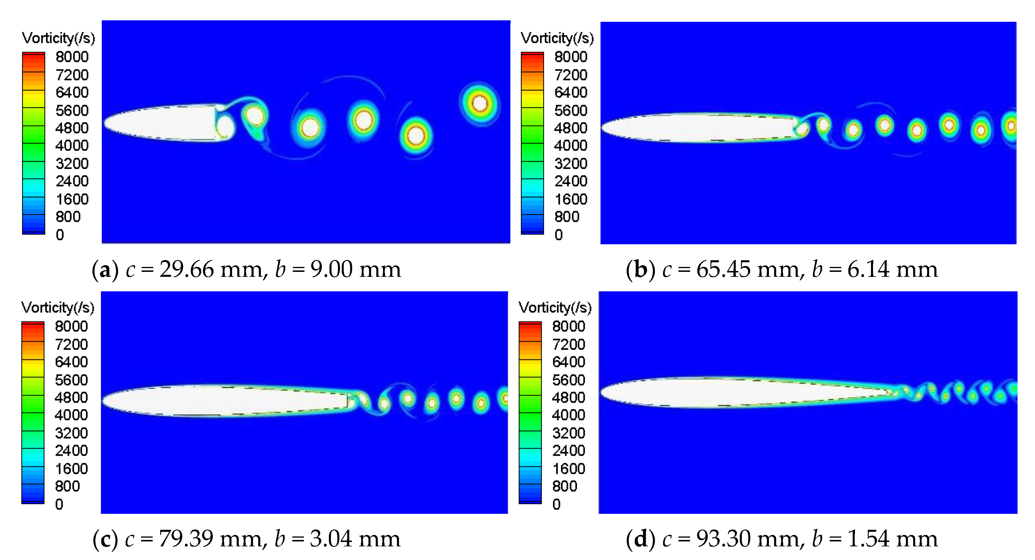
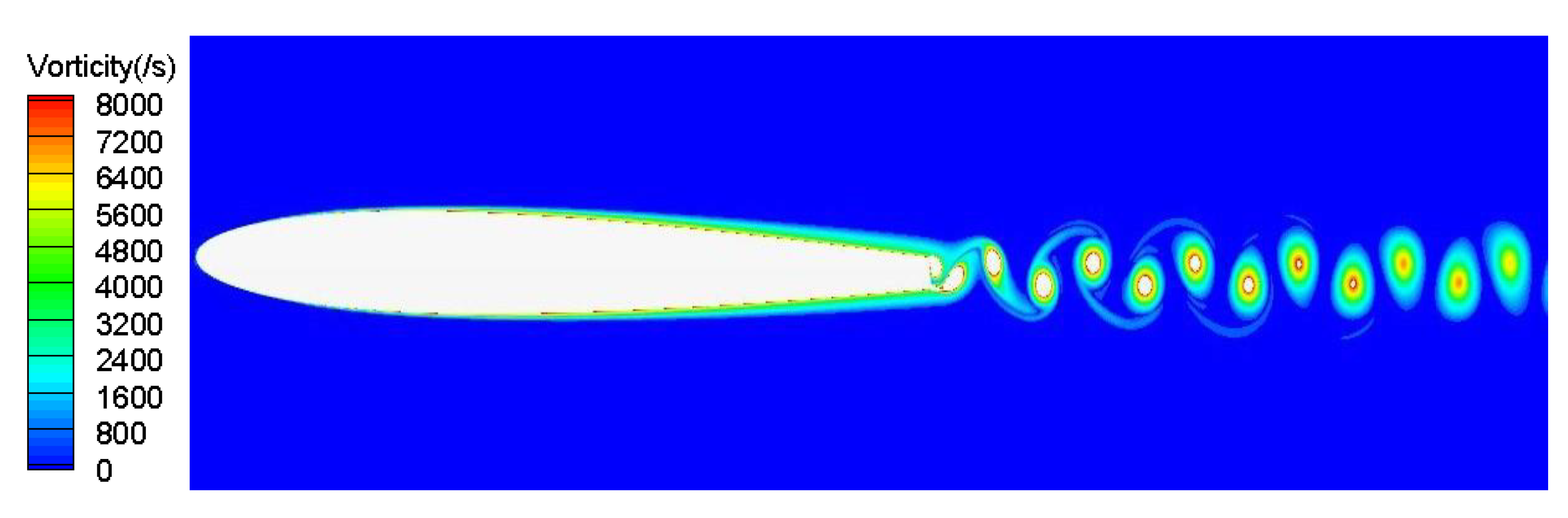
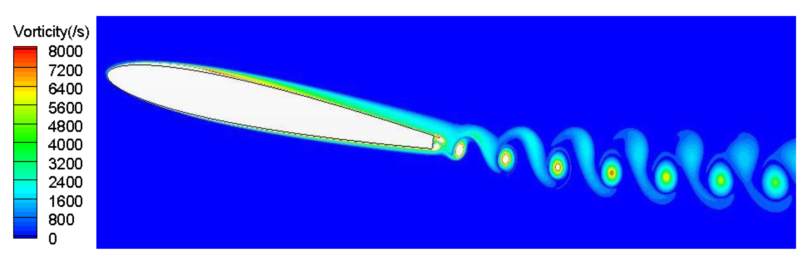
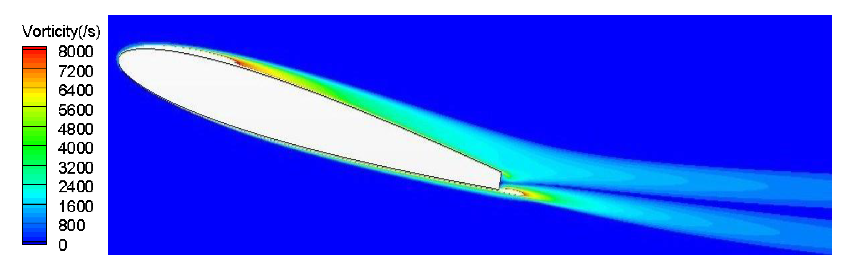
The above discussion shows that vortex shedding from static hydrofoils is a problem of practical significance and academic interest as it plays a significant role in flow-induced vibrations and noise and fatigue damage. However, research on this problem is still insufficient, and further elucidations are required. In this study, we conducted CFD simulations of two-dimensional flows around a NACA0009 hydrofoil in a variety of operating conditions to observe vortex shedding at the trailing edge of a hydrofoil. We investigated the lift curve and trailing-edge vortex shedding of the hydrofoil with different inflow velocities, angles of attack, truncation points, and maximum hydrofoil thicknesses to reveal their correlations with the vortex-shedding frequency. The findings of this study will provide general rules for the investigation of flow-induced vibrations in objects such as hydrofoils and marine propellers.

2. Materials and Methods

2.1. Mathematical Modeling

In this study, the finite volume method, which satisfies the conservations of mass and momentum, was used to solve the integral equations. The vertex-centered method was adopted to form the control elements; the second-order upwind scheme was used for the discrete differentials; the semi-implicit method for pressure linked equations scheme was used for the flow solution. It firstly assumes a velocity distribution u * , v * , Φ * ( u , v , Φ ) in the flow field and then calculates the coefficients and constants in the discrete-form momentum equations at the first iteration. Then, it guesses the pressure p * ; it solves the discrete momentum equation from the pressure field and the pressure correction equation from the velocity field. After correcting the calculated pressure and velocity, all other variables of the control equation are solved. Finally, the results are verified and iterated until convergence.
Numerical simulations were performed using the Spalart–Allmaras (S-A) turbulence model, which is suitable for high-precision boundary-layer computations, e.g., lift computations.
Spalart and Allmaras [18] argued that energy and information flow from large scales to smaller scales in free shear flows and represented the turbulent eddy viscosity coefficient by two terms: a production term and a diffusion term. They constructed a one-equation turbulence model by utilizing the experience gained from other turbulence models and by amending the other turbulent flow-field models.
In the S-A equation, the definition of Reynold stress is:
u i u j ¯ = 2 v t S i j , S i j ( U i / x j + U j / x i ) / 2
where, the turbulent eddy viscosity vt can be expressed as:
v t = v ˜ f v 1 , f v 1 = χ 3 χ 3 + c v 1 3 , χ v ˜ v ,
where v is the kinematic molecular viscosity and is the working variable. From the above equations, we obtain the transport equation:
D v ˜ D t = c b 1 [ 1 f t 2 ] S ˜ v ˜ + 1 σ [ ( ( v + v ˜ ) v ˜ ) + c b 2 ( v ˜ ) 2 ] [ c w 1 f w c b 1 κ 2 f t 2 ] [ v ˜ d ] + f t 1 Δ U 2 ,
where S(~) is the magnitude of vorticity; b is the distance to the nearest wall; ΔU is the velocity difference between a point in the fluid and a point on the wall; ft1, ft2, and fw are functional equations, and the rest of the symbols represent constants. The specific definitions of these symbols are as follows:
S ˜ S + v ˜ κ 2 d 2 f v 2 ,   f v 2 = 1 χ 1 + χ f v 1
f t 1 = c t 1 g t exp ( c t 2 w t 2 Δ U 2 [ d 2 + g t 2 d t 2 ] ) , g t min ( 0.1 , Δ U / w t Δ x ) ,
f t 2 = c t 3 exp ( c t 4 χ 2 ) ,
f w = g [ 1 + c w 3 6 g 6 + c w 3 6 ] 1 / 6 ,   g = r + c w 2 ( r 6 r ) ,   r v ˜ S ˜ κ 2 d 2 ,
The S-A turbulence model is more computationally efficient than two-equation turbulence models, and it is also very stable and accurate. The S-A model accurately simulates the region of the wake where strain rates are dominated by vorticity, and it predicts the turbulent eddy viscosity.

2.2. Test Case and Computational Mesh

In this study, a two-dimensional flow method was used to study vortex shedding. The model used in this study was a NACA0009 hydrofoil with a chord length c of 100 mm and a trailing-edge thickness b of 3.22 mm, which is identical to the model used by Ausoni et al. (2006). Figure 1 shows a diagram of the hydrofoil model with the chord length (c), trailing-edge thickness (b), and angle of attack (α).
To avoid the effects of the computational boundaries illustrated in Figure 2 on the flow simulation, the domain was set to relatively large dimensions (13c × 6c). Typically, the outlet boundary has a greater effect than the inlet boundary owing to the downstream vortex shedding. Thus, the hydrofoil was further from the outlet than from the inlet. Neglecting the mutual effect between the inlet boundary and the hydrofoil, the inlet was set as the velocity inlet. To achieve better conservation and more stable simulations, the outlet was set as the pressure outlet rather than the velocity outlet. To further avoid the effects of the boundaries, the upper and lower boundaries were set as symmetrical and slipping, different from the nonslipping surfaces of the hydrofoil.
The grid around the hydrofoil is shown in Figure 3. Two mesh types were used in the computational domain, namely trimmed and prism layer meshes. The trimmed mesh was the primary type of mesh used in the fluid region. This part of the mesh consisted of quadrilateral elements parallel to the inflow; this configuration reduces truncation errors in the calculation. Prism layer meshes were used to generate the boundary layers. A 3c × 2c refined region was set up around the hydrofoil to refine the flows around it, and the mesh size in this region was 5% of that of the unrefined region. The computational domain contained a total of 2,495,989 mesh elements.
Figure 4 shows the boundary layer grid of the hydrofoil. In these computations, physical variables tend to vary most significantly around boundaries. Therefore, a refined boundary layer mesh was used in the calculations. The thickness of the first mesh layer was determined by the Y+ value. Because the Reynolds number in the simulation was quite large (Re = 1,194,257.2), the fluid flow became fully turbulent at positions close to the surface of the hydrofoil. Therefore, the Y+ value was set to 1, which yielded a first mesh layer thickness of 1.97 × 10⁻⁶ m. The growth rate of the prism layer mesh was set to 1.2, and the boundary layer mesh was configured with a total of 20 layers to ensure a smooth transition into the outer mesh. The total thickness of the boundary layer mesh was 3.67 × 10⁻⁴ m.

2.3. Convergence Analysis

2.3.1. Mesh Convergence

Using the meshing strategy reported by Ausoni et al. [8], a refined mesh was configured to assess the mesh convergence.
The medium mesh had a total of 2,495,989 elements, and the thickness of the boundary layer was 3.67 × 10⁻⁴ m. The mesh size was further increased and reduced to verify the mesh convergence, and the resulting mesh had medium and fine grids with 1,562,259 and 4,027,882 elements, respectively. When the grid scale was changed between coarse, medium, and fine while keeping the number of boundary layers constant, the extension rates of the layers changed to 1.4, 1.3, and 1.2, respectively.
Then, the time step was set to 1 × 10⁻⁶ s. Table 1 lists the drag coefficient C d , maximum lift coefficient C l (max), and Strouhal number ( S t ) obtained with different grid scales.
From Table 1, it can be observed that the calculation results with the three grid conditions are similar. The mesh size was further reduced under the medium mesh condition, and the resulting C d , C l , and S t changed by 1.9%, 1.5%, and 2.6%, respectively. The degree of change in data is small, and thus, it can be considered grid-independent.

2.3.2. Time-Step Convergence

We searched for the time step that was required to converge the simulation when the mesh contained 2,495,989 elements. The time step of the simulation was gradually decreased from 2 × 10⁻⁴ to 1 × 10⁻⁶ s. The C d , C l (max), and S t that were obtained with each time step value (Dt) are presented in Table 2.
From Table 2, it can be observed that the results become increasingly similar as the time step shortens. In particular, the results obtained at Dt = 2 × 10⁻⁶ and 1 × 10⁻⁶ s are very similar, indicating that the results obtained with Dt = 1 × 10⁻⁶ s have converged.

2.3.3. Turbulence Model Selection

The mesh and time-step convergence analyses show that a converged result can be obtained from the simulation with a total mesh number of 2,495,989 and a time step of 1 × 10⁻⁶ s. Therefore, these two parameters were used to verify the convergence of the S-A, shear stress transport k-omega, and K-epsilon turbulence models. The comparison results are shown in Table 3.
Ausoni [8] conducted a comparative test between a normal hydrofoil and a hydrofoil with rough stripes at the leading edge. In the latter case, a strong turbulent boundary layer was developed. With an inflow velocity of 12 m/s, the normal and rough-stripe hydrofoils had St of 0.245 and 0.174, respectively, indicating that the vortex-shedding frequency is highly related to the occurrence of turbulence. However, there is insufficient understanding of the turbulence around the hydrofoil. The calculation results obtained with the three models are all within the experimental value range and have no significant differences. The S-A model could accurately calculate the near-wall flow of the hydrofoil, and thus, was used for the subsequent simulations.

3. Results

3.1. Simulation Results

Based on the results of the mesh and time-step convergence analyses, a base mesh size of 0.005 m and time step of 1 × 10⁻⁶ s were used as the computational parameters of the simulations. The inflow velocity U r e f was set to 12 m/s. The lift and drag of the hydrofoil were then obtained from these simulations. A dimensionless time quantity, t = TU/c, was defined as the abscissa to plot the relevant curves.
Figure 5 shows the changes in the lift curve from the beginning of the simulation until a steady state was reached. Two distinct stages can be identified from these plots—at the beginning of the simulation, the flow field is in an unsteady state, and the amplitude of the lift curve oscillations increases; after some time, the amplitude of the lift curve oscillations stops changing and the flow field becomes stable. Figure 6 shows the Fourier transform plot of the convergence-time history curve. From this figure, the frequency (735.3 Hz) and amplitude (0.0689) of the lift curve oscillations under the given set of operating conditions were obtained.
Figure 7 illustrates the changes in the drag curve of the hydrofoil over time. Because the flow field was unsteady in the early stages of the simulation, large changes were initially observed in the drag coefficient. Once the flow field became stable, the drag coefficient still exhibited periodic oscillation, similar to the lift curve. The steady-state oscillation frequency of the drag curve (1460.92 Hz) is approximately twice that of the lift curve, indicating that a pair of vortex shedding form one oscillation of the lift while a single vortex shedding from the upper or lower surface forms one oscillation of the drag.
Here, we define the pressure at some arbitrary point as p, which can be nondimensionalized as C p = 1 2 p p ρ U r e f 2 , where p = 0.
Figure 8 shows that the pressure distribution on the upper and lower surfaces of the hydrofoil are similar at t = 2.68; because at this time, the difference in pressures between the upper and lower surfaces is small, the corresponding lift coefficient is also small (0.016). Figure 8b,c show the surface pressure distributions of the hydrofoil when the lift coefficient was at its minimum (t = 2.88) and maximum (t = 3.12), respectively. In these figures, it may be observed that a significant pressure difference arises after x/c = 0.75, which induces a lift.
Two monitoring points (Point 1 and Point 2) were set up at the upper and lower turning points of the trailing edge of the hydrofoil. The velocity and pressure at the monitoring points are denoted as U and P, respectively, and we further define a dimensionless variable u = U / U r e f to simplify the velocity term. The dimensionless velocity–time and velocity–pressure curves obtained at these points are presented in Figure 9. In the figure, the velocity and pressure curves at both the monitoring points exhibit similar oscillatory amplitudes and frequencies but in opposing phases. This indicates that the vortices on the upper and lower surfaces of the trailing edge are symmetrical and that they are shed alternatingly. At each monitoring point, the velocity and pressure curves have identical periodicities but opposing amplitudes, i.e., the maximum of one curve always corresponds to the minimum of the other curve.
Figure 10 presents a vorticity map of the shed vortices. As can be seen from the figure, vortices are shed alternatingly from the upper and lower surfaces of the trailing edge. The vorticities at the core of vortices 1, 2, 3, 4, 5, and 6 are 26,000, 20,000, 16,000, 13,500, 12,000, and 11,000, respectively. Therefore, the vorticities of the shed vortices dissipate as they move away from the trailing edge, and the vorticity dissipation is most pronounced when the vortices first begin to dissociate from the surface of the hydrofoil.
Because vortex shedding often leads to vibrations in various structures and objects in practical applications, different operating conditions were set up to investigate the factors that influence vortex shedding and to elucidate the vortex-shedding behaviors.

3.2. Frequency of Vortex Shedding at Different Velocities

The value of U r e f was varied to examine the effects of the inflow velocity on vortex shedding. The value of U r e f was changed by altering the velocity at the inlet. A time step of 1 × 10⁻⁶ s was used, and the thickness of the boundary layer was recalculated considering Y+ = 1 and U r e f that was used in the simulation. The wake-vortex shedding frequencies that were obtained with different inflow velocities are presented in Table 4, where f1 is the frequency that was obtained in this simulation, f2 and f3 are the experimental values obtained by Ausoni et al. [8] in their smooth and rough leading-edge experiments, respectively, and f4 is the result that they obtained through a CFD simulation.
Figure 11 compares the vortex-shedding frequencies that were obtained in the present simulation with those obtained by Ausoni et al. (2006). As can be seen from the figure, the CFD calculation results do not differ significantly from each other, but they do deviate from the experimental results to some extent. The simulated results are similar to those obtained in the rough leading-edge experiment both qualitatively and quantitatively, and the results of the latter may be approximated by a linear function of U (f = 60.97U − 11.925). Ausoni et al. argued that the differences between the numerical and experimental values were a result of the differences in flow field around the hydrofoil in the numerical simulation and experiments. Because a turbulence model was used in the numerical simulations, the flows around the hydrofoil were assumed to be fully turbulent. In the model experiments, there was a distinct turning point, where the fluid flows changed from laminar to turbulent.
Figure 12 presents the values of S t as a function of inflow velocity. These values in the “smooth” experiment generally fluctuated around 0.24, and the changes in these values with respect to inflow velocity were significant. The values of S t that were obtained in the “rough leading edge” experiment are similar to those obtained in our CFD simulation (0.19 versus 0.18), and the changes in S t with respect to inflow velocity were insignificant in both cases.

3.3. Effects of the Trailing-Edge Thickness

A sharp trailing edge is usually undesirable in marine propellers and hydrofoils. To avoid resonances in marine propellers, an appropriate trailing-edge thickness must be selected to shift the vortex-shedding frequency away from the natural frequencies of the propeller. Therefore, numerical studies on the relationship between the vortex-shedding frequency and trailing-edge thickness are highly important. The NACA0009 hydrofoil was truncated at different positions to investigate the effects of the trailing-edge thickness (b) on vortex shedding. The inflow velocity U r e f was set to 12 m/s, and the thickness of the boundary-layer mesh was set according to the chord length of the hydrofoil. Each set of vortex shedding data in Table 5 corresponds to a hydrofoil shape with a different truncation.
Figure 13 illustrates the lift curves that were obtained with different hydrofoil truncations. It can be inferred from the figure that the lift curves always undergo a period of change before stabilization. The lift curve has a rather irregular shape when b = 9 mm, as indicated by the different maximum and minimum values in each cycle, even in the steady state. The changes in lift curve when b = 1.54 mm are different from those observed with the other trailing-edge thicknesses; in addition to the initial growth in oscillation amplitude, the oscillations of the b = 1.54 mm lift curve also decrease in amplitude before they eventually stabilize. The trailing-edge thickness gradually decreases as the truncation approaches the rear end of the hydrofoil. As this occurs, the lift-curve oscillations gradually decrease in amplitude but increase in frequency.
Figure 14, Figure 15 and Figure 16 indicate that the oscillation frequency of the lift curve (f) decreases with increase in b. Figure 16 shows that S t first increases and then decreases with increase in b; the value of S t peaks at b = 6.138 mm. Figure 14 indicates that the steady-state lift curve is rather irregular when b is large, as indicated by the multiple frequency modes in the lift curve (the higher-order modes are significantly stronger when b is large). Figure 17 illustrates the changes in vortex shedding that occurred as the truncation shifted rearward (thus increasing chord length and decreasing b).

3.4. Effects of Angle of Attack

In most scenarios, the hydrofoil has a certain angle of attack, α, that influences the drag and lift of the hydrofoil. In this section, the value of α of the hydrofoil was varied to examine its effects on wake vortex shedding. The parameters of the hydrofoil model were c = 88 mm, b = 2.69 mm, and U r e f = 12 m/s. The mesh parameters are the same as those in the previous simulations.
As shown in Table 6, the shedding of wake vortices directly depends on α. At small values of α (Figure 18), the vortex-shedding behavior is similar to that at α = 0°. As α increases to a certain value (Figure 19), the boundary layer at the frontal edge of the hydrofoil begins to dissociate from the surface, causing the boundary layer near the trailing edge to become thinner. In this scenario, the vortices shed from the suction surface are much weaker than those shed from the pressure surface. Therefore, the vortex street in the wake is dominated by vortices from the pressure surface. The vortices from the suction surface move along the vortices from the pressure surface and rapidly dissipate. When α increases further (Figure 20), the boundary layer dissociates from the surface of the hydrofoil at its frontal edge, and the Kármán vortex street is no longer observed in the wake field.
By comparing Figure 21a,b and Figure 22, it is found that there is always a stagnation point on the pressure side at which Cp = 1.0 and that the stagnation point moves away from the leading edge as the angle of attack increases. As shown in Figure 21a, at α = 3, the lift on the hydrofoil is relatively small. At the trailing edge, the pressure on the pressure side is lower than that on the suction side. As shown in Figure 21b, when the angle of attack increases to 6°, the flow becomes stronger, and the pressure difference between the pressure and suction sides increases, which effectively increases the lift on the hydrofoil.
Figure 22 shows the pressure distribution on the surfaces of the hydrofoil with a stable lift coefficient. As shown in Figure 23, where α is large, the lift curve of the hydrofoil stabilizes after a short period of growth. It can be inferred from the figure that the pressure on the suction and pressure surfaces of the trailing edge gradually converge to the same value. Then, because these pressures are the same, the lift can no longer change.

3.5. Effects of Hydrofoil Thickness

Based on the NACA00 series of hydrofoil models, we designed a set of hydrofoil models with a trailing-edge thickness and chord length of b = 2.69 mm and c = 88 mm, respectively. These models were placed in a U r e f = 12 m/s flow field to calculate their flow and drag coefficients. The mesh parameters used in this simulation are the same as those used in the previous simulations. Vortex shedding data for different hydrofoils are shown in Table 7.
The test yielded a time-averaged C l value of the symmetrical hydrofoil of 0 at α = 0°. Therefore, C d is used to compare the experimental and simulated values. Owing to the lack of test results on hydrofoils with truncated trailing edges, we only compared the results of the original hydrofoil test with the simulation results, as shown in Table 8. As shown in the table, the S-A model predicted the drag fairly precisely.
By observing the vortex-shedding states in Figure 24 and Figure 25, it is clear that vorticity of the shed vortices induced by thicker hydrofoils are significantly lower. Table 6 indicates that the vortex-shedding frequency decreases with increase in hydrofoil thickness. Furthermore, the effects of vortex shedding on the lift also decrease with increase in hydrofoil thickness. From Figure 26, it can be observed that increases in the hydrofoil thickness lead to larger position-dependent changes in the surface pressure; the position that produces a pressure differential also becomes closer to the trailing edge.

4. Conclusions

We simulated vortex shedding in the wake flow of an NACA0009 hydrofoil using the S-A turbulence model. The main purpose of the simulation was to investigate the factors that affect the vortex-shedding frequency, including the inflow velocity, angle of attack, and trailing-edge thickness. Firstly, it was found that the increase in vortex-shedding frequency was almost linear with the inflow velocity. However, the nondimensional Strouhal number remained almost constant at 0.19. Secondly, the oscillation of vortex shedding could be reduced by increasing the angle of attack. When the angle of attack was sufficiently large, the oscillation was negligible. Thirdly, increases in the trailing-edge breadth led to increases in the vortex-shedding frequency. Importantly, there was a specific breadth corresponding to the maximum Strouhal number. Finally, it was found that a larger maximum thickness of the hydrofoil led to lower frequency and more condense vorticity of vortex shedding.

Author Contributions

Conceptualization, J.H. and C.G.; Formal analysis, S.S. and C.S.; Investigation, Z.W. and W.Z.; Methodology, J.H. and C.G.; Software, Z.W. and W.Z.; Writing—original draft, Z.W.; Writing—review & editing, J.H. and Z.W. All authors have read and agreed to the published version of the manuscript.

Funding

This research received no external funding.

Conflicts of Interest

The authors declare no conflict of interest.

References

  1. Milne-Thomson, L.M. Theoretical Hydrodynamics; Macmillan: London, UK, 1972; p. 375. [Google Scholar]
  2. Perry, A.E.; Chong, M.S.; Lim, T.T. The vortex-shedding process behind two-dimensional bluff-bodies. J. Fluid Mech. 1982, 116, 77–90. [Google Scholar] [CrossRef]
  3. Griffin, O.M. A note on bluff body vortex formation. J. Fluid Mech. 1995, 284, 217–224. [Google Scholar] [CrossRef]
  4. Williamson, C.H.K.; Roshko, A. Vortex formation in the wake of an oscillating cylinder. J. Fluids Struct. 1988, 2, 355–381. [Google Scholar] [CrossRef]
  5. Gerrard, J.H. Wakes of cylindrical bluff bodies at low Reynolds-number. Philos. Trans. R. Soc. 1978, 288, 351. [Google Scholar]
  6. Gerich, D.; Eckelmann, H. Influence of end plates and free ends on the shedding frequency of circular cylinders. J. Fluid Mech. 1982, 122, 109–122. [Google Scholar] [CrossRef]
  7. Achenbach, E.; Heinecke, E. On vortex shedding from smooth and rough cylinders in the range of Reynolds numbers 6 × 10³ to 5 × 10⁶. J. Fluid Mech. 1981, 109, 239–251. [Google Scholar] [CrossRef]
  8. Ausoni, P.; Farhat, M.; Ait Bouziad, Y.; Kueny, J.L.; Avellan, F. Kármán vortex shedding in the wake of a 2D hydrofoil: Measurement and numerical simulation. In Proceedings of the IAHR International Meeting of WG on Cavitation and Dynamic Problems in Hydraulic Machinery and Systems, Barcelona, Spain, 28–30 June 2006. [Google Scholar]
  9. Lotfy, A.; Rockwell, D. The near-wake of an oscillating trailing edge: Mechanisms of periodic and aperiodic response. J. Fluid Mech. 1993, 251, 173–201. [Google Scholar] [CrossRef]
  10. Prasad, A.; Williamson, C.H. The instability of the shear layer separating from a bluff body. J. Fluid Mech. 1997, 333, 375–402. [Google Scholar] [CrossRef]
  11. Dwayne, A. Vortex shedding from a hydrofoil at high Reynolds number. J. Fluid Mech. 2005, 531, 293–324. [Google Scholar]
  12. Zobeiri. A. How oblique trailing edge of a hydrofoil reduces the vortex-induced vibration. J. Fluids Struct. 2012, 32, 78–89. [Google Scholar] [CrossRef] [Green Version]
  13. Williamson, C.H.K. Vortex dynamics in the cylinder wake. Annu. Rev. Fluid Mech. 1996, 28, 477–539. [Google Scholar] [CrossRef]
  14. William, K.B. A near-wake model for the aerodynamic pressures exerted on singing trailing edges. J. Acoust. Soc. Am. 1976, 60, 594–599. [Google Scholar]
  15. Huerre, P.; Monkewitz, P.A. Local and global instabilities in spatially developing flows. Annu. Rev. Fluid Mech. 1990, 22, 473–537. [Google Scholar] [CrossRef]
  16. Oertel, H., Jr. Wakes behind blunt bodies. Annu. Rev. Fluid Mech. 1990, 22, 539–562. [Google Scholar] [CrossRef]
  17. Lee, S.J.; Lee, J.H.; Suh, J.C. Numerical investigation on vortex shedding from a hydrofoil with a beveled trailing edge. Model. Simul. Eng. 2015, 2015, 565417. [Google Scholar] [CrossRef] [Green Version]
  18. Spalart, P.R.; Allmaras, S.R. A one-equation turbulence model for aerodynamic flows. AIAA 1992, 92, 0439. [Google Scholar]
  19. Harry, J.; Goett, W.; Kenneth, B. Tests of NACA 0009, 0012, and 0018 airfoils in the full-scale tunnel. NACA Tech. Rep. 1938, 647. [Google Scholar]
Figure 1. Diagram of the hydrofoil model.
Jmse 08 00195 g001
Figure 2. Computational domain.
Jmse 08 00195 g002
Figure 3. Computational domain mesh.
Jmse 08 00195 g003
Figure 4. Boundary layer mesh of the hydrofoil’s trailing edge.
Jmse 08 00195 g004
Figure 5. Convergence-time history curve of C l .
Jmse 08 00195 g005
Figure 6. Characteristics of the lift curve in the frequency domain.
Jmse 08 00195 g006
Figure 7. Drag curve of the hydrofoil under convergent conditions.
Jmse 08 00195 g007
Figure 8. Distribution of the pressure on the surfaces of the hydrofoil over time.
Jmse 08 00195 g008
Figure 9. Velocity and pressure variations at the trailing edge of the hydrofoil. (a) Positions of the monitoring points. (b) Velocity variations at the two monitoring points. (c) Pressure changes at the two monitoring points. (d) Relationship between velocity and pressure at Point 1.
Jmse 08 00195 g009
Figure 10. Vortex shedding from the trailing edge (t = 3.12).
Jmse 08 00195 g010
Figure 11. Oscillation frequency with different inflow velocities.
Jmse 08 00195 g011
Figure 12. Strouhal number at different inflow velocities.
Jmse 08 00195 g012
Figure 13. Variation of the lift coefficient C l with respect to the trailing-edge thickness, b.
Jmse 08 00195 g013
Figure 14. Vortex shedding characteristics of each model in the frequency domain.
Jmse 08 00195 g014
Figure 15. Change in f with various values of b.
Jmse 08 00195 g015
Figure 16. Change in S t with various values of b.
Jmse 08 00195 g016
Figure 17. Vortex shedding with different trailing-edge thicknesses.
Jmse 08 00195 g017
Figure 18. Vortex shedding when α = 1°.
Jmse 08 00195 g018
Figure 19. Vortex shedding when α = 9°.
Jmse 08 00195 g019
Figure 20. Vortex shedding when α = 12°.
Jmse 08 00195 g020
Figure 21. Pressure distribution on the surfaces of the hydrofoil.
Jmse 08 00195 g021
Figure 22. Surface pressure distribution of the hydrofoil when α = 12°.
Jmse 08 00195 g022
Figure 23. Lift curve of the hydrofoil when α = 12°.
Jmse 08 00195 g023
Figure 24. Vortex shedding of the 0012 model.
Jmse 08 00195 g024
Figure 25. Vortex shedding of the 0018 model.
Jmse 08 00195 g025
Figure 26. Surface pressure distribution on different hydrofoil models. (a) Surface pressure distribution of Model 0012 ( C l = 0.0282). (b) Surface pressure distribution of Model 0018 ( C l = −0.0232).
Jmse 08 00195 g026
Table 1. Mesh convergence analysis results.
Mesh C d C l   ( max ) S t
Coarse0.02700.060180.190
Medium0.02580.056050.192
Fine0.02530.055210.197
Table 2. Time step convergence.
Dt (s) C d C l   ( max ) S t
2 × 10−40.01450.0002990.112
1 × 10−40.01458.98 × 10−50.150
5 × 10−50.01570.016630.0171
6 × 10−60.02390.052930.188
2 × 10−60.02520.055990.197
1 × 10−60.02580.056050.197
Table 3. Comparison of C l and S t obtained by different turbulence models.
Turbulence Model C l   ( max ) S t
S-A0.056050.192
Shear stress transport k-omega0.061990.220
K-epsilon0.056020.186
Table 4. Vortex-shedding frequency at different inflow velocities; f1: frequency obtained in this study; f2 and f3: frequencies obtained from smooth and rough leading edge experiments, respectively [8]; f4: frequency obtained through a CFD simulation in this study.
U r e f   ( m / s ) f1 (Hz)f2 (Hz)f3 (Hz)f4 (Hz) S t   pre .
10601.78795.24532.04599.510.194
11672.02912.15590.42 0.197
12735.30912.15649.31 0.197
13780.69912.15717.00 0.193
14861.62999.18775.09 0.198
15902.631096.76833.92 0.194
16963.061174.99883.14957.870.194
171024.571223.34921.82 0.194
181118.941291.91989.51 0.200
191146.511378.941058.08 0.194
201207.481418.491116.101212.350.194
211268.45 1184.66 0.194
Table 5. Vortex-shedding frequency corresponding to each trailing-edge thickness.
C (mm)B (mm)F (Hz) S t
29.669.00239.920.180
65.456.14464.250.237
79.394.04666.220.224
88.002.69845.180.190
93.301.541216.550.157
Table 6. Effects of α on wake vortex shedding.
Α (°) C l F (Hz) S t
00845.180.190
10.086865.050.194
20.230856.600.192
30.343855.430.192
60.618812.980.183
91.042757.990.170
121.304
Table 7. Results obtained after changing the thickness of the hydrofoil.
Hydrofoil Typef (Hz) C l   ( max ) S t
0009845.180.05610.190
0012794.180.04970.178
0014743.030.03530.167
0016697.510.02870.157
0018654.810.02150.147
Table 8. Results obtained after changing the thickness of the hydrofoil (Re = 3.4 × 10⁻⁶).
Hydrofoil Type C d   ( exp . ) [19] C d   ( pre . )
NACA00090.006540.00649
NACA00120.006570.00652
NACA00180.007250.00720

