Article

Far-Field Characteristics of Linear Water Waves Generated by a Submerged Landslide over a Flat Seabed

1
State Key Laboratory of Eco-hydraulics in Northwest Arid Region of China, Xi’an University of Technology, Xi’an 710048, China
2
Department of Mechanics, Tianjin University, Tianjin 300350, China
*
Author to whom correspondence should be addressed.
J. Mar. Sci. Eng. 2020, 8(3), 196; https://doi.org/10.3390/jmse8030196
Submission received: 19 February 2020 / Revised: 8 March 2020 / Accepted: 11 March 2020 / Published: 13 March 2020
(This article belongs to the Section Coastal Engineering)

Abstract

:
Understanding the propagation of landslide-generated water waves is of great help against tsunami hazards. In order to investigate the effects of landslide shapes on the far-field leading wave generated by a submerged landslide at a constant depth, three linear wave models with different degrees of dispersive properties are employed in this study. The linear fully dispersive model is then validated by comparing the results against the experimental data available for landslides with a low Froude number. Three simplified shapes of landslides with the same volume, which are unnatural for a body of incoherent material, are used to investigate the effects of landslide shapes on the far-field properties of the generated leading wave over a flat seabed. The results show that the far-field leading crest over a constant depth is independent of the exact landslide shape and is invalid at a shallow water depth. Therefore, the most popular non-dispersive model (also called the shallow water wave model) cannot be used to reproduce the phenomenon. The weakly dispersive wave model can predict this phenomenon well. If only the leading wave is considered, this model is accurate up to at least μ = h0/Lc = 0.6, where h0 is the water depth and Lc denotes the characteristic length of the landslide.

1. Introduction

Large landslide-generated water waves (or tsunamis) are equally as destructive as earthquake tsunamis, which are common in reservoirs, lakes, bays, and oceans [1,2,3]. Among subaerial landslide-generated tsunamis, a tragic event was the 1963 Vajont event in Italy, where a massive landslide sliding into the reservoir induced large waves that overflowed the dam and caused more than 2000 casualties [4]. Moreover, the Papua New Guinea (PNG) tsunami, which killed more than 2000 people, is generally accepted to have been caused by a submerged slump source [5,6]. On 18 November 1929, an earthquake occurred at the Grand Banks, Canada, triggering a large submarine slope failure; the generated tsunami killed 28 people [7]. Therefore, understanding the mechanism of the generation and propagation of landslide tsunamis and development of accurate numerical models are of great importance for the reduction of tsunami hazards.
Water waves generated by subaerial landslides have been widely studied theoretically, numerically, and experimentally [8,9,10,11,12,13,14], and various empirical formulae and numerical models have been developed [15,16]. While submerged landslide waves were not fully recognized prior to the PNG event in 1998 [6], according to previous studies, it is also known that tsunamis induced by submerged landslides display greater variety depending on the characteristics of the landslide, such as the volume, velocity, and duration of run-out [17,18].
In recent years, more studies have been carried out to understand the mechanisms of the generation and propagation of submerged landslide tsunamis. Experimentally, Whittaker et al. carried out laboratory experiments to investigate the tsunamis generated by a submarine landslide, where the effects of frequency dispersion and Froude number were then discussed [19]. Jamin et al. investigated the generation of surface waves by an underwater moving bottom and the role of the bottom kinematics in wave generation was focused on [20]. Numerical models can also be used to describe past events and to model potential hazard scenarios that can help to mitigate the hazards [16]. Various models have been developed for the prediction of landslide waves, including wave models based on shallow water equations [21,22,23], Boussinesq-type equations [24,25,26,27], Reynolds averaged Navier–Stokes (RANS) equations [28,29,30,31,32], meshfree wave models [33,34], and so on. In addition, analytical solutions based on simplified models with assumptions are invaluable, not only for the validation of numerical models, but also for the physical understanding of the generation and propagation of waves [1,35]. Based on linear shallow water equations, Tinti and Bortolucci derived an analytical one-dimensional solution for submarine landslide-generated water waves on a flat seabed, and the energy transfer of water waves was then investigated [36]. Liu et al. derived analytical solutions of water waves generated by landslides on a sloping beach based on one-dimensional linear shallow water equations [37]. Sammarco and Renzi extended this to obtain a two-dimensional horizontal solution of waves generated by a landslide on a sloping beach [38]. Additionally, the influence of the landslide shape and continental shelf on landslide-generated waves along a sloping beach was then investigated [39]. The results show that the fitness of the landslide is an important feature that cannot be neglected in analytical models. Madsen and Hansen proposed a new near-field solution for water waves generated by a moving bottom obstacle based on nonlinear shallow water equations [40]. However, a disadvantage of most of the analyses above is the treatment of the problem as an initial value problem. Antuono and Brocchini [41] proposed an approximate analytical solution of the boundary value problem (BVP) for nonlinear shallow water equations on a uniform sloping beach. A comparison of the initial value problem and the BVP was also carried out and the results showed that the latter more completely represents the physical phenomenon of wave propagation on a beach. Based on the solution, regression curves for the prediction of wave run-up in the swash zone on a frictionless, uniformly sloping beach were then proposed [42,43].
More recently, Lo and Liu developed a suite of analytical solutions for water waves generated by a landslide based on linear shallow water equations, linear weakly dispersive Boussinesq equations, and a linear fully dispersive model, respectively [35]. From their analysis based on a one-dimensional linear fully dispersive solution, one interesting phenomenon was found for water waves generated by a submerged landslide at a constant water depth; that is, the area enclosed by the landslide had stronger lasting effects on the generated water waves than its exact shape. The far-field leading waves were found to converge to the same asymptotic solution, although different landslide shapes were used initially (with the same enclosed area). However, it should be noted that only one wave condition was tested in their analysis; that is, μ = h 0 / L c = 0.25 and F r = u t / g h 0 = 0.5 , where h0 is the still water depth, Lc is the characteristic length of the landslide, ut is the maximum velocity of the landslide, and g is the gravitational acceleration. For real world problems, landslide-generated waves may display different characteristics. Additionally, the analysis was based on a linear fully dispersive model. Therefore, at least two issues with this conclusion arise: (1) Is this conclusion valid for other wave conditions (different values of μ and Fr)? (2) Do other models, such as the shallow water wave model or weakly dispersive (also called classical Boussinesq) wave model, reproduce this phenomenon? These two models are more popular and efficient in tsunami modeling, especially the Boussinesq models, which have been extended to intermediate and deep water waves in recent years [44].
In this study, considering the two issues, we carry out a comparative study by using three models in the linear theory framework: the linear fully dispersive (LFD) model, linear weakly dispersive (LWD) model, and linear non-dispersive (LND) or shallow water wave model. The LFD model is firstly validated by comparing it with experimental data available. Then, validation of the findings in [35] for landslide-generated waves with different characteristics is performed. The availability of the LWD model and LND model to reproduce this phenomenon is also investigated. Finally, some conclusions are drawn. It is expected that the results of this study will provide deeper insight into the propagation of landslide-generated water waves and a guide for the selection of landslide tsunami models.

2. Materials and Methods

2.1. Wave Models

In this study, three different one-dimensional linear wave models are employed to investigate the far-field properties of the leading water wave generated by a submerged landslide at a constant water depth. The models were developed in [45] to investigate the dispersive effects of water waves generated by an accelerated landslide, and the results of free surface elevation and velocity were both integral forms. The free surface elevations of the three models used in this study are given below.
The linear fully dispersive (LFD) model (for completeness, the derivation of the model is presented in Appendix A) is as follows:
η ( x , t ) = 1 2 π e i k x cosh ( k h 0 ) 0 t F ˜ ( k , τ ) cos [ ω ( t τ ) ] d τ d k ,
where η is the free surface elevation; h0 is the constant water depth; x and t denote the spatial and time coordinates, respectively; and k and ω denote the wavenumber and angular frequency, respectively, which meet the dispersive relation, given by ω 2 = g k tanh ( k h 0 ) .
F ˜ ( k , t ) = i k d x 0 d t h ˜ s ( k ) e i k x 0 ( t ) ,
where x 0 ( t ) is the center of the slide. Here, h ˜ s ( k ) is the Fourier transform of h s ( σ ) , which represents a translating landslide without deformation, where σ = x x 0 ( t ) . For a translating landslide with constant speed, the solution can be simplified further, as in [35].
The linear and weakly dispersive (LWD) model is as follows:
η ( x , t ) = 1 2 π e i k x 1 ω 0 t F ˜ ( τ ) sin [ ω ( t τ ) ] d τ d k ,
where
F ˜ ( k , t ) = ( 1 ( k h 0 ) 2 2 ) h ˜ s ( k ) [ ( i k d x 0 d t ) 2 i k d 2 x 0 d t 2 ] e i k x 0 ( t ) .
All the variables are the same as in the LFD model, except for the fact that the dispersive relation becomes ω 2 = g h 0 k 2 ( 1 k 2 h 0 2 / 3 ) , which is an O(μ2) approximation of the dispersion relation ω 2 = g k tan h ( k h 0 ) and can be improved for intermediate and even deeper water, as in [44]. For a translating landslide with a constant speed, a similar LWD model can also be found in [35], where an improved dispersion relation is used.
The linear and non-dispersive (LND) model is of the same form as Equation (3) above, except for the fact that F ˜ ( k , t ) is defined as
F ˜ ( k , t ) = h ˜ s ( k ) [ ( i k d x 0 d t ) 2 i k d 2 x 0 d t 2 ] e i k x 0 ( t ) ,
and the dispersive relation is given by ω 2 = g h 0 k 2 . Again, for a translating landslide with a constant speed, the solution can be obtained directly, as in [35,36].

2.2. Landslide Shapes and Motion

2.2.1. Landslide Shapes

In this study, three different shapes of landslide with the same enclosed area are used to investigate the effects of landslide shapes on the far-field leading wave, as can be found in Figure 1. It should be noted that the shapes used are obviously unnatural for a body of incoherent material and are only used for a parametric analysis. The mathematical formulations of different landslide shapes are presented below.
For a semielliptical landslide:
h s ( σ ) = H s [ 1 ( 2 σ L s ) 4 ] [ H ( σ + L s 2 ) H ( σ L s 2 ) ] ,
where σ = x x 0 ( t ) , L s denotes the slide length, H s is the maximum thickness of the landslide, and H is the Heaviside step function. The Fourier transform of h s ( σ ) can be obtained, given by
h ˜ s ( k ) = 16 H s L s cos ( k L s / 2 ) k 2 + 24 H s ( 2 L s ) 2 sin ( k L s / 2 ) k 3 + 48 H s ( 2 L s ) 3 cos ( k L s / 2 ) k 4 48 H s ( 2 L s ) 4 sin ( k L s / 2 ) k 5 .
For an Isosceles triangle landslide:
h s ( σ ) = H s [ 1 + 2 σ L s ] [ H ( σ + L s 2 ) H ( σ ) ] + H s [ 1 2 σ L s ] [ H ( σ ) H ( σ L s 2 ) ] .
For the above landslide, the Fourier transform becomes:
h ˜ s ( k ) = H s 4 L s 1 cos ( k L s / 2 ) k 2 .
For a rectangular landslide:
h s ( σ ) = H s [ H ( σ + L s 2 ) H ( σ L s 2 ) ] .
For the above landslide, the Fourier transform becomes:
h ˜ s ( k ) = H s 2 sin ( k L s / 2 ) k .

2.2.2. Landslide Motion

Submarine landslides in general represent submarine high-density flows, including slides, slumps, debris flows, mud flows, and granular flows, which are primarily driven by gravity, with diverse kinematics. In this study, idealized motion of a rigid landslide is used, in which the landslide is assumed to abruptly accelerate to a constant velocity and then moves with this constant velocity for a finite duration, before finally abruptly decelerating to zero. Idealized motion has been frequently used in the study of landslide tsunamis [35,36,38]. The velocity of the landslide can be represented by
u ( t ) = d x 0 ( t ) d t = u t [ H ( t ) H ( t T s ) ] ,
where ut is the maximum velocity of the landslide, H(t) is the Heaviside step function, and Ts is the duration of landslide motion. However, it should be noted that the effects of deformability and kinematics of a landslide on the generated water waves can also be important, for which more details can be found in [46,47,48,49,50].

2.3. Numerical Integration and Validation

To obtain solutions of the free surface elevations of the three wave models given in Equations (1), (3), and (5), the integrals in the solutions have to be calculated numerically. In this study, the extended trapezoidal rule is used, as in [45]. Details about the range and resolution of the wavenumber can be found in [45,51].
To validate the numerical method used and the LFD wave model, experimental data by Whittaker [51] is used here to compare it with the results obtained by the LFD model. A semielliptical rigid block was used in [51] to generate water waves in a flume with a constant water depth. We chose runs 21, 23, and 24; the still water depth was h0 = 0.175 m and the landslide length was Ls = 0.5 m in all three runs, while the maximum velocities of the landslide in the three runs were ut = 0.164, 0.491, and 0.655 m/s, respectively. The landslide accelerates to its maximum velocity with a constant acceleration of 1.5 m/s2, then moves with a constant speed for a finite duration and decelerates with the same acceleration until stopping. The durations of landslide acceleration and deceleration are approximately 0.1, 0.3, and 0.4 s, respectively. Hence, they can be approximately represented by Equation (12). The only difference in the three runs is the maximum landslide velocities, corresponding to Fr = 0.125, 0.375, and 0.5, respectively.
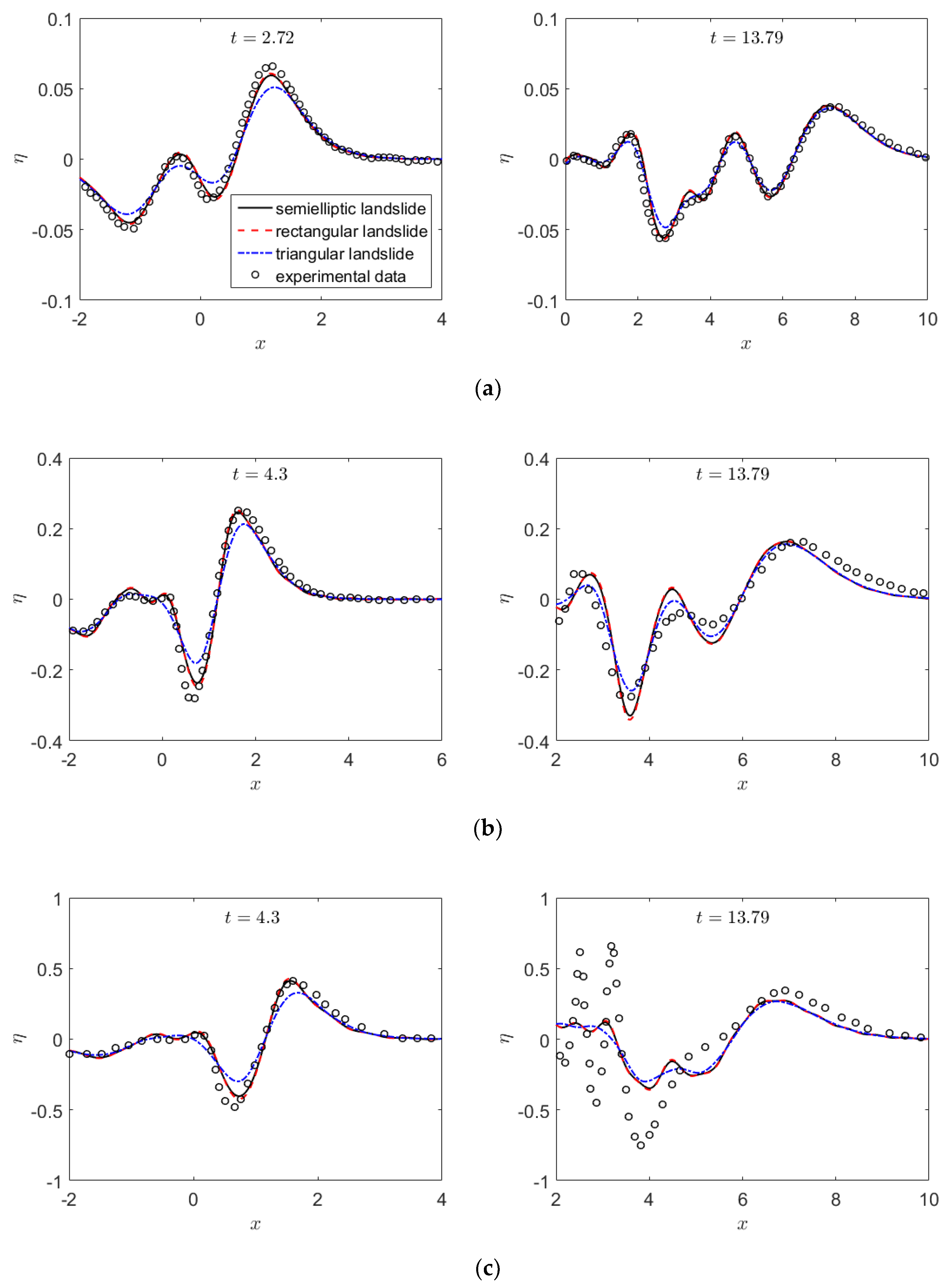
Figure 2 presents the comparisons of free surface elevations of the LFD model with three different landslide shapes and experimental data in different instants. Dimensionless variables are used in the figure and the following ones, which are defined as x = x / L s , t = t g / L s , and η = η / H s , while all asterisks are dropped for the sake of simplicity. It can be observed that the results of the LFD model with a semielliptical landslide agree well with the experimental data in both instants of runs 21 and 23 and t = 4.3 of run 24, while for t = 13.79 of run 24, the LFD model underpredicts the amplitude of both the leading wave crest and the oscillating waves behind it. The reason for this is that the nonlinear effect becomes more important with the increase of the landslide velocity (Fr = 0.5), as is pointed out in [51]. This demonstrates the validation of the numerical method and the accuracy of the LFD model. Besides, it can be found that in all three runs, the results obtained by the rectangular landslide also agree well with the ones obtained by the semielliptical landslide. However, the results produced by the triangular landslide display lower amplitudes of both crests and troughs at t = 2.72 for run 21 and t = 4.3 for runs 23 and 24, while as time increases (t = 13.79), the leading crests from all three landslide shapes tend to be similar, which is consistent with the findings in [35]. For the following crests and troughs, the results of the triangular landslide are still different to those of the rectangular and semielliptical landslides. For run 21, the landslide Froude number is Fr = 0.125, which is small enough for the linear model to be accurate. With the increase of the landslide Froude number (Fr = 0.375, 0.5 in runs 23 and 24), the amplitudes of the generated water waves increase so that the nonlinear effect becomes more important and the results obtained by the LFD model become worse. In conclusion, the LFD model is accurate enough for the problem with Fr ≤ 0.375. In the following section, six cases with different water depths and landslide Froude numbers are used to investigate the effects of landslide shapes on the leading crests generated. The maximum landslide Froude number is Fr = 0.375, so the LFD model is accurate enough, as is demonstrated above.

3. Results and Discussions

In this section, six more cases are used to investigate the effects of the landslide shape, water depth, and landslide Froude number on the propagation of water waves generated by a submerged landslide at a constant water depth. To evaluate the dispersive effects on the generated water waves, three different wave models, which are the LFD model, LWD model, and LND model, are employed, in which the LFD model is treated as the most accurate one. The aim of this section is: (1) to investigate whether the findings (that is, the far-field leading waves converge to the same result for landslides with different shapes and the same volume) is valid for different water depths and landslide velocities; and (2) to evaluate whether other models, such as the LWD model and the LND model, which are more commonly used to predict landslide tsunami hazards, can also reproduce this phenomenon.

3.1. Setup of Cases

We define the dimensionless parameters μ = h 0 / L c and F r = u t / g h 0 , where Hs is the maximum landslide thickness and Lc is the characteristic landslide length. For the three different shapes of landslide with the same enclosed area, we set Lc to be the length of a semielliptical landslide. The setups of the six cases are given in Table 1, where different relative water depths (μ) and landslide Froude numbers (Fr) are used. In cases 1, 2, and 3, the same landslide Fr is used and the relative water depths (μ) are increased from 0.1 to 0.6. In cases 4, 5, and 6, the relative water depths also increase from 0.1 to 0.6, but the landslide Fr number increases up to 0.375. For each case, three different landslide shapes are used in the simulation.

3.2. Effect of Water Depth on the Generated Leading Wave

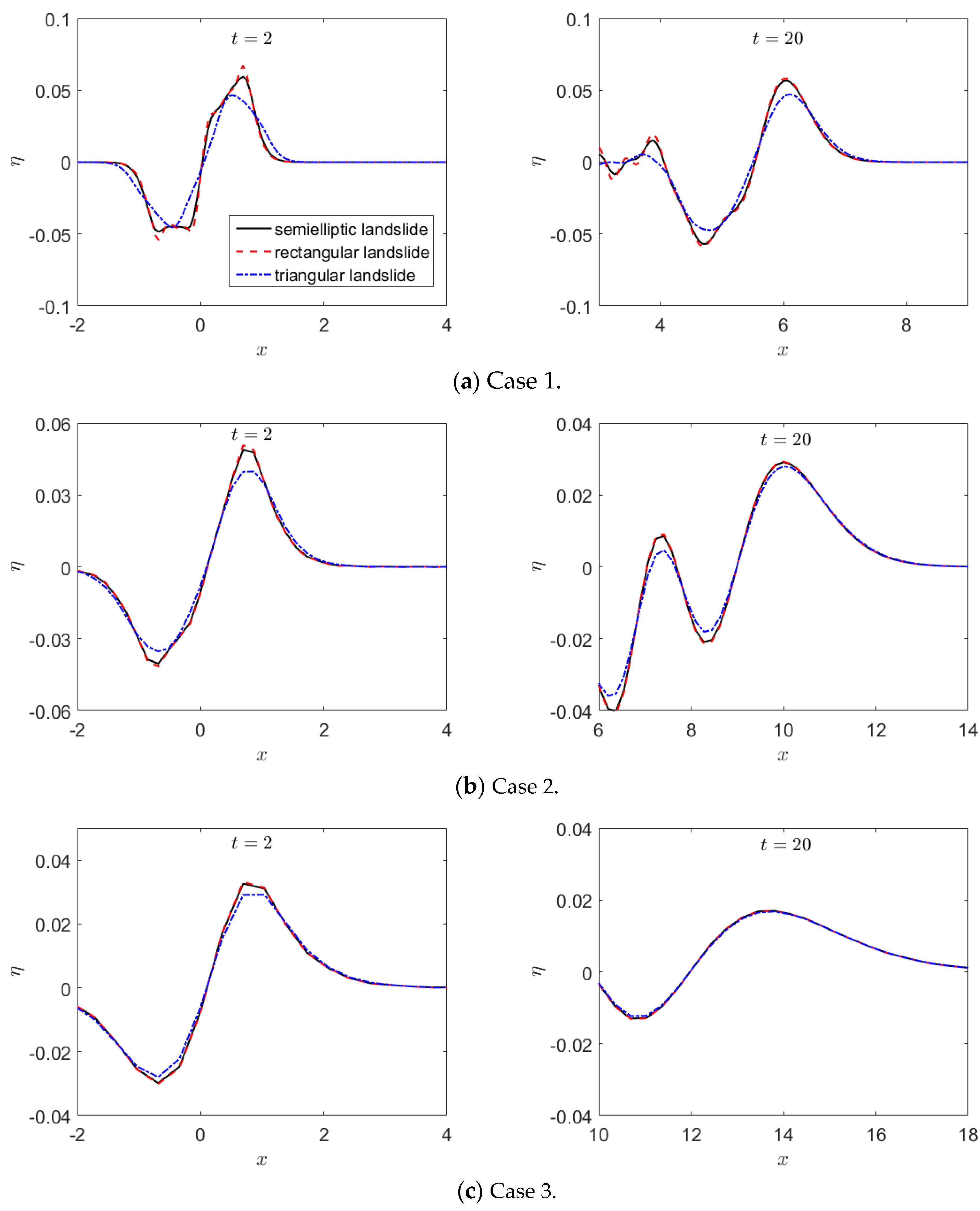
Figure 3 presents the comparisons of free surface elevations obtained by the LFD model for cases 1, 2, and 3. For these three cases, the landslide Fr number remains constant (Fr = 0.1), while the relative water depths increase from μ = 0.1 to 0.6. It should also be noted that in this section, dimensionless variables are used in all the figures, as in Figure 2. It can be observed that at instant t = 2 (corresponding to the initial wave field), the leading waves obtained by rectangular and semielliptical landslides with the same enclosed area in all three cases are very similar, while the magnitudes of the leading waves obtained by the triangular landslide for all three cases are smaller than those produced by rectangular and semielliptical landslides. Additionally, with the increase of the water depth (from cases 1 to 3), the leading waves obtained by the three different landslides tend to the same one. This indicates that the effects of landslide shapes on the generated waves are dependent on water depths.
As the time increases (t = 20), the leading wave generated by the triangular landslide in case 1 still differs obviously in comparison with those generated by rectangular and semielliptical landslides. However, as the water depth increases (cases 2 and 3), it can be found that the leading waves generated by all three landslides eventually converge to the same one, as is expected. It is well-known that for shallow water waves, the phase speed is c = g h 0 , where g is the gravitational acceleration and h0 is the water depth. Therefore, for a constant water depth, all the components of waves propagate with the same constant phase speed, which means that the leading wave keeps its shape during propagation. For deep water waves, the phase speed is c = g / k , where k is the wavenumber, which means that all the components of the waves propagate with different phase speeds, and finally the leading wave will change its shape during propagation. This is the frequency dispersion phenomenon, which may explain the findings in this study and those in [35].
In addition, it can be observed that both near-field and far-field leading waves obtained by rectangular and semielliptical landslides display only slight differences for a relative water depth μ 0.3 because the shapes of the two landslides are very similar, as can be found in Figure 1. At a relatively deeper water depth (μ = 0.6), the three shapes of landslides provide almost the same far-field leading wave profile.

3.3. Effect of the Landslide Fr Number on the Generated Leading Wave

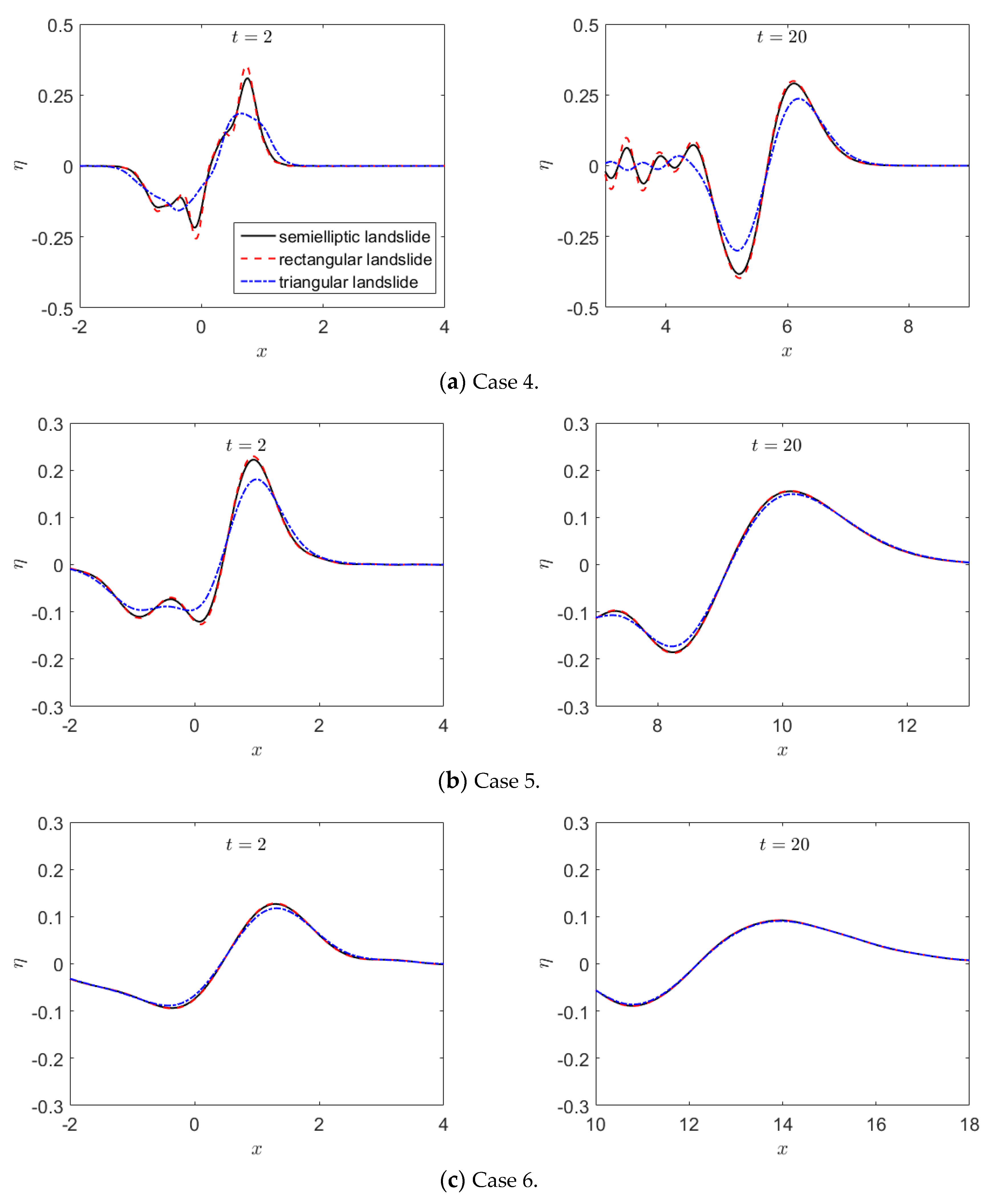
With the increase of the landslide Froude number (Fr = 0.375), similar results for water waves generated by three different landslides with different water depths are presented in Figure 4. It can be found that at a shallower water depth (case 4), both near-field and far-field leading waves obtained by the triangular landslide are different to those obtained by rectangular and semielliptical landslides with the same enclosed area. Additionally, the far-field leading waves obtained by three different landslides with the same volume converge to the same result in relatively deep water, which is similar to the findings in Figure 3. Compared with the three cases in Figure 3, it can be found that the increase of the landslide Froude number causes only higher amplitudes of the generated waves. This indicates that the phenomenon mentioned above is insensitive to the landslide Froude number.

3.4. Availability of LWD and LND models

LWD and LND models are more popular in the prediction of tsunami wave propagation due to their low computational cost. In this subsection, to evaluate the ability of these two models for correctly predicting the far-field leading waves, the results are compared against those obtained by the LFD model, which is the most accurate of the three models.
For the LWD model, the solution must also be calculated numerically, and the same method is used as in the LFD model. However, for the given motion of the landslide in Equation (12), the solution of the LND model can be obtained directly, as in [36], given by
η ( x , t ) = { η I S F ( x , t ) + η I S + ( x , t ) + η I S ( x , t ) 0 < t < T s η P S + ( x , t ) + η P S ( x , t ) t T s ,
where
{ η I S F ( x , t ) = F r 2 F r 2 1 h s ( x u t t ) η I S + ( x , t ) = 1 2 F r F r 1 h s ( x g h 0 t ) η I S ( x , t ) = 1 2 F r F r + 1 h s ( x + g h 0 t ) , F r 1 ,
{ η P S + ( x , t ) = 1 2 F r F r 1 [ h s ( x u t T s g h 0 ( t T s ) ) h s ( x g h 0 t ) ] η P S ( x , t ) = 1 2 F r F r + 1 [ h s ( x u t T s + g h 0 ( t T s ) ) h s ( x + g h 0 t ) ] , F r 1 .
Here, η I S + ( x , t ) and η P S + ( x , t ) denote the leading waves generated by the landslide before and after the landslide motion stops. From the solution, it can be found that the leading wave translates with a constant speed during propagation, and hence the leading wave will keep its shape all the way. It is well-known that the LND model is based on a shallow water assumption and is suitable for shallow water waves. This indicates that the finding showing that the far-field leading crest is independent of the exact shapes of the landslide but related to the enclosed area of the landslide cannot be reproduced by the LND model properly due to its lack of a dispersive effect.
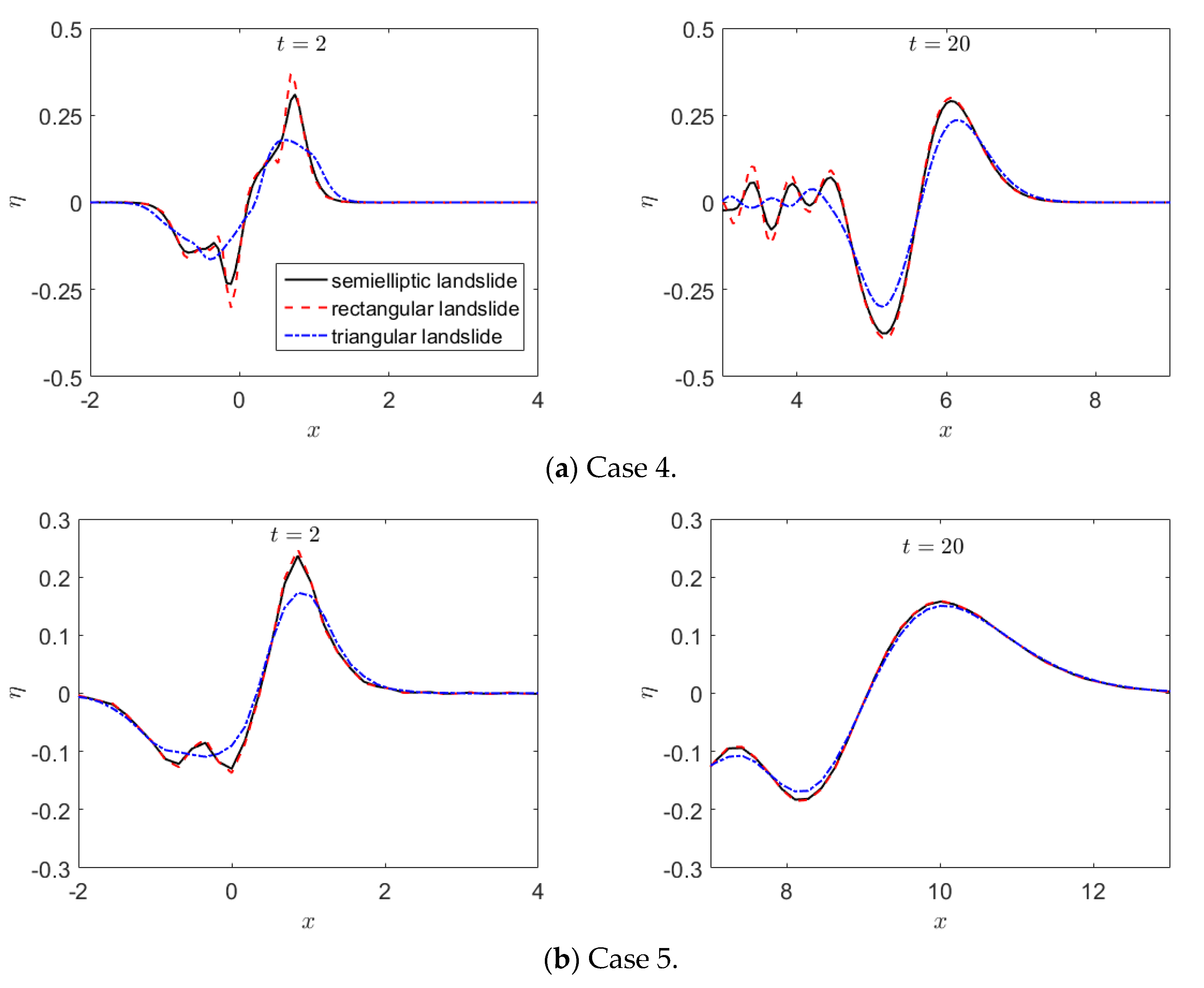
Figure 5 presents comparisons of the semielliptical landslide-generated waves produced by the three different models for different water depths. From the figure, it can be observed that for a shallower water depth (case 4), both the LWD and LND models can reproduce the near-field (t = 2) leading crest well, while as the time increases (t = 20), the leading crest changes its shape due to a dispersive effect and the LND model cannot reproduce the shape of the leading crest; however, it can predict the amplitude and phase velocity of the crest. The results obtained by the LWD model agree well with those obtained by the LFD model. As the water depth increases (cases 5 and 6), the dispersive effect becomes more important. It can be observed from the figure that the results obtained by the LND model deviate obviously from those obtained by the LFD model, as is expected. The LND model overpredicts the amplitude and phase velocity of the leading crest. However, owing to the inclusion of a weakly dispersive effect, the LWD model can predict the leading crest much better at different water depths, even in deep water (μ = 0.6 in case 6).
For the LWD model, the results of the leading crest generated by three different shapes of landslides are presented in Figure 6. It can be observed that the results agree well with those obtained by the LFD model (see Figure 4). As the water depth increases, the far-field leading crests obtained by the three different shapes of landslides converge to the same one. The LWD model can reproduce this phenomenon properly.

4. Conclusions

For water waves generated by a submerged landslide, an interesting phenomenon was recently found [35]; that is, the far-field leading wave over a constant depth is independent of the shapes of landslides but related to the enclosed area of the landslide. To clarify the effects of landslide shapes on the generated water waves at different water depths and the availability of different wave models to this phenomenon, three linear models developed in [45] were employed in this study: the LFD, LWD, and LND models. Three different landslide shapes with the same enclosed area in a one-dimensional problem were used, namely semielliptical, rectangular, and triangular shapes. Subsequently, the LFD model, which is the most accurate of the three models, was validated by comparing it against experimental data available. The effects of landslide shapes on the generated water waves at different water depths and landslide Fr numbers were then investigated by using the LFD model. Afterward, the availability of the other two models for this phenomenon was evaluated. The main conclusions can be summarized as follows:
(1)
The amplitudes of the generated water waves increase with the increase of the landslide Fr number. Up to Fr = 0.375, the nonlinear effect can be neglected and the LFD model has been demonstrated to be accurate enough;
(2)
From the analysis of the results obtained by the LFD model, it can be concluded that the phenomenon above is caused by frequency dispersion and will be invalid for landslide-generated water waves at a shallow water depth. The near-field leading waves in shallower water are sensitive to the shapes of landslides, while the far-field leading waves in deeper water are independent of the exact shapes of landslides. Specifically, the choice of a rectangular or semielliptical shape is not influential for a relative depth of μ ≥ 0.3, and at a deeper water depth (μ = 0.6), the leading waves obtained by all three different landslide shapes (triangular, rectangular, and semielliptical) are almost the same. In addition, the phenomenon mentioned above is insensitive to the landslide Froude number;
(3)
The LND model (based on a shallow water assumption), which is one of the most popular models for tsunami wave prediction, cannot be used to reproduce this phenomenon. However, the LWD model can predict the phenomenon properly. For leading wave propagation, the LWD model is demonstrated to be accurate enough up to at least μ = 0.6, although only weakly dispersive effects are included.
The findings of this study are useful for understanding the propagation of landslide-generated water waves (or tsunamis) and provide a guide for the selection of models for tsunami simulation. However, it should be pointed out that the results in this study are valid for a limited range of the landslide Fr numbers (0.1 and 0.375) and relative depths (0.1, 0.3, and 0.6). For practical tsunami waves propagating from offshore to coastal areas, the water depth decreases and nonlinearity will be important and must be properly taken into account.

Author Contributions

Conceptualization, H.J. and C.L.; methodology, H.J. and J.H.; validation, Y.G.; formal analysis, Y.G., H.J., and J.H.; investigation, Y.G. and H.J.; writing—original draft preparation, Y.G. and H.J.; writing—review and editing, C.L. and J.H.; funding acquisition, H.J. All authors have read and agreed to the published version of the manuscript.

Funding

This research was funded by the National Natural Science Foundation of China, grant number 51909211; Natural Science Basic Research Plan in Shaanxi Province of China, grant number 2019JQ-744; and Natural Science Foundation of Education Department of Shaanxi Province, China, grant number 19JK0591.

Conflicts of Interest

The authors declare no conflict of interest.

Appendix A. Derivation of the LFD Model

We start from the vertical two-dimensional governing equation of water waves; that is, the Laplace equation, which is given below:
2 Φ x 2 + 2 Φ z 2 = 0 ,
where x and z denote the horizontal and vertical coordinates, respectively, with z pointing upwards with its origin at the still water level, while Φ ( x , z ) is the velocity potential.
Linearized boundary conditions at the free surface (z = 0) are
η t Φ z = 0 ,
Φ t + g η = 0 ,
where g denotes the gravitational acceleration and η is the free surface elevation.
At the bottom z = h 0 , the linearized boundary condition is
Φ z = h s t ,
where h0 is the still water depth without a landslide and hs(x, t) is the landslide height.
Following the standard procedure of the Fourier and Laplace transforms, the transformed velocity potential can be readily obtained, as in [35], given by
Φ ˜ ¯ = F ˜ ¯ k s 2 sinh ( k z ) g k cosh ( k z ) s 2 cosh ( k h 0 ) + g k sinh ( k h 0 ) ,
where tilde and bar denote the Fourier and Laplace transforms, respectively. Additionally,
F ˜ ¯ = e i k x 0 e s t h s t d t d k ,
where ω 2 = g k tanh ( k h 0 ) is the dispersion relation. Substituting (A5) into the transformed dynamic boundary condition (Equation (A3)), we get
η ˜ ¯ = 1 cosh ( k h 0 ) s F ˜ ¯ s 2 + ω 2 .
Finally, by taking the inverse Fourier and Laplace transforms, the free surface elevation can be obtained as
η = 1 2 π e i k x cosh ( k h 0 ) 0 t F ˜ ( k , τ ) cos [ ω ( t τ ) ] d τ ,
where the convolution theorem has been used in the second integral above and F ˜ ( k , τ ) is defined by
F ˜ ( k , t ) = h ˜ s ( k ) [ ( i k d x 0 d t ) 2 i k d 2 x 0 d t 2 ] e i k x 0 ( t ) .
For a given landslide shape and motion, the solution for the free surface elevation (Equation (A8)) has to be integrated numerically.

References

  1. Renzi, E.; Sammarco, P. The hydrodynamics of landslide tsunamis: Current analytical models and future research directions. Landslides 2016, 13, 1369–1377. [Google Scholar] [CrossRef] [Green Version]
  2. Kulikov, E.A.; Rabinovich, A.B.; Thomson, R.E.; Bornhold, B.D. The landslide tsunami of November 3, 1994, Skagway Harbor, Alaska. J. Geophys. Res. Space Phys. 1996, 101, 6609–6615. [Google Scholar] [CrossRef]
  3. Manenti, S.; Amicarelli, A.; Todeschini, S. WCSPH with Limiting Viscosity for Modeling Landslide Hazard at the Slopes of Artificial Reservoir. Water 2018, 10, 515. [Google Scholar] [CrossRef] [Green Version]
  4. Manenti, S.; Pierobon, E.; Gallati, M.; Sibilla, S.; D’Alpaos, L.; Macchi, E.; Todeschini, S. Vajont Disaster: Smoothed Particle Hydrodynamics Modeling of the Postevent 2D Experiments. J. Hydraul. Eng. 2016, 142, 5015007. [Google Scholar] [CrossRef]
  5. Tappin, D.R.; Watts, P.; Grilli, S.T. The Papua New Guinea tsunami of 17 July 1998: Anatomy of a catastrophic event. Nat. Hazards Earth Syst. Sci. 2008, 8, 243–266. [Google Scholar] [CrossRef] [Green Version]
  6. Løvholt, F.; Pedersen, G.; Harbitz, C.B.; Glimsdal, S.; Kim, J. On the characteristics of landslide tsunamis. Philos. Trans. R. Soc. A Math. Phys. Eng. Sci. 2015, 373, 20140376. [Google Scholar] [CrossRef] [Green Version]
  7. Fine, I.; Rabinovich, A.; Bornhold, B.; Thomson, R.; Kulikov, E. The Grand Banks landslide-generated tsunami of November 18, 1929: Preliminary analysis and numerical modeling. Mar. Geol. 2005, 215, 45–57. [Google Scholar] [CrossRef]
  8. Fritz, H.M.; Hager, W.H.; Minor, H.-E. Landslide generated impulse waves. Exp. Fluids 2003, 35, 505–519. [Google Scholar] [CrossRef]
  9. Fritz, H.M.; Hager, W.H.; Minor, H.-E. Landslide generated impulse waves. 2. Hydrodynamic impact craters. Exp. Fluids 2003, 35, 520–532. [Google Scholar] [CrossRef]
  10. Harbitz, C.B.; Pedersen, G.; Gjevik, B. Numerical Simulations of Large Water Waves due to Landslides. J. Hydraul. Eng. 1993, 119, 1325–1342. [Google Scholar] [CrossRef]
  11. Heller, V.; Hager, W.H. Impulse Product Parameter in Landslide Generated Impulse Waves. J. Waterw. Port, Coastal Ocean Eng. 2010, 136, 145–155. [Google Scholar] [CrossRef]
  12. Heller, V.; Hager, W. Wave types of landslide generated impulse waves. Ocean Eng. 2011, 38, 630–640. [Google Scholar] [CrossRef]
  13. Kim, G.-B.; Cheng, W.; Sunny, R.C.; Horrillo, J.J.; McFall, B.C.; Mohammed, F.; Fritz, H.M.; Beget, J.; Kowalik, Z. Three Dimensional Landslide Generated Tsunamis: Numerical and Physical Model Comparisons. Landslides 2019, 1–17. [Google Scholar] [CrossRef]
  14. Manenti, S.; Wang, D.; Domínguez, J.M.; Li, S.; Amicarelli, A.; Albano, R. SPH Modeling of Water-Related Natural Hazards. Water 2019, 11, 1875. [Google Scholar] [CrossRef] [Green Version]
  15. Ataie-Ashtiani, B.; Yavari-Ramshe, S. Numerical simulation of wave generated by landslide incidents in dam reservoirs. Landslides 2011, 8, 417–432. [Google Scholar] [CrossRef]
  16. Behrens, J.; Dias, F. New computational methods in tsunami science. Philos. Trans. R. Soc. A Math. Phys. Eng. Sci. 2015, 373, 20140382. [Google Scholar] [CrossRef] [Green Version]
  17. Fritz, H.M.; Hager, W.H.; Minor, H.-E. Near Field Characteristics of Landslide Generated Impulse Waves. J. Waterw. Port Coastal, Ocean Eng. 2004, 130, 287–302. [Google Scholar] [CrossRef]
  18. Løvholt, F.; Harbitz, C.B.; Haugen, K.B. A parametric study of tsunamis generated by submarine slides in the Ormen Lange/Storegga area off western Norway. Mar. Pet. Geol. 2005, 22, 219–231. [Google Scholar] [CrossRef]
  19. Whittaker, C.; Nokes, R.; Davidson, M. Tsunami forcing by a low Froude number landslide. Environ. Fluid Mech. 2015, 15, 1215–1239. [Google Scholar] [CrossRef]
  20. Jamin, T.; Gordillo, L.; Ruiz-Chavarría, G.; Berhanu, M.; Falcon, E. Experiments on generation of surface waves by an underwater moving bottom. Proc. R. Soc. A Math. Phys. Eng. Sci. 2015, 471, 20150069. [Google Scholar] [CrossRef] [Green Version]
  21. Shokina, N.; Aizinger, V. On numerical modelling of impulse water waves generated by submarine landslides. Environ. Earth Sci. 2015, 74, 7387–7405. [Google Scholar] [CrossRef]
  22. Reymond, D.; Okal, E.A.; Hebert, H.; Bourdet, M. Rapid forecast of tsunami wave heights from a database of pre-computed simulations, and application during the 2011 Tohoku tsunami in French Polynesia. Geophys. Res. Lett. 2012, 39, 11603. [Google Scholar] [CrossRef] [Green Version]
  23. Dutykh, D.; Poncet, R.; Dias, F. The VOLNA code for the numerical modeling of tsunami waves: Generation, propagation and inundation. Eur. J. Mech. B Fluids 2011, 30, 598–615. [Google Scholar] [CrossRef] [Green Version]
  24. Lynett, P.; Liu, P. A numerical study of submarine–landslide–generated waves and run–up. Proc. R. Soc. A Math. Phys. Eng. Sci. 2002, 458, 2885–2910. [Google Scholar] [CrossRef]
  25. Ataie-Ashtiani, B.; Jilani, A.N. A higher-order Boussinesq-type model with moving bottom boundary: Applications to submarine landslide tsunami waves. Int. J. Numer. Methods Fluids 2007, 53, 1019–1048. [Google Scholar] [CrossRef]
  26. Fuhrman, D.R.; Madsen, P.A. Tsunami generation, propagation, and run-up with a high-order Boussinesq model. Coast. Eng. 2009, 56, 747–758. [Google Scholar] [CrossRef]
  27. Ruffini, G.; Heller, V.; Briganti, R. Numerical modelling of landslide-tsunami propagation in a wide range of idealised water body geometries. Coast. Eng. 2019, 153, 103518. [Google Scholar] [CrossRef]
  28. Gisler, G.R.; Weaver, R.; Gittings, M.L. SAGE calculations of the tsunami threat from La Palma. Sci. Tsunami Hazards 2006, 24, 288–301. [Google Scholar]
  29. Abadie, S.M.; Harris, J.; Grilli, S.T.; Fabre, R. Numerical modeling of tsunami waves generated by the flank collapse of the Cumbre Vieja Volcano (La Palma, Canary Islands): Tsunami source and near field effects. J. Geophys. Res. Space Phys. 2012, 117. [Google Scholar] [CrossRef]
  30. Ma, G.; Kirby, J.T.; Shi, F. Numerical simulation of tsunami waves generated by deformable submarine landslides. Ocean Model. 2013, 69, 146–165. [Google Scholar] [CrossRef]
  31. Li, G.; Chen, G.; Li, P.; Jing, H. Efficient and Accurate 3-D Numerical Modelling of Landslide Tsunami. Water 2019, 11, 2033. [Google Scholar] [CrossRef] [Green Version]
  32. Montagna, F.; Bellotti, G.; Di Risio, M. 3D numerical modeling of landslide-generated tsunamis around a conical island. Nat. Hazards 2011, 58, 591–608. [Google Scholar] [CrossRef]
  33. Lin, C.; Pastor, M.; Li, T.; Liu, X.; Qi, H.; Lin, C. A SPH two-layer depth-integrated model for landslide-generated waves in reservoirs: Application to Halaowo in Jinsha River (China). Landslides 2019, 16, 2167–2185. [Google Scholar] [CrossRef]
  34. Fu, L.; Jin, Y.-C. Investigation of non-deformable and deformable landslides using meshfree method. Ocean Eng. 2015, 109, 192–206. [Google Scholar] [CrossRef]
  35. Lo, H.-Y.; Liu, P. On the analytical solutions for water waves generated by a prescribed landslide. J. Fluid Mech. 2017, 821, 85–116. [Google Scholar] [CrossRef]
  36. Tinti, S.; Bortolucci, E. Energy of Water Waves Induced by Submarine Landslides. Pure Appl. Geophys. PAGEOPH 2000, 157, 281–318. [Google Scholar] [CrossRef]
  37. Liu, P.; Lynett, P.; Synolakis, C. Analytical solutions for forced long waves on a sloping beach. J. Fluid Mech. 2003, 478, 101–109. [Google Scholar] [CrossRef] [Green Version]
  38. Sammarco, P.; Renzi, E. Landslide tsunamis propagating along a plane beach. J. Fluid Mech. 2008, 598, 107–119. [Google Scholar] [CrossRef]
  39. Renzi, E.; Sammarco, P. The influence of landslide shape and continental shelf on landslide generated tsunamis along a plane beach. Nat. Hazards Earth Syst. Sci. 2012, 12, 1503–1520. [Google Scholar] [CrossRef] [Green Version]
  40. Madsen, P.A.; Hansen, A.B. Transient waves generated by a moving bottom obstacle: A new near-field solution. J. Fluid Mech. 2012, 697, 237–272. [Google Scholar] [CrossRef] [Green Version]
  41. Antuono, M.; Brocchini, M. The Boundary Value Problem for the Nonlinear Shallow Water Equations. Stud. Appl. Math. 2007, 119, 73–93. [Google Scholar] [CrossRef]
  42. Matteo, A.; Brocchini, M. Maximum run-up, breaking conditions and dynamical forces in the swash zone: A boundary value approach. Coast. Eng. 2008, 55, 732–740. [Google Scholar] [CrossRef]
  43. Antuono, M.; Brocchini, M. Swash Zone Dynamics due to Impulsive Waves. J. Waterw. Port Coastal, Ocean Eng. 2011, 137, 192–203. [Google Scholar] [CrossRef]
  44. Brocchini, M. A reasoned overview on Boussinesq-type models: The interplay between physics, mathematics and numerics. Proc. R. Soc. A Math. Phys. Eng. Sci. 2013, 469, 20130496. [Google Scholar] [CrossRef] [PubMed] [Green Version]
  45. Jing, H.X.; Chen, G.D.; Liu, C.G.; Wang, W.; Zuo, J.L. Dispersive effects of water waves generated by submerged landslide. Nat. Hazards 2020. Under review. [Google Scholar]
  46. Zitti, G.; Ancey, C.; Postacchini, M.; Brocchini, M. Impulse waves generated by snow avalanches: Momentum and energy transfer to a water body. J. Geophys. Res. Earth Surf. 2016, 121, 2399–2423. [Google Scholar] [CrossRef]
  47. Zitti, G.; Ancey, C.; Postacchini, M.; Brocchini, M. Snow avalanches striking water basins: Behaviour of the avalanche’s centre of mass and front. Nat. Hazards 2017, 88, 1297–1323. [Google Scholar] [CrossRef]
  48. Harbitz, C.B.; Løvholt, F.; Pedersen, G.; Masson, D.G. Mechanisms of tsunami generation by submarine landslides: A short review. Norw. J. Geol. 2006, 86, 255–264. [Google Scholar]
  49. Mohammed, F.; Fritz, H.M. Physical modeling of tsunamis generated by three-dimensional deformable granular landslides. J. Geophys. Res. Space Phys. 2012, 117, 11. [Google Scholar] [CrossRef] [Green Version]
  50. Rzadkiewicz, S.A.; Mariotti, C.; Heinrich, P. Numerical Simulation of Submarine Landslides and Their Hydraulic Effects. J. Waterw. Port Coastal, Ocean Eng. 1997, 123, 149–157. [Google Scholar] [CrossRef]
  51. Whittaker, C. Modelling of Tsunami Generated by the Motion of a Rigid Block along a Horizontal Boundary. Ph.D. Thesis, University of Canterbury, Christchurch, New Zealand, 2013. [Google Scholar]
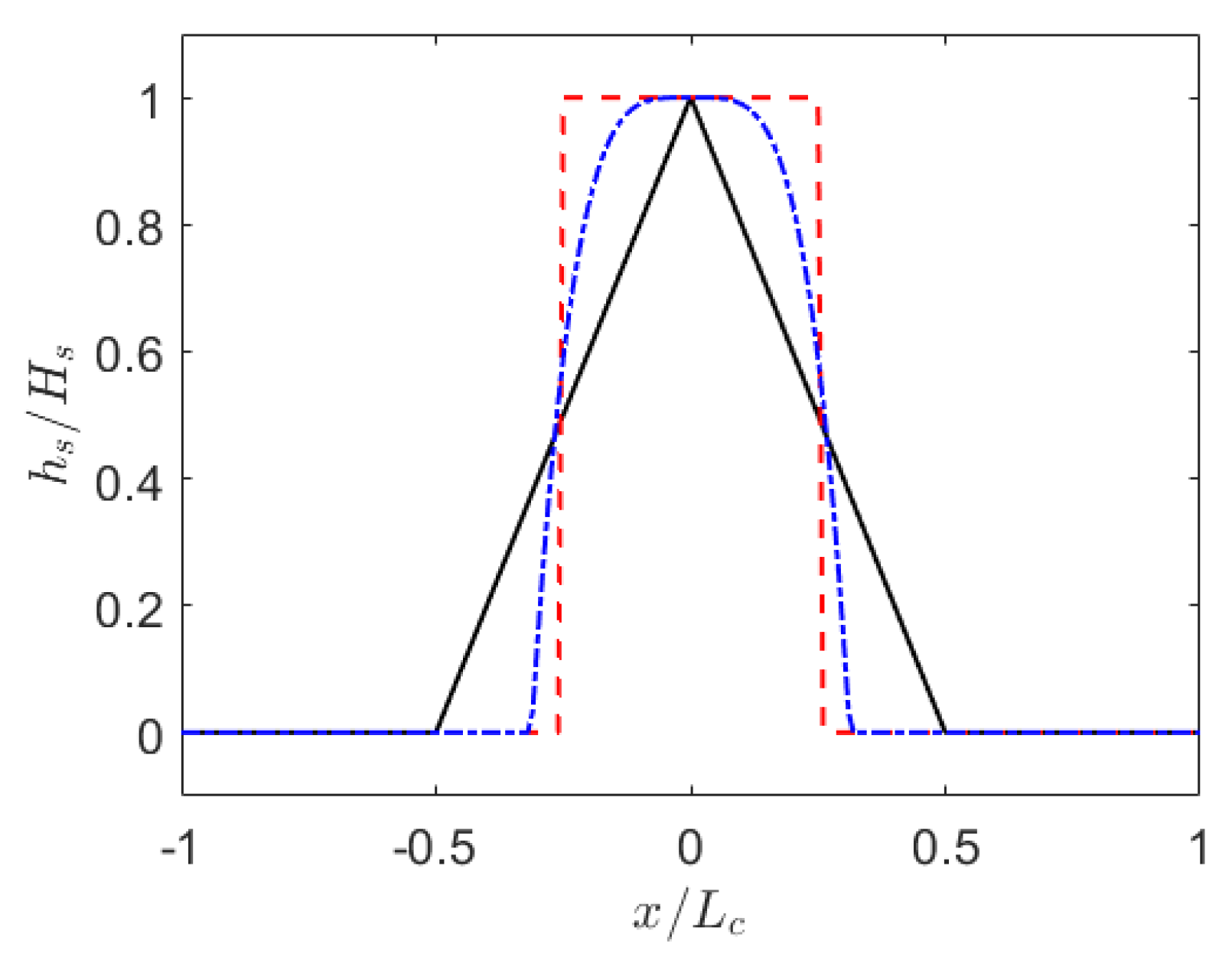
Figure 1. Three different shapes of landslide.
Jmse 08 00196 g001
Figure 2. Comparisons of free surface elevations obtained by the linear fully dispersive (LFD) model and experimental data in [51] (note that dimensionless variables are used).
Jmse 08 00196 g002
Figure 3. Comparisons of water waves generated by landslides with three different shapes (Fr = 0.1, LFD model).
Jmse 08 00196 g003
Figure 4. Comparisons of water waves generated by landslides with three different shapes (Fr = 0.375, LFD model).
Jmse 08 00196 g004aJmse 08 00196 g004b
Figure 5. Comparisons of semielliptical landslide-generated water waves obtained by three models.
Jmse 08 00196 g005
Figure 6. Comparisons of water waves generated by landslides with three different shapes (Fr = 0.375, linear weakly dispersive (LWD) model).
Jmse 08 00196 g006
Table 1. Setup of the cases.
Caseh0 (m)Hs (m)Lc (m)ut (m/s)μFr
10.1750.0261.750.1310.10.1
20.1750.0260.580.1310.30.1
30.1750.0260.290.1310.60.1
40.1750.0261.750.4910.10.375
50.1750.0260.580.4910.30.375
60.1750.0260.290.4910.60.375