Improving Coastal Ocean Wave Height Forecasting during Typhoons by using Local Meteorological and Neighboring Wave Data in Support Vector Regression Models

Abstract

This study is aimed at applying support vector regression to perform real-time typhoon wave height forecasting with lead times of 1 to 3 h. Two wave rider buoys in the coastal ocean northeast of Taiwan provided real-time observation wave and meteorological data for the study. Information from actual typhoon events was collected and used for model calibration and validation. Three model structures were developed with different combinations of input variables, including wave, typhoon, and meteorological data. Analysis of forecasting results indicated that the proposed models have good generalization ability, but forecasts with longer lead times underestimate extreme wave heights. Comparisons of models with different inputs indicated that adding local meteorological data enhanced forecasting accuracy. Backup models were also developed in case local wave and meteorological data were unavailable. Analysis of these models revealed that when local wave heights are unknown, using neighboring wave heights can improve forecasting performance.

1. Introduction

Severe waves caused by typhoons are major threats to both beach management and safe navigation. Wave forecasting during typhoons can provide useful information for authorities in planning and preparing for resource allocation to reduce the risk to human life and property and mitigate coastal disasters.

Wave hindcasting and forecasting have been central topics in coastal engineering for decades. Early on, empirical regression methods [1,2,3,4] were proposed to predict wave parameters such as wave height and period. These methods are generally based on the wind–wave relationship and use the inputs of wind speed, wind direction, wind duration, and fetch length to predict ocean waves. Empirical regression methods suffer from the limitation that ocean waves are generated by complex processes which involve not only the wind field but also bathymetric effects and the wave generation process [5]. Later, as a result of improved computer efficiency and knowledge of the physical wave formation process, numerical methods based on the wind–wave energy spectrum were proposed to forecast wave characteristics [6,7,8,9,10,11]. Numerical models that account for the physical interaction between wave parameters and their driving forces are competent for wave calculation. However, they require a large amount of preparatory work, such as collecting bathymetric data, and forecasts can be delayed due to the considerable time required for data collection and processing [12,13]. Moreover, numerical models were reported to be insufficient for forecasting extreme situations [5].

Artificial intelligence and machine learning methods that have low computational cost and are easy to implement have been adopted in hydrologic forecasting. Among the various methods, artificial neural networks (ANNs) [14,15,16,17], support vector machines (SVMs) [18,19,20,21,22], and fuzzy inference models (FIMs) [23,24,25,26,27] are commonly and successfully used for forecasting various hydrologic variables. Regarding wave forecasting, ANNs were used by Deo and Sridhar Naidu [28], Tsai et al. [29], and Mandal and Prabaharan [30] to forecast wave heights with inputs of present and previous wave heights. Deo et al. [31] applied ANNs to forecast wave height and period by using the generated wind speeds as inputs. Chang et al. [5] used an ANN model to refine the wave calculations of a numerical model by using simulated wind speed and wave height from the numerical model. Moreover, Kazeminezhad et al. [32] and Mahjoobi et al. [33] applied an FIM to hindcast wave height and period in Lake Ontario by using wind field data. Özger and Şen [34] explored the relationship between wave height and wind speed and applied an FIM to forecast the significant wave height at the California coast. SVMs have also been applied in wave hindcasting and forecasting. Mahjoobi and Mosabbeb [35] used an SVM to simulate the significant wave height for Lake Michigan by using current and previous wind speed data as inputs. Elbisy [36] combined an SVM and a genetic algorithm to predict the significant wave height, wave direction, and peak spectral period in a coastal zone near the Nile delta.

Although machine learning methods are often used to perform wave hindcasting and forecasting, few studies have applied machine learning methods to forecast waves induced by typhoons. Chang and Chien [37,38] applied an ANN model and a hybrid fuzzy-neural model to simulate typhoon wave height by adopting typhoon moving speed and location data. Tsai et al. [39] used hurricane location, pressure, and intensity in an ANN model to forecast wave heights along a ship route during hurricanes. Wei [40] used an ANN and an SVM to predict typhoon-induced wave height near coastal areas in northeast Taiwan. Chen [41] developed a probabilistic forecasting method using an SVM and an FIM to perform probabilistic wave height forecasting during typhoon warning periods. The abovementioned studies forecasted typhoon waves using only typhoon and wave data. When meteorological data in the study area are available, it is logical to deduce that adding these data can improve wave forecasting performance.

This study applied support vector regression (SVR) to develop various typhoon wave forecasting models by using different sets of typhoon, wave, and meteorological data. Two wave rider buoys in the coastal ocean of northeast Taiwan provided wave and meteorological data for the study. Typhoon data were available from typhoon warnings issued when typhoons were projected to hit Taiwan. Different sets of input variables were used to form three wave forecasting model structures. Real-time wave height forecasting with lead times of 1 to 3 h was performed for predicting typhoon events. Validation results proved that adding local meteorological data can improve wave forecasting performance. Moreover, backup models that do not use local wave and meteorological data to perform wave forecasting were also developed. Results from evaluation of the models revealed that when local wave and meteorological data are unavailable, using neighboring wave data can enhance forecasting performance.

2. Support Vector Regression

An SVM was proposed by Vapnik [42,43] on the basis of the structural risk minimization induction principle, which aims to minimize actual error in the validation phase. SVM was originally developed to solve the classification problem but was later proposed for use with regression applications. The SVR algorithm is introduced as follows [44,45,46].

The construction of the SVR function uses a supervised learning method in which input and output data are assigned before the model is built. Let $x$ be the input vector and $y$ be the output variable. Given a dataset [($x_1$,$y_1$), ($x_2$,$y_2$), …, ($x_n$,$y_n$)], the SVR function is constructed by using a nonlinear function $\mathsf{\Phi }\left(x\right)$.

$$f\left(x\right)=w·\mathsf{\Phi }\left(x\right)+b$$

(1)

where $w$ is the weight vector, $b$ is bias, and $\mathsf{\Phi }$ is a nonlinear function that maps the original data onto a higher dimensional feature space where the input and output data can exhibit linearity. SVR differs from traditional regressions in the calibration process defined by Vapnik’s ε-insensitive loss function $L_{\epsilon }$.

$$L_{\epsilon }\left(y_i\right)=\{\begin{array}{cc}0,& \mathrm{for}\left|y_i-\left[w·\mathsf{\Phi }\left(x_i\right)+b\right]\right|<\epsilon \\ \left|y_i-\left[w·\mathsf{\Phi }\left(x_i\right)+b\right]\right|-\epsilon ,& \mathrm{for}\left|y_i-\left[w·\mathsf{\Phi }\left(x_i\right)+b\right]\right|\ge \epsilon \end{array}$$

(2)

The loss function tolerates an error that is less than $\epsilon$. Therefore, the data within the extent of the ε-tube have no loss. Only data outside the ε-tube are penalized by the ε-insensitive loss function. This regression problem can be expressed as the following optimization problem based on the theory of structural risk minimization.

$$\begin{array}{c}\underset{w,b,{\mathsf{\xi }}_i^{+},{\mathsf{\xi }}_i^{-}}{\min }\hspace{1em}\frac{1}{2}{w}^{\mathrm{T}}·w+C·{{{\displaystyle \sum }}^{}}_{i=1}^n\left({\mathsf{\xi }}_i^{+}+{\mathsf{\xi }}_i^{-}\right)\hfill \\ \mathrm{subject}\mathrm{to} y_i-\left[w·\mathsf{\Phi }\left(x_i\right)+b\right]\le \epsilon +{\mathsf{\xi }}_i^{+} \hfill \\ \hspace{1em}\left[w·\mathsf{\Phi }\left(x_i\right)+b\right]-y_i\le \epsilon +{\mathsf{\xi }}_i^{-}\hfill \\ \hspace{1em}{\mathsf{\xi }}_i^{+}, {\mathsf{\xi }}_i^{-}\ge 0,\hspace{1em}i=1,2, \dots ,n,\hfill \end{array}$$

(3)

where ${\mathsf{\xi }}_i^{+}$ and ${\mathsf{\xi }}_i^{-}$ are slack variables respectively indicating the upper and lower training errors subject to error tolerance $\epsilon$, and $C$ is a positive cost constant that determines the level of penal loss when a training error occurs. By introducing a set of two Lagrange multipliers, ${\mathsf{\alpha }}_i^{+}$ and ${\mathsf{\alpha }}_i^{-}$, a quadratic programming algorithm can be adopted to solve the optimization problem as follows:

$$\begin{array}{c}\underset{{\mathsf{\alpha }}_i^{+},{\mathsf{\alpha }}_i^{-}}{\max }\hspace{1em}{{\displaystyle \sum }}_{i=1}^n{y}_i\left({\mathsf{\alpha }}_i^{+}-{\mathsf{\alpha }}_i^{-}\right)-\mathsf{\epsilon }·{{\displaystyle \sum }}_{i=1}^n\left({\mathsf{\alpha }}_i^{+}+{\mathsf{\alpha }}_i^{-}\right)\hfill \\ \hspace{1em}\hspace{1em}-\frac{1}{2}{{{\displaystyle \sum }}^{}}_{i,j=1}^n\left({\mathsf{\alpha }}_i^{+}-{\mathsf{\alpha }}_i^{-}\right)({\mathsf{\alpha }}_j^{+}-{\mathsf{\alpha }}_j^{-})\mathsf{\Phi }{\left(x_i\right)}^{\mathrm{T}}·\mathsf{\Phi }\left(x_j\right) \hfill \\ \mathrm{subject}\mathrm{to}\hspace{0.17em}{{\displaystyle \sum }}_{i=1}^n\left({\mathsf{\alpha }}_i^{+}-{\mathsf{\alpha }}_i^{-}\right)=0\hfill \\ \hspace{1em}\hspace{1em}0\le {\mathsf{\alpha }}_i^{+},{\mathsf{\alpha }}_i^{-}\le C, i=1,2, \dots ,n.\hfill \end{array}$$

(4)

After the determination of the Lagrange multipliers, parameters $w$ and $b$ of the SVR function can be estimated under Karush–Kühn–Tucker complementarity conditions. As a result, the SVR function can be formulated as follows:

$$f\left(x\right)={{\displaystyle \sum }}_{i,j=1}^n\left({\mathsf{\alpha }}_i^{+}-{\mathsf{\alpha }}_i^{-}\right)\mathsf{\Phi }{\left(x_i\right)}^{\mathrm{T}}·\mathsf{\Phi }\left(x_j\right)+b.$$

(5)

The inner products in the equation can be calculated in a simple form by using a kernel function $K\left(x_i,x\right)$:

$$K\left(x_i,x\right)=\mathsf{\Phi }{\left(x_i\right)}^{\mathrm{T}}·\mathsf{\Phi }\left(x\right).$$

(6)

Commonly used kernels in SVR include linear, polynomial, sigmoid, and radial basis functions. Dibike et al. [47] described the advantages that the radial basis function has over other kernels. Moreover, several studies [36,48,49] have demonstrated the superior capability of the radial basis function for hydrologic and wave forecasting. Therefore, this study used the radial basis function kernel with a parameter $\gamma$ as the kernel function:

$$K\left(x_i,x\right)=\exp (-\gamma {\left|x_i-x\right|}^2).$$

(7)

With the use of the kernel function, the SVR function can be reformulated as

$$f\left(x\right)={{\displaystyle \sum }}_{i=1}^n\left({\mathsf{\alpha }}_i^{+}-{\mathsf{\alpha }}_i^{-}\right)K\left(x_i,x\right)+b.$$

(8)

According to this equation, only data corresponding to nonzero Lagrange multipliers ${\overline{\alpha }}_i=\left({\mathsf{\alpha }}_i^{+}-{\mathsf{\alpha }}_i^{-}\right)$ can effectively be used to construct the SVR function. The data on the margin or outside the ε-insensitive tube have nonzero coefficients ${\overline{\alpha }}_i$. Therefore, these data are support vectors that support the construction of the regression function. Finally, the SVR function can be expressed as follows:

$$f\left(x\right)={{\displaystyle \sum }}_{k=1}^m{\overline{\alpha }}_k·K\left(x_k,x\right)+b$$

(9)

where $x_k$ denotes the support vector and $m$ is the number of support vectors. The parameters of the SVR to be calibrated are the cost constant $C$, error tolerance $\epsilon$, and kernel parameter $\gamma$. In this study, an exhausted grid search method was used to determine the parameters.

3. Wave and Meteorological Data

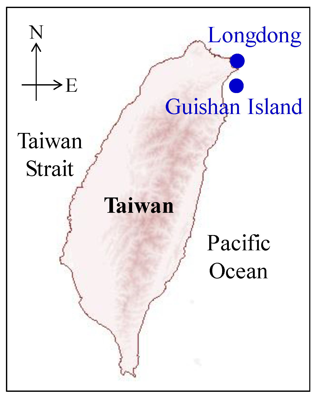
Taiwan is located in the west part of the North Pacific. Approximately four typhoons hit Taiwan annually, most of which move from the Pacific Ocean toward the east coast of Taiwan, as revealed by the long-term statistics of typhoon tracks. Government agencies have installed wave rider buoys to collect real-time observations of wave and meteorological data around the coastal ocean of Taiwan. This study used data from two nearby wave rider buoys in northeast Taiwan (Figure 1). The Longdong Buoy, installed by the Central Weather Bureau, is near the Longdong headland. The location of the buoy is 121.923° E and 25.096° N, approximately 1 km from the coast at a water depth of roughly 23 m. The Guishan Island Buoy, installed by the Tourism Bureau, is between the east coast of Taiwan and Guishan Island, which is approximately 10 km east of Taiwan. The Guishan Island Buoy, located at 121.923° E and 24.847° N with a water depth of roughly 28 m, is approximately 1 km west of Guishan Island and 9 km east of the coast of Taiwan.

The buoys measure both wave and meteorological data at hourly time steps. The wave data include significant wave height, significant wave period, peak period, and wave direction. The meteorological data include wind speed, wind direction, gust speed, air pressure, and air temperature. These data buoys are operated and maintained by the Coastal Ocean Monitoring Center, National Cheng Kung University with a real-time data quality control procedure [50] to ensure the quality of observed meteorological and wave data.

When a typhoon is expected to strike Taiwan, the Central Weather Bureau issues typhoon warnings. A sea warning is typically issued every 3 h when the typhoon is still distant. A land warning is issued once each hour when the perimeter of a typhoon is forecasted to hit the island of Taiwan within 18 h. Typhoon information, including central pressure, central wind velocity, instantaneous maximum gust, cyclonic radius, and center location (latitude and longitude), can be obtained from typhoon warnings. Hourly typhoon data are generally available because land warnings are usually issued when a typhoon is near and during landfall. Before a land warning is issued, typhoon data are only available from sea warnings at 3 h intervals. For this period, a linear interpolation scheme was applied to obtain hourly typhoon data. Generally, these interpolated data are a small portion of the total data for a typhoon event, at the beginning of hourly time series.

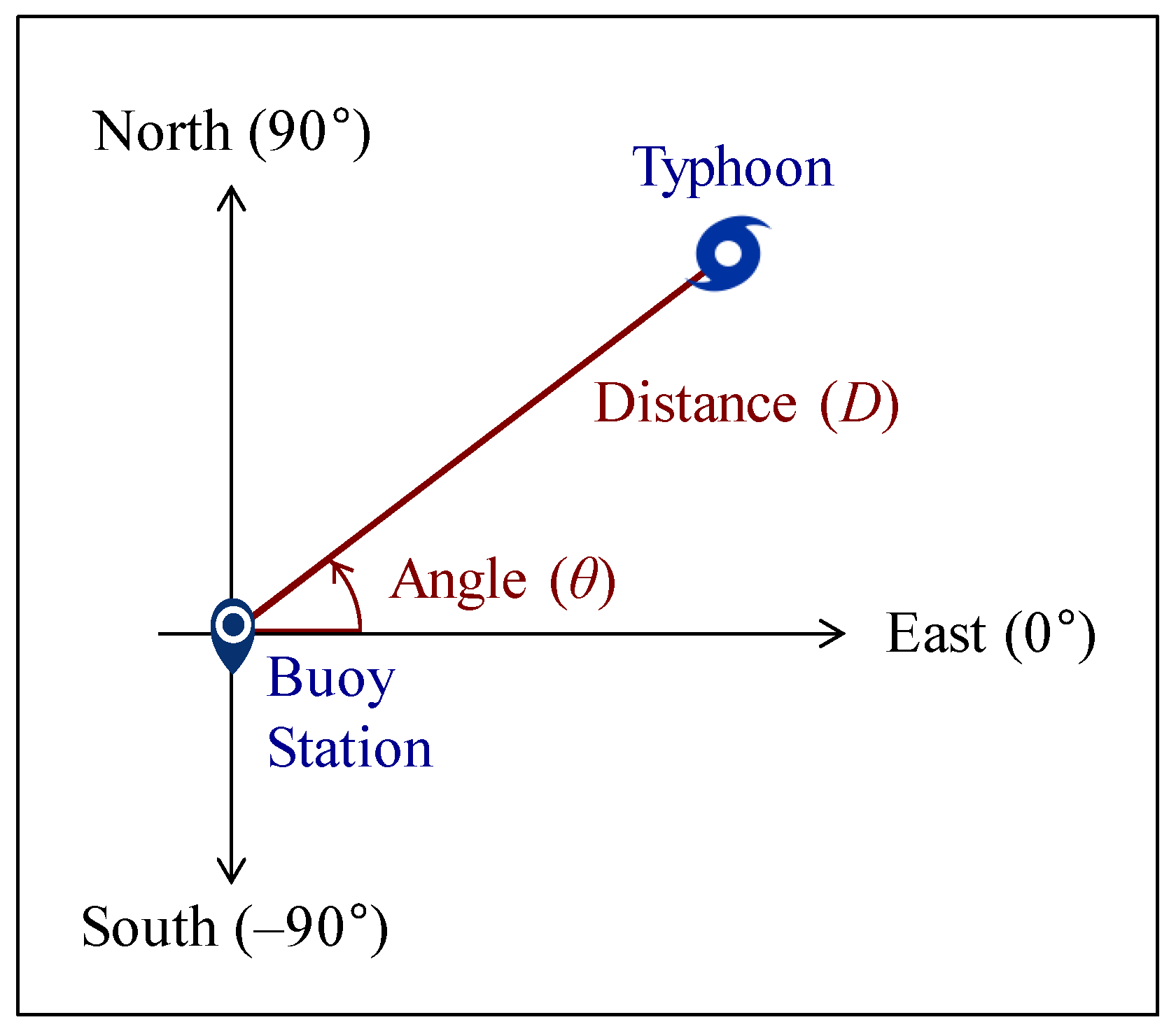
The center of a typhoon is expressed using latitude and longitude. To identify the position of a typhoon relative to a buoy site, latitude and longitude were transformed using a polar coordinate system, with the location of the buoy set as the origin. The position of the typhoon is thus defined using the great-circle distance ($D$) and angle ($\theta$). The angle facing the east is set as 0°, and the counterclockwise direction is set as positive (Figure 2). This definition of angle was applied following the scheme proposed by Chen [41] because typhoons generally approach Taiwan from the east and a typhoon north or south of the buoy has diverse effects on wave development. Additionally, this setting prevents discontinuity when the angle is ± 180° in the west, at which point the typhoon has passed.

Hourly meteorological and wave data from 2008 to 2016 were collected from two buoys. Hourly typhoon data were available from typhoon warnings. Finally, 17 typhoon events with complete buoy observations and typhoon data were obtained.

Table 1. Typhoon events and wave data.

Event No.	Name of Typhoon	Date (yyyy/mm/dd)	Lowest Pressure of Typhoon (hPa)	Max. Wave Height at Longdoong (cm)	Max. Wave Height at Guishan Island (cm)	No. of Data
1	Kalmaegi	2008/07/16	970	314	408	58
2	Fungwong	2008/07/26	948	793	603	73
3	Morakot	2009/08/05	955	818	551	208
4	Parma	2009/10/03	945	479	352	171
5	Namtheun	2010/08/30	995	110	156	22
6	Lionrock	2010/08/31	990	190	206	43
7	Meranti	2010/09/09	990	138	193	26
8	Fanapi	2010/09/17	940	721	617	64
9	Songda	2011/05/27	920	470	604	37
10	Doksuri	2012/06/28	995	152	174	28
11	Jelawat	2012/09/27	910	523	416	43
12	Usagi	2013/09/19	910	339	373	63
13	Fungwong	2014/09/19	985	339	373	73
14	Matmo	2014/07/21	960	427	685	55
15	Linfa	2015/07/06	975	194	177	67
16	Nepartak	2016/07/06	905	364	383	73
17	Megi	2016/09/25	940	1247	1039	67

lists the following information on these events: typhoon name, date on which the first warning was issued, the lowest central pressure of the typhoon, maximum wave height at Longdong, maximum wave height at Guishan Island, and number of hourly data points during the typhoon warning period. The first 12 events, with 836 data points (hourly data), were used for model calibration, and the remaining 5, with 335 data points, were used to validate the proposed model.

4. Model Development and Forecasting

4.1. Input Variable Determination

The SVR wave forecasting model aims to forecast significant wave heights ($H$) with lead times of 1 to 3 h. Input variables were determined to establish the model. According to the available data, the candidate input variables could be grouped into three categories: wave, typhoon, and meteorological variables. Both subjective and objective methods were used. The objective method was a correlation analysis, in which correlation coefficients between wave height at time t and lagged variables at time t – 1 to t – 3 were calculated. Variables that had a higher correlation with the wave height ($H$) were appropriate for use as input variables. Because model parsimony was also a key concern, expert knowledge was employed as the subjective method to remove redundant information and variables with lower correlation.

Wave data include wave height, wave period, peak period, and wave direction. Lagged wave height ($H$), having the highest correlation, was used as an input variable. Other wave data with lower correlation were unnecessary. Typhoon data include central pressure, central wind velocity, instantaneous maximum gust, cyclonic radius, and center location. The position and moving track of a typhoon have substantial influences on wave development. Therefore, the distance ($D$) and angle ($\theta$) of a typhoon relative to the buoy site were used as input variables. For the other four typhoon variables, cyclonic radius ($R$) and central wind velocity ($V$) had larger correlation coefficients (0.39 to 0.49 for $R$, and 0.24 to 0.33 for $V$) with wave height ($H$) than did instantaneous maximum gust and central pressure (0.22 to 0.31 and −0.22 to −0.28, respectively). Therefore, typhoon radius ($R$), wind velocity ($V$), distance ($D$), and angle ($\theta$) were used as input variables.

The meteorological data collected by the buoys included wind speed, wind direction, gust speed, air pressure, and air temperature. The correlations of wave height ($H$) with wind speed, gust speed, air pressure, and air pressure difference between the buoy site and typhoon center were calculated. Although gust speed had slightly higher correlation coefficients (0.61 to 0.74) than did wind speed (0.60 to 0.68), wind speed ($S$) was selected as the input variable because gust is a more temporary phenomenon and may have a weaker physical correlation to wave height ($H$) than wind speed ($S$). Air pressure ($P$) at the buoy site had a negative correlation with wave height ($H$), with correlation coefficients of −0.44 to −0.57. However, the difference in air pressure between a buoy site and a typhoon center had small correlation coefficients (−0.11 to 0.13) with wave height ($H$). Therefore, air pressure ($P$) was adopted as an input variable. As a result, the meteorological variables used in the forecasting model were wind speed ($S$) and air pressure ($P$).

All variables were normalized before being used in the model because different variables have different values and units that are not in the same order of magnitude. The variables of wave height ($H$), typhoon radius ($R$), typhoon central wind velocity ($V$), distance ($D$), wind speed at buoy ($S$), and air pressure at buoy ($P$) were linearly normalized to the interval [0, 1] by their respective minimum and maximum values in the calibration data set. Angle ($\theta$) data were linearly normalized into the interval of [−1, 1] corresponding to the original value of [−180°, 180°]. Thus, the original outputs of the model were normalized data. These outputs were then transformed into forecasted wave heights at their real scale.

4.2. Model Development

Three types of model structure were developed to forecast typhoon wave heights. The first model structure (M1) uses observed wave height ($H$) and typhoon variables ($R$, $V$, $D$, $\theta$) to forecast wave heights with lead times of 1 to 3 h. The M1 models are formulated as follows:

$$\widehat{H}\left(t+1\right)=f_{\mathrm{M}1\_1}\left[H\left(t\right), R\left(t\right),V\left(t\right), D\left(t\right), \theta \left(t\right)\right]$$

(10)

$$\widehat{H}\left(t+2\right)=f_{\mathrm{M}1\_2}\left[H\left(t\right), R\left(t\right),V\left(t\right), D\left(t\right), \theta \left(t\right)\right]$$

(11)

$$\widehat{H}\left(t+3\right)=f_{\mathrm{M}1\_3}\left[H\left(t\right), R\left(t\right),V\left(t\right), D\left(t\right), \theta \left(t\right)\right]$$

(12)

where $\widehat{H}$ is the forecasted wave height, $t$ is the time index, and $f_{\mathrm{M}1\_1}$, $f_{\mathrm{M}1\_2}$, and $f_{\mathrm{M}1\_3}$ indicate the SVR wave height forecasting models of M1 with lead times of 1, 2, and 3 h, respectively. The M1 model structure was regarded as a base model that simply adopts typhoon variables to forecast future wave height. Because there are two buoy stations, Longdong and Guishan Island, two corresponding sets of M1 models were developed.

The second model structure (M2) added local meteorological variables into M1. The forecasting models were formulated as

$$\widehat{H}\left(t+1\right)=f_{\mathrm{M}2\_1}\left[H\left(t\right), R\left(t\right),V\left(t\right), D\left(t\right), \theta \left(t\right), S\left(t\right), P\left(t\right)\right]$$

(13)

$$\widehat{H}\left(t+2\right)=f_{\mathrm{M}2\_2}\left[H\left(t\right), R\left(t\right),V\left(t\right), D\left(t\right), \theta \left(t\right), S\left(t\right), P\left(t\right)\right]$$

(14)

$$\widehat{H}\left(t+3\right)=f_{\mathrm{M}2\_3}\left[H\left(t\right), R\left(t\right),V\left(t\right), D\left(t\right), \theta \left(t\right), S\left(t\right), P\left(t\right)\right]$$

(15)

where $f_{\mathrm{M}2\_1}$, $f_{\mathrm{M}2\_2}$, and $f_{\mathrm{M}2\_3}$ represent the forecasting models of M2 with lead times of 1, 2, and 3 h, respectively. The M2 models with local wind and air pressure information were expected to achieve better forecasting performance than the M1 models, because local meteorological variables have considerable effects on wave formation.

Neighboring wave height data may also provide sea state information and enhance forecasting performance. This study used wave height from the other buoy station ($H_o$) as an additional input variable to establish M3 models:

$$\widehat{H}\left(t+1\right)=f_{\mathrm{M}3\_1}\left[H\left(t\right), R\left(t\right),V\left(t\right), D\left(t\right), \theta \left(t\right), S\left(t\right), P\left(t\right),H_o\left(t\right)\right]$$

(16)

$$\widehat{H}\left(t+2\right)=f_{\mathrm{M}3\_2}\left[H\left(t\right), R\left(t\right),V\left(t\right), D\left(t\right), \theta \left(t\right), S\left(t\right), P\left(t\right),H_o\left(t\right)\right]$$

(17)

$$\widehat{H}\left(t+3\right)=f_{\mathrm{M}3\_3}\left[H\left(t\right), R\left(t\right),V\left(t\right), D\left(t\right), \theta \left(t\right), S\left(t\right), P\left(t\right),H_o\left(t\right)\right]$$

(18)

where $f_{\mathrm{M}3\_1}$, $f_{\mathrm{M}3\_2}$, and $f_{\mathrm{M}3\_3}$ specify the forecasting models of M3 with lead times of 1, 2, and 3 h, respectively. For forecasting the wave heights at Longdong, the $H_o$ variable indicates the wave height at Guishan Island. Likewise, to forecast the wave heights at Guishan Island, the $H_o$ variable designates the wave height at Longdong.

In total, 18 models were to be calibrated (three model structures, each with three lead times, for two sites). Data from 12 calibration events were used to calibrate the SVR parameters, namely the cost constant $C$, error tolerance $\epsilon$, and kernel parameter $\gamma$. The grid search method was used to determine the parameter values. Root mean squared error (RMSE) was used as the objective function:

$$\mathrm{RMSE}=\sqrt{\frac{{{\displaystyle \sum }}_{i=1}^n{\left(H_i-{\widehat{H}}_i\right)}^2}{n}}$$

(19)

where $n$ is the number of data points. The parameter $C$ is less sensitive than parameters $\epsilon$ and $\gamma$. Hence, the grid size for $C$ is set as a large value; grid sizes for $\epsilon$ and $\gamma$ are much smaller. That is, the parameter calibration process emphasized tuning $\epsilon$ and $\gamma$ to reach the minimum RMSE values. The resulting optimal parameter values for the 18 SVR models are summarized as follows. The cost constant $C$ is 10 for all models. 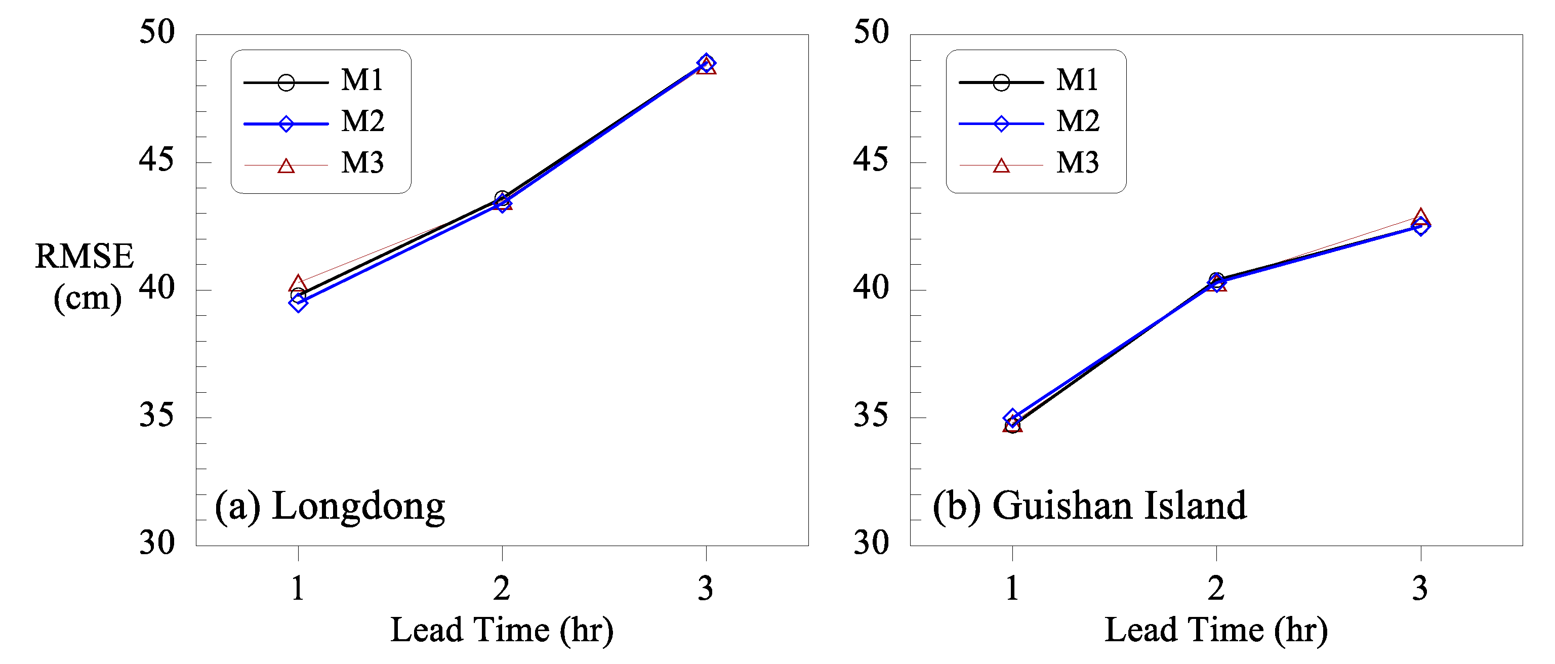The error tolerance $\epsilon$ ranges from 0.002 to 0.030, and the kernel parameter $\gamma$ ranges from 0.01 to 0.85. The RMSE values regarding calibration data are represented in Figure 3. Overall, M1, M2, and M3 had similar performance during the calibration phase, but the calibrated models for Guishan Island had smaller errors than those for Longdong. Obviously, model performance decreases as lead time increases.

4.3. Forecasting Results and Discussion

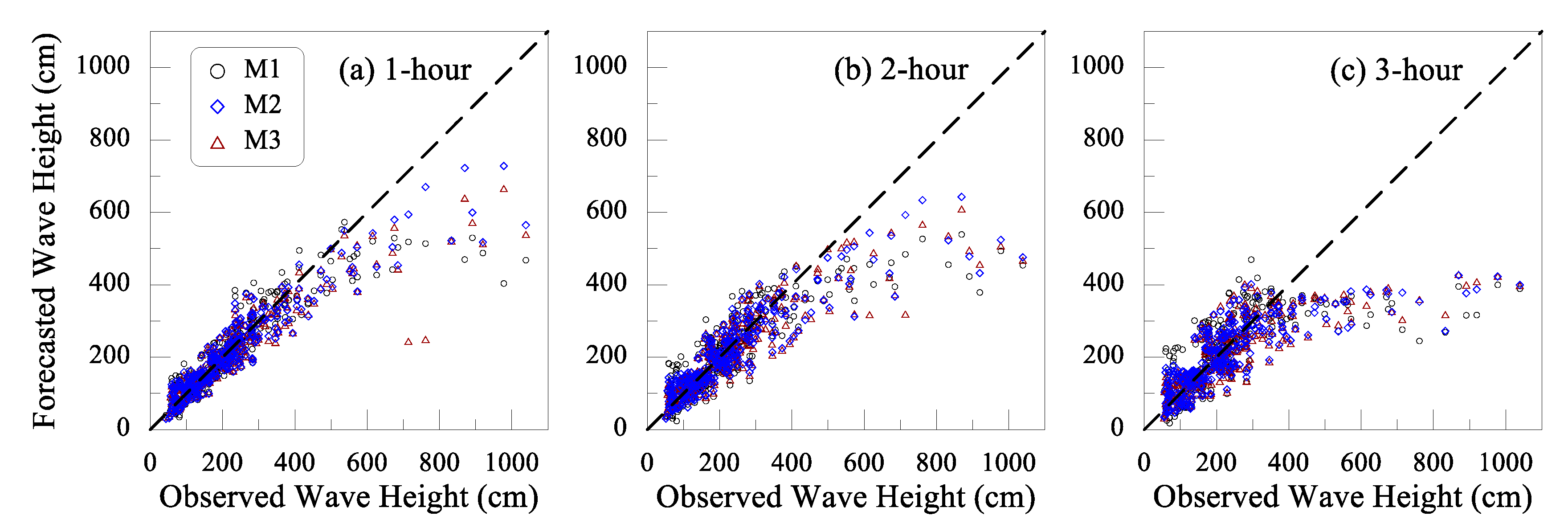
The developed SVR models were used to perform real-time wave height forecasting of validation events. Figure 4 and Figure 5 present scatter diagrams of the forecasting results for Longdong and Guishan Island, respectively. The forecasting results for the lead time of 1 h were satisfactory. For 2- and 3-h forecasting, the forecasts for large wave heights were obviously underestimated, especially the 3-h forecasting at Guishan Island. As for the M1, M2, and M3 models, the data of M2 and M3 are closer to the 45-degree line than those of M1, indicating that the addition of input variables can improve forecasting performance.

Quantitative indices were used to assess the model performance. One is the RMSE, and the other is the coefficient of efficiency (CE).

$$\mathrm{CE}=1-\frac{{{\displaystyle \sum }}_{i=1}^n{(H_i-{\widehat{H}}_i)}^2}{{{\displaystyle \sum }}_{i=1}^n{\left(H_i-\overline{H}\right)}^2}$$

(20)

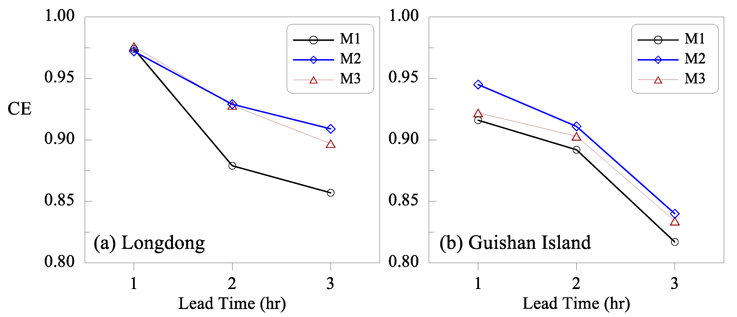
where $\overline{H}$ is the average observed wave height. A CE value closer to unity indicates better forecasting performance. Figure 6 and Figure 7 display the RMSE and CE values, respectively. With RMSE, M2 and M3, which are analogous, were more accurate than M1. Using CE, M2 and M3 also outperformed M1. Upon closer investigation, although M2 and M3 are comparable, M2 is slightly better than M3, with lower RMSEs and larger CEs overall. This indicates that adding local meteorological data can enhance forecasting performance. However, adding a variable that describes a neighboring wave state is unhelpful. Presumably, when added local meteorological data provides enough signals for wave formation, the heights of nearby waves are no longer informative. Moreover, during the calibration phase, the forecasting models for Guishan Island had better performance than those for Longdong. However, during the validation phase, the forecasting models for Longdong outperformed those for Guishan Island. This suggests that the models exhibit a tendency of overfitting for Guishan Island.

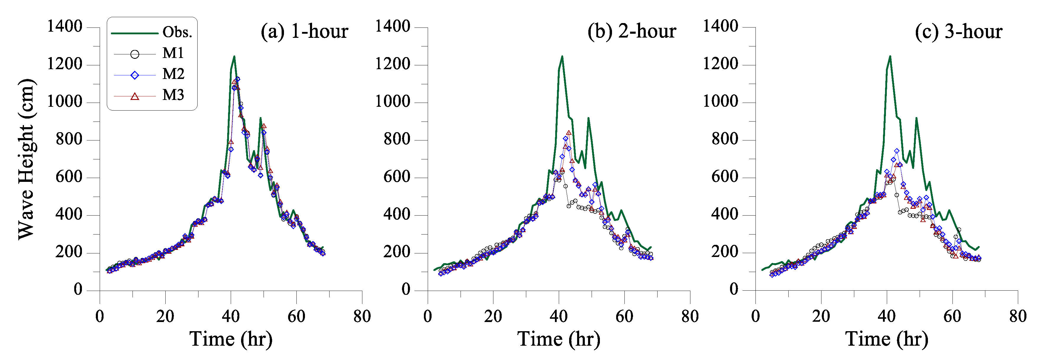
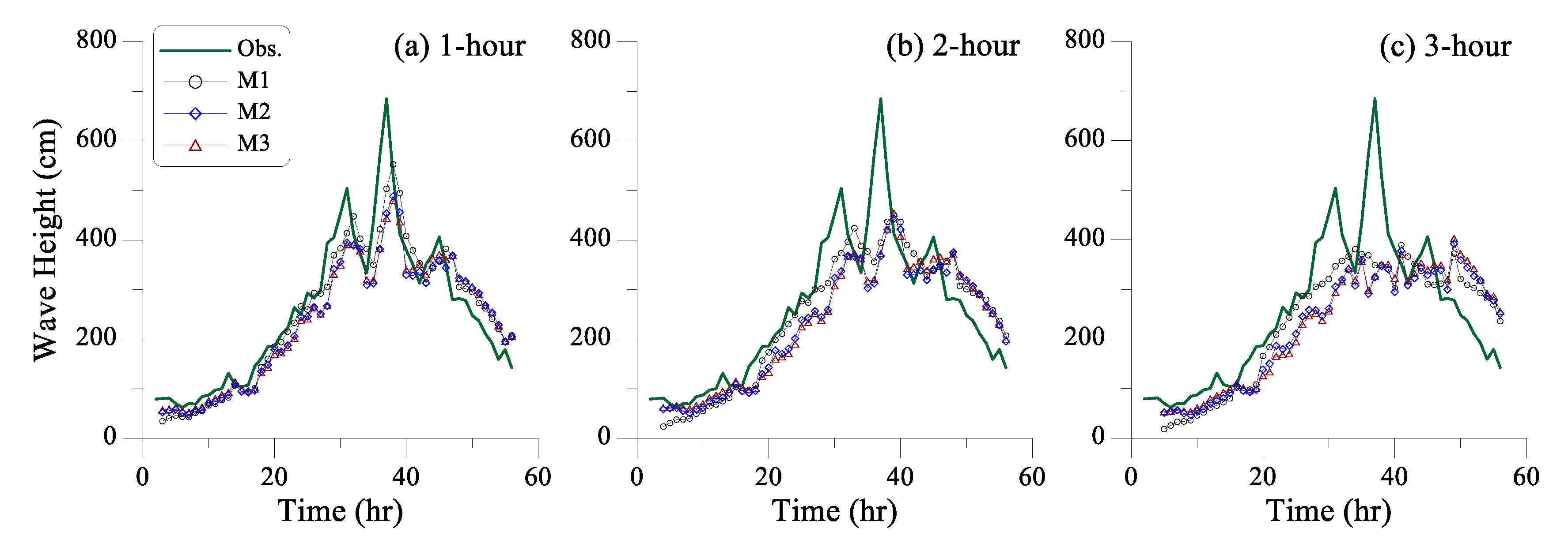
Figure 8 and Figure 9 present the hydrographs of wave height for the largest event (Event 17) at Longdong and the second largest (Event 14) at Guishan Island, respectively. One-hour forecasts are satisfactory, with minor underestimation for peak wave heights. For forecasts with longer lead times, the underestimation is obvious. Events 14 and 17 were large events with extreme wave heights around the peak greater than the calibration data. Therefore, these extreme data were never observed by the forecasting models. Although satisfactory 1-h forecasting results exhibit the generalization ability of the models, the ability of the models to extrapolate forecasts with longer lead times remains limited. Overall, adding local meteorological data can enhance the forecasting accuracy of SVR models to forecast wave height during typhoons, but the models imperfectly forecast extreme cases for longer lead times.

4.4. Backup System

In a practical implementation of real-time typhoon wave height forecasting, buoy data may be inaccessible due to failure in measuring devices or communication. In such cases, when real-time observation wave height and meteorological data are unavailable, the forecasting models cannot operate properly. Therefore, this study developed a backup system that does not require local wave and meteorological data to perform a real-time forecasting task. Two types of backup systems were developed. The first backup system, termed B1, uses only typhoon variables as the model inputs:

$$\widehat{H}\left(t+1\right)=f_{\mathrm{B}1\_1}\left[R\left(t\right),V\left(t\right), D\left(t\right), \theta \left(t\right)\right]$$

(21)

$$\widehat{H}\left(t+2\right)=f_{\mathrm{B}1\_2}\left[R\left(t\right),V\left(t\right), D\left(t\right), \theta \left(t\right)\right]$$

(22)

$$\widehat{H}\left(t+3\right)=f_{\mathrm{B}1\_3}\left[R\left(t\right),V\left(t\right), D\left(t\right), \theta \left(t\right)\right]$$

(23)

where $f_{\mathrm{B}1\_1}$, $f_{\mathrm{B}1\_2}$, and $f_{\mathrm{B}1\_3}$ indicate the forecasting models of B1 with lead times of 1, 2, and 3 h, respectively. The second backup system, B2, adopts the wave height from the neighboring buoy station ($H_o$) as an additional input variable.

$$\widehat{H}\left(t+1\right)=f_{\mathrm{B}2\_1}\left[R\left(t\right),V\left(t\right), D\left(t\right), \theta \left(t\right),H_o\left(t\right)\right]$$

(24)

$$\widehat{H}\left(t+2\right)=f_{\mathrm{B}2\_2}\left[R\left(t\right),V\left(t\right), D\left(t\right), \theta \left(t\right),H_o\left(t\right)\right]$$

(25)

$$\widehat{H}\left(t+3\right)=f_{\mathrm{B}2\_3}\left[R\left(t\right),V\left(t\right), D\left(t\right), \theta \left(t\right),H_o\left(t\right)\right]$$

(26)

where $f_{\mathrm{B}2\_1}$, $f_{\mathrm{B}2\_2}$, and $f_{\mathrm{B}2\_3}$ specify the forecasting models of B2 with lead times of 1, 2, and 3 h, respectively.

Calibration events provided data for determining the SVR forecasting model parameters regarding B1 and B2. The cost constant $C$ is 10 for all models. Error tolerance $\epsilon$ ranges from 0.003 to 0.024, and the kernel parameter $\gamma$ ranges from 0.42 to 0.90. The established models regarding calibration data have RMSEs ranging from 42.6 to 66.0 cm, which is larger than the RMSEs of the M1, M2, and M3 models overall (cf. Figure 3). 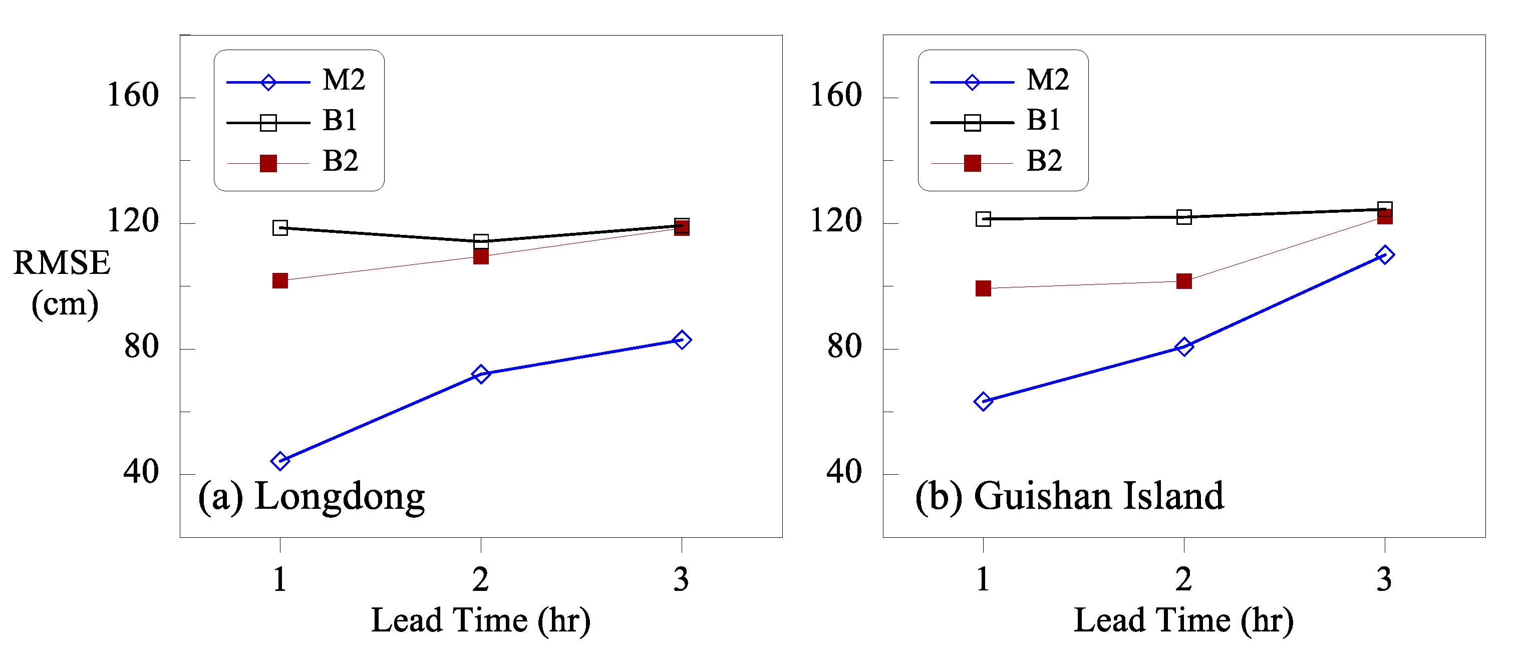For validation events, Figure 10 shows that the B1 and B2 models have RMSEs of approximately 100 to 120 cm; in the figure, the RMSEs of M2 models act as benchmarks to evaluate the performance of the backup systems. 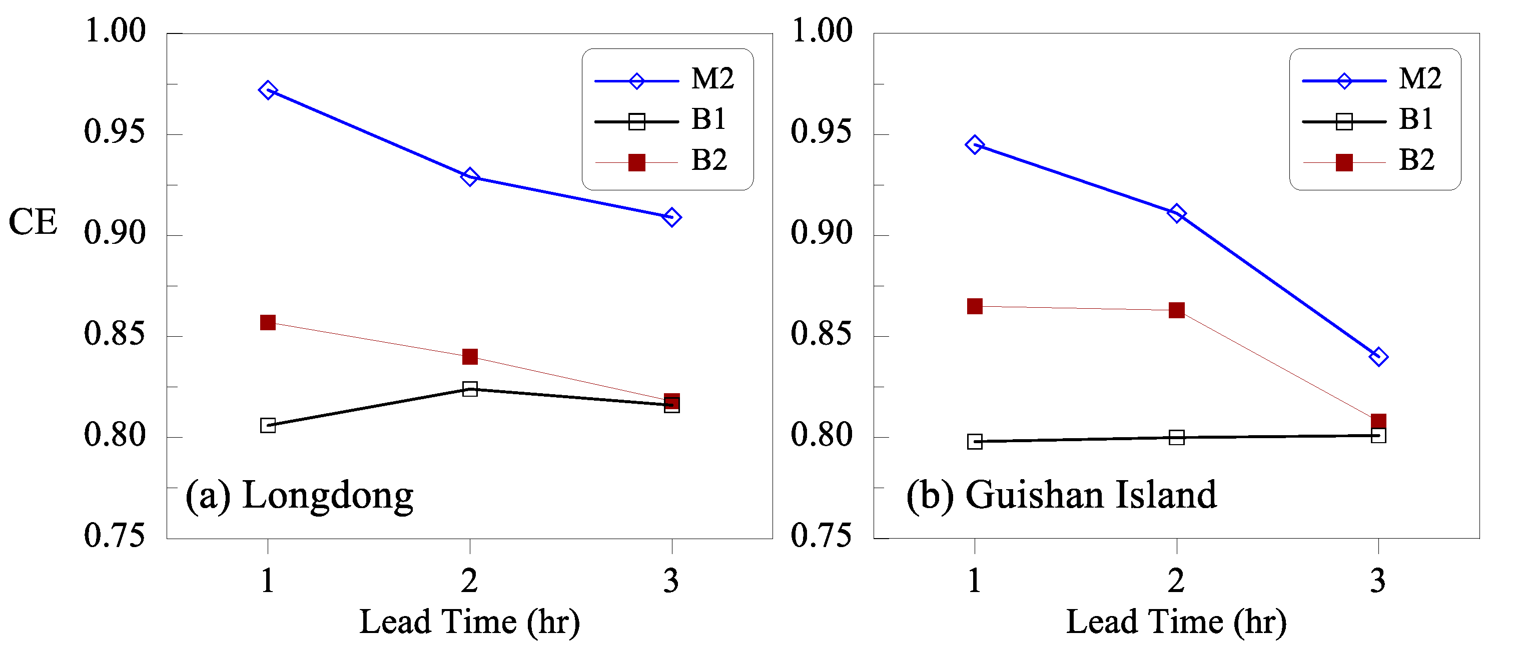Figure 11 presents the CEs for the B1 and B2 models; the CEs are roughly 0.80 to 0.86. Overall, the two backup systems are inferior to the original systems (M1, M2, and M3) but still have acceptable forecasting ability, with wave height forecast errors of approximately 1 m during typhoons. The B2 models outperformed the B1 models, indicating that when no local wave or meteorological data are available, adding neighboring sea state information (i.e., wave height) can enhance forecasting ability. However, as the lead time increases to 3 h, this enhancement becomes less apparent. 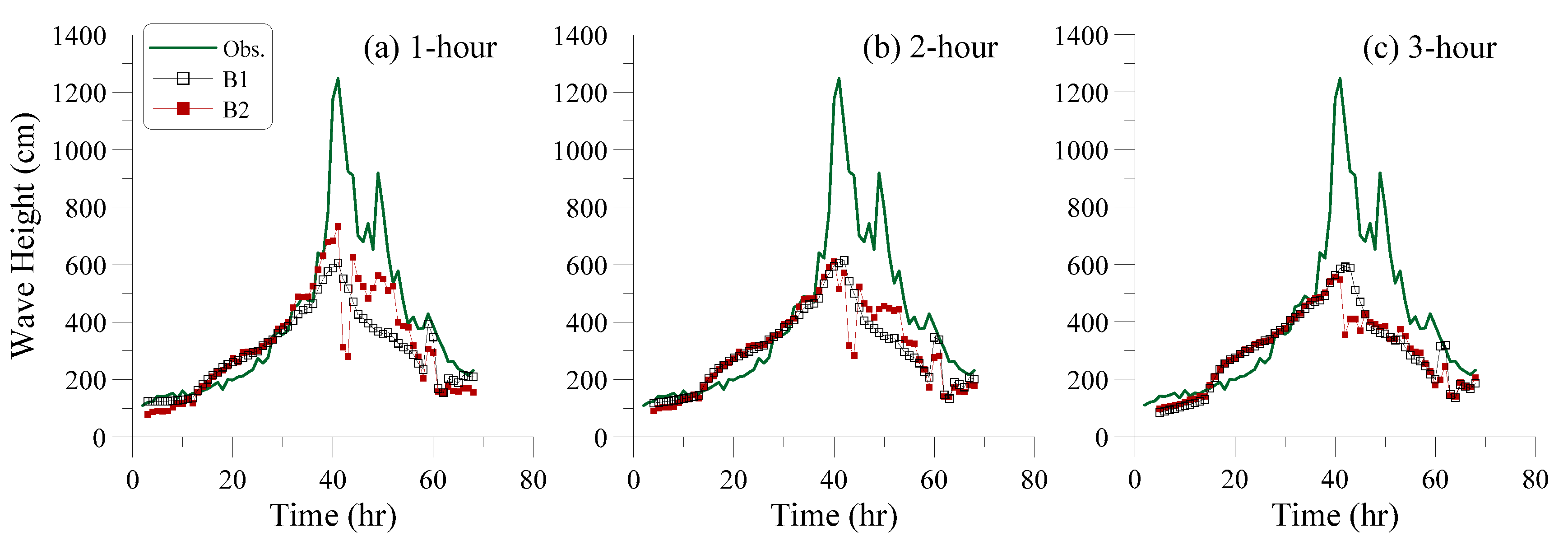Figure 12 illustrates the wave height forecasts made by the models for Event 17. Although the forecasts around extreme wave heights were underestimated, the models captured the tendency in wave height variation. The B1 and B2 models, without local wave and meteorological information, can reasonably forecast wave heights with small and normal magnitudes.

5. Conclusions

This study applied SVR in real-time typhoon wave height forecasting with lead times of 1 to 3 h. Various model structures were developed with different combinations of input variables, including wave, typhoon, and meteorological data. The coastal ocean in northeast Taiwan, where two buoys were installed to observe real-time wave and meteorological data, served as the study area. This study used 12 typhoon events to develop the forecasting models and 5 events to validate and compare the models’ performance.

Generally, the forecasting results for the lead time of 1 h are satisfactory, but in 2 and 3 h forecasting, the models underestimate extreme wave heights. A comparison of the M1, M2, and M3 models indicated that adding meteorological variables can improve forecasting accuracy but that adding another neighboring wave height variable cannot further enhance the forecasting accuracy. The generalization ability of the proposed models was verified by their ability to forecast extreme wave heights with the 1-h lead time, but the ability of the models to extrapolate forecasting for longer lead times remains limited. This study also developed two backup models in case real-time wave and meteorological data are unavailable. Although the backup models offer inferior performance compared with the original models, they possess an acceptable capability to forecast typhoon wave heights. A comparison of the backup systems revealed that when no local wave or meteorological data are available, adding neighboring wave height information can enhance forecasting performance. Overall, the study concludes that (1) using local meteorological data can improve wave height forecasting and (2) using neighboring wave heights can improve forecasting accuracy when the local wave heights are unknown.