Development of An Integrated Numerical Model for Simulating Wave Interaction with Permeable Submerged Breakwaters Using Extended Navier–Stokes Equations

Abstract

An integrated two-dimensional vertical (2DV) model was developed to investigate wave interactions with permeable submerged breakwaters. The integrated model is capable of predicting the flow field in both surface water and porous media on the basis of the extended volume-averaged Reynolds-averaged Navier–Stokes equations (VARANS). The impact of porous medium was considered by the inclusion of the additional terms of drag and inertia forces into conventional Navier–Stokes equations. Finite volume method (FVM) in an arbitrary Lagrangian–Eulerian (ALE) formulation was adopted for discretization of the governing equations. Projection method was utilized to solve the unsteady incompressible extended Navier–Stokes equations. The time-dependent volume and surface porosities were calculated at each time step using the fraction of a grid open to water and the total porosity of porous medium. The numerical model was first verified against analytical solutions of small amplitude progressive Stokes wave and solitary wave propagation in the absence of a bottom-mounted barrier. Comparisons showed pleasing agreements between the numerical predictions and analytical solutions. The model was then further validated by comparing the numerical model results with the experimental measurements of wave propagation over a permeable submerged breakwater reported in the literature. Good agreements were obtained for the free surface elevations at various spatial and temporal scales, velocity fields around and inside the obstacle, as well as the velocity profiles.

1. Introduction

Porous structures are constructed along coasts for shoreline protection and beach erosion prevention against wave attack. Permeable submerged breakwater is one of the artificial structures that reduce the impact of waves and currents to beaches without affecting aesthetic aspects of coastal zones. Permeable submerged breakwaters have several advantages over impermeable obstacles or emerging structures. They provide lower construction costs and, unlike impermeable barriers, the wave interaction with porous structure takes place both inside and outside of the obstacle. This results in additional energy dissipation due to the friction created by porous medium. Although the emerged structures act as complete barriers, these low-crested breakwaters do not obstruct the overtopping water circulation, fish passage, or ship navigation. Therefore, understanding the wave behavior passing over permeable submerged structures is essential for many coastal engineering applications. The interactions between the waves and porous structures have been studied by many researchers. First, research in the scope of flow motion through porous medium were conducted by Sollitt and Cross [1]. They proposed the momentum equations by including additional terms of inertia and nonlinear resistance forces for the pore flow motion. They used their model to investigate wave transmission and reflection due to a permeable breakwater. Since then, a number of improved numerical models have been developed to investigate the interactions between wave and coastal constructions. These models are based on the mild-slope equations [2,3,4,5], shallow-water equations [6,7,8,9], and Boussinesq equations [10,11,12,13,14]. Because these simplified models are unable to predict some basic flow features such as nonlinearity, frequency dispersion, and wave breaking, recent studies have therefore concentrated on the modelling of flow motion using volume-averaged Reynolds-averaged Navier–Stokes (VARANS) equations. Sakakiyama and Kajima suggested extended Navier–Stokes equations, which include the impacts of porous medium by drag and inertia force components, and studied the wave transformation interacting with a permeable breakwater [15]. Van Gent utilized a model using Navier–Stokes equations to predict the wave motion both inside and outside the porous structures [16]. Liu et al. presented a model that simulates the interactions between waves and permeable structures [17]. The model calculates the flow field around the structure on the basis of the Reynolds-averaged Navier–Stokes (RANS) equations using an improved k-Ɛ turbulence model. They utilized the spatially averaged Navier–Stokes equations for modeling pore flow motion. In their model, they assumed the turbulence within the porous medium negligible and resistance to flow through a porous medium was taken into account by considering linear and nonlinear frictional forces as suggested by Van Gent [16]. Hsu et al. improved the model by adding a k-$\epsilon$ turbulence model for the permeable structure, which makes the model applicable for modeling turbulent pore flow motion [18]. The newly developed model was employed for describing the wave motions around a coastal structure, which could be either a rigid obstacle, a permeable structure, or a composite breakwater. Huang et al. developed a numerical model in order to study the solitary wave interaction with a submerged structure [19]. They solved the unsteady Navier–Stokes equations for the flow outside the breakwater and another Navier–Stokes-based equation for solving the flow motion inside the structure. They added the convective inertia force and the viscous force into the suggested equations by Sollitt and Cross [1]. Then, they studied the effects of parameters such as the aspect ratio of the breakwater, porosity, and the wave height on the wave-submerged breakwater interactions. Unlike the earlier models, the numerical solution proposed by Karunarathna and Lin represents the fact that the flow resistance depends on the Reynolds number, which results in covering a wide range of flows [20]. They applied their model to investigate wave behavior passing over a permeable bed. Del Jesus et al. developed the multiphase VARANS equations that consider the spatial variation of porosity to simulate wave-structure interaction problems [21]. Wu and Hsiao studied the non-breaking solitary wave propagation over a permeable submerged structure using experimental and numerical models [22]. They employed the particle image velocimetry (PIV) method for measuring free surface elevation and velocity fields around a permeable structure instantaneously. They used VARANS equations including a nonlinear k-$\epsilon$ turbulence closure model as expressed by Hsu et al. [18]. Ma et al. presented a non-hydrostatic numerical model that simulates wave interactions with permeable structures [23], using the VARANS equations suggested by Del Jesus et al. [21]. To consider the temporally varying porosity at the computational cells which is due to surface displacements, they considered the porosity inside the derivatives and calculated the porosity values at each time step. Furthermore, the boundary element method (BEM) can be used for modeling wave interaction with solid obstacles, as described in [24,25]. In the present paper, a non-hydrostatic model presented by Hejazi et al. [26] was deployed, and the model was further developed to study the problems involving wave interactions with a permeable submerged breakwater. The extended Navier–Stokes equations derived by Sakakiyama and Kajima [15] were used to calculate the flow field in and outside the porous structure. Testing of the model’s accuracy was performed by comparing the model results with experimental measurements for the surface displacement, velocity fields, as well as velocity profiles around the structure.

2. Governing Equations

The basic equations in this paper are the extended continuity and Navier–Stokes equations presented by Sakakiyama and Kajima [15], which solve the flow motion in both porous medium and fluid region, simultaneously. The extended continuity and Navier–Stokes equations in their conservative form are expressed as follows, which consider the effects of porous medium by including the additional terms of drag and inertia forces:

$$\frac{\partial ({\gamma }_{x}u)}{\partial x}+\frac{\partial ({\gamma }_{z}w)}{\partial z}=0,$$

(1)

$$\begin{array}{l}{\lambda }_v\frac{\partial u}{\partial t}+\frac{\partial ({\lambda }_x{u}^2)}{\partial x}+\frac{\partial ({\lambda }_{z}uw)}{\partial z}-w_g\frac{\partial ({\gamma }_{x}u)}{\partial z}=\\ -{\gamma }_v\frac{\partial p^{*}}{\partial x}+\frac{\partial }{\partial x}({\gamma }_x{\upsilon }_T\frac{\partial u}{\partial x})+\frac{\partial }{\partial z}({\gamma }_z{\upsilon }_T\frac{\partial u}{\partial z})-(\frac{\rho }{{\rho }_r})R_x\end{array},$$

(2)

$$\begin{array}{l}{\lambda }_v\frac{\partial w}{\partial t}+\frac{\partial ({\lambda }_{x}wu)}{\partial x}+\frac{\partial ({\lambda }_z{w}^2)}{\partial z}-w_g\frac{\partial ({\gamma }_{z}w)}{\partial z}=\\ -{\gamma }_v\frac{\partial p^{*}}{\partial z}+\frac{\partial }{\partial x}({\gamma }_x{\upsilon }_T\frac{\partial w}{\partial x})+\frac{\partial }{\partial z}({\gamma }_z{\upsilon }_T\frac{\partial w}{\partial z})-{\gamma }_v(\frac{\rho -{\rho }_r}{{\rho }_r})g-(\frac{\rho }{{\rho }_r})R_z\end{array},$$

(3)

where u and w are the flow velocity components in the x and z directions, respectively; t is the time; g is the gravitational acceleration;$w_g$ is the vertical grid velocity; $v_T$ is the dynamic viscosity; ρ is the local density; ${\rho }_r$ is the reference density; $P^{*}=\Delta P/{\rho }_r$, where $\Delta P$ is the dynamic pressure that is obtained by reduction of hydrostatic pressure from the total instantaneous pressure ($\Delta P=P_t-P_g$); ${\gamma }_v$ is the volume porosity; ${\gamma }_x$ and ${\gamma }_z$ are the surface porosity components in the x and z directions, respectively. The parameters ${\lambda }_v$, ${\lambda }_x$, and λ_z in the above equations are defined as follows:

$$\begin{array}{l}{\lambda }_v={\gamma }_v+(1-{\gamma }_v)C_M\\ {\lambda }_x={\gamma }_x+(1-{\gamma }_v)C_M\\ {\lambda }_z={\gamma }_z+(1-{\gamma }_v)C_M\end{array},$$

(4)

where $C_M$ is the inertia coefficient. Furthermore, the drag force components in the above-mentioned equations are described by $R_x$ and $R_z$ as follows:

$$R_x=\frac{1}{2}\frac{C_D}{\Delta x}(1-{\gamma }_x)u\sqrt{u^2+w^2},$$

(5)

$$R_z=\frac{1}{2}\frac{C_D}{\Delta z}(1-{\gamma }_z)w\sqrt{u^2+w^2},$$

(6)

where $C_D$ represents the drag coefficient.

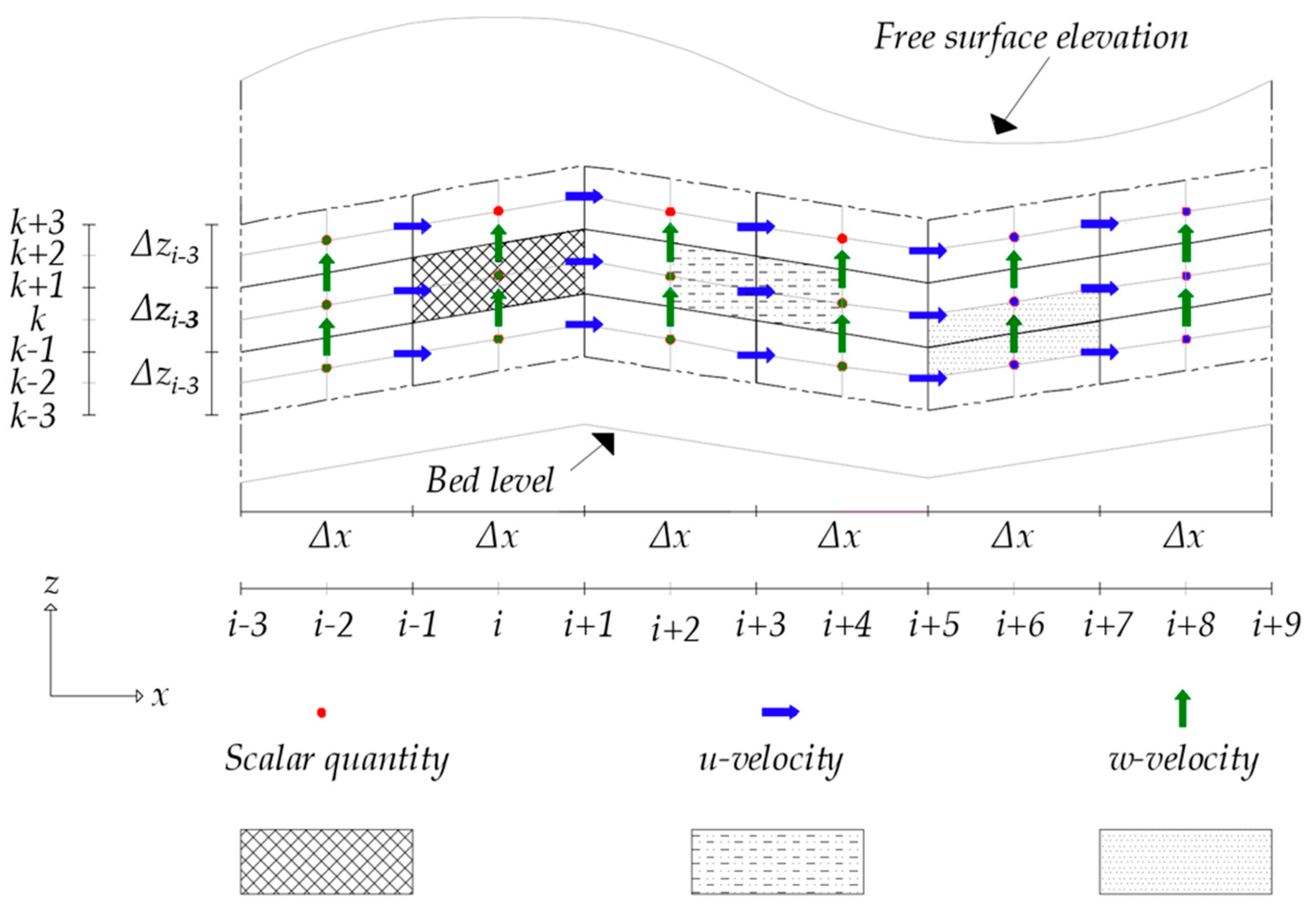
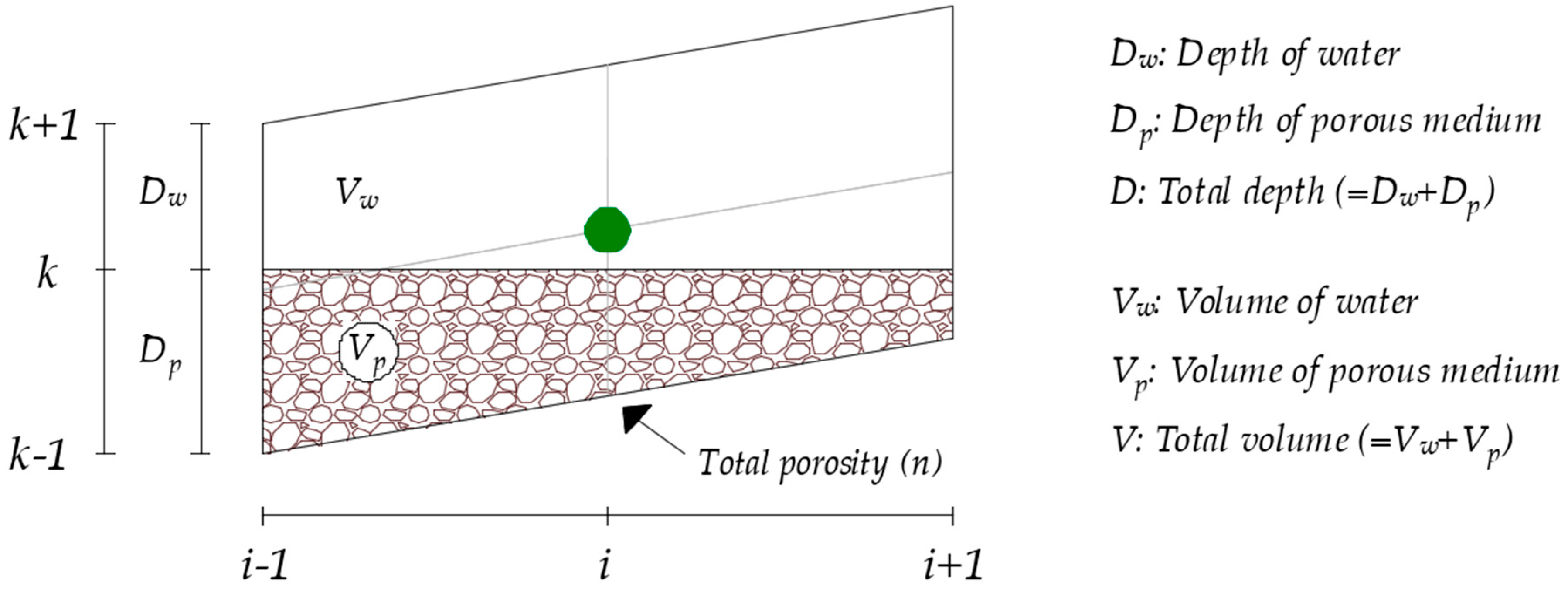
3. Discretization of the Computational Domain

Finite volume method (FVM) in an arbitrary Lagrangian–Eulerian (ALE) system was applied to discretize the governing equations. The arbitrary Lagrangian–Eulerian formulation was developed to combine the advantages of the Lagrangian-based and Eulerian-based formulations, while minimizing their corresponding drawbacks as far as possible. When using the ALE formulation, the nodes on the boundaries and interfaces of the computational mesh can move along with fluid particles in normal Lagrangian fashion to precisely track the boundaries and interfaces, while the nodes of the computational mesh inside the domain can move arbitrarily in a normal Eulerian manner to optimize the shapes of volumes. Because of this freedom in nodes movement was allowed in the ALE formulation, significant distortions of the computational mesh can be reduced in comparison with a purely Lagrangian approach and more resolution can be provided than that allowed by a purely-Eulerian method. Figure 1 illustrates the grid generation system, points of action of scalar and vector quantities, as well as their corresponding control volumes. As shown in Figure 1, scalar variables such as density, pressure, and dynamic viscosity are defined at the center of an individual computational grid, and velocity components are considered at the center of the faces of each control volume. Furthermore, the bed level and free surface elevation in a water column are defined at the center of the lower and the upper side of the control volumes in the base layer and top layer, respectively.

The volume (γ_v) and surface porosity components (γ_x, γ_z) are defined at the center and the faces of each computational grid. A schematic diagram of a partially filled control volume and the definitions of the associated parameters are demonstrated in Figure 2. By considering the temporally varying free surface, the porosity components are updated at each time step by calculating the fraction of each computational grid open to water and the total porosity of porous medium, as follows:

$${\left({\gamma }_v\right)}_{i,k}=\frac{V_W}{V}+n\frac{V_p}{V},$$

(7)

$${\left({\gamma }_x\right)}_{i-1,k}=\frac{D_W}{D}+n\frac{D_p}{D},$$

(8)

It should be noted that for a control volume full of water, the volume and surface porosities are equal to 1 (γ_v = γ_x = γ_z = 1), whereas for a control volume full of porous medium, the porosity components are obtained as total porosity (γ_v = γ_x = γ_z = n).

4. Numerical Implementation

In this study, projection approach suggested by Chorin [27] and Temam [28] was used to solve the extended Navier–Stokes equations in two main steps. In the first fractional step, the pressure fields were excluded from the Navier–Stokes equations and the momentum equations in the absence of pressure gradients were solved to compute an intermediate velocity field (u^*, w^*) that did not satisfy the continuity constraint. The momentum equations in the absence of pressure terms are as follows:

$$\begin{array}{l}{\lambda }_v\frac{u^{*}-u^n}{\Delta t}+\frac{\partial ({\lambda }_x{u}^2)}{\partial x}+\frac{\partial ({\lambda }_{z}uw)}{\partial z}-w_g\frac{\partial ({\gamma }_{x}u)}{\partial z}=\\ \frac{\partial }{\partial x}({\gamma }_x{\upsilon }_T\frac{\partial u}{\partial x})+\frac{\partial }{\partial z}({\gamma }_z{\upsilon }_T\frac{\partial u}{\partial z})-(\frac{\rho }{{\rho }_r})R_x\end{array},$$

(9)

$$\begin{array}{l}{\lambda }_v\frac{w^{*}-w^n}{\Delta t}+\frac{\partial ({\lambda }_{x}wu)}{\partial x}+\frac{\partial ({\lambda }_z{w}^2)}{\partial z}-w_g\frac{\partial ({\gamma }_{z}w)}{\partial z}=\\ \frac{\partial }{\partial x}({\gamma }_x{\upsilon }_T\frac{\partial w}{\partial x})+\frac{\partial }{\partial z}({\gamma }_z{\upsilon }_T\frac{\partial w}{\partial z})-(\frac{\rho }{{\rho }_r})R_z\end{array},$$

(10)

where u^* and w^* are intermediate velocity components, and the superscript n denotes the time level, where $t_n=n.\Delta t$. The terms on the left-hand side of Equations (9) and (10) are advective terms, the first and second terms on the right-hand side of the above equations are diffusive terms, and the third is the drag force component. Therefore, the first step was split into three sub-fractional steps. The first sub-fractional step consists of solving the advective terms and computing the corresponding velocity fields (u^A, w^A) as follows:

$${\lambda }_v\frac{u^A-u^n}{\Delta t}+{\left[\frac{\partial ({\lambda }_x{u}^2)}{\partial x}+\frac{\partial ({\lambda }_{z}uw)}{\partial z}-w_g\frac{\partial ({\gamma }_{x}u)}{\partial z}\right]}^n=0$$

(11)

$${\lambda }_v\frac{w^A-w^n}{\Delta t}+{\left[\frac{\partial ({\lambda }_{x}wu)}{\partial x}+\frac{\partial ({\lambda }_z{w}^2)}{\partial z}-w_g\frac{\partial ({\gamma }_{z}w)}{\partial z}\right]}^n=0,$$

(12)

where the superscript A stands for advection and shows the time level after completing the advection process. It should be noted that Equations (11) and (12) were further split into other three sub-fractional steps. A locally one-dimensional method was applied for solving the above equations and a fifth-order-accurate scheme was utilized to obtain more accurate results for flow characteristics. The second sub-fractional step consists of solving the diffusive terms and calculating the associated velocities (u^D, w^D) as follows:

$${\lambda }_v\frac{u^D-u^A}{\Delta t}=\frac{\partial }{\partial x}\left[{\gamma }_x{\upsilon }_T\frac{\partial }{\partial x}\left((1-{\theta }_D)u^A+{\theta }_D{u}^D\right)\right]+\frac{\partial }{\partial z}\left[{\gamma }_z{\upsilon }_T\frac{\partial }{\partial z}\left((1-{\theta }_D)u^A+{\theta }_D{u}^D\right)\right],$$

(13)

$${\lambda }_v\frac{w^D-w^A}{\Delta t}=\frac{\partial }{\partial x}\left[{\gamma }_x{\upsilon }_T\frac{\partial }{\partial x}\left((1-{\theta }_D)w^A+{\theta }_D{w}^D\right)\right]+\frac{\partial }{\partial z}\left[{\gamma }_z{\upsilon }_T\frac{\partial }{\partial z}\left((1-{\theta }_D)w^A+{\theta }_D{w}^D\right)\right],$$

(14)

where the superscript D stands for diffusion and shows the time level after completing the diffusion process. ${\theta }_D$ is the implicit weighting factor, where ${\theta }_D=1$ denotes a fully implicit approach, whereas ${\theta }_D=0$ implies a fully explicit approach. Equations (13) and (14) were split into other two sub-fractional steps, and the Crank–Nicolson method (${\theta }_D=0.5$) with a central discretization scheme was employed to solve them. The third sub-fractional step consists of solving the drag force components and computing the intermediate velocity fields (u^*, w^*) as follows:

$${\lambda }_v\frac{u^{*}-u^D}{\Delta t}=-{\left(\frac{\rho }{{\rho }_r}\right)}^D{\left(\frac{1}{2}\frac{C_D}{\Delta x}(1-{\gamma }_x)u\sqrt{u^2+w^2}\right)}^D,$$

(15)

$${\lambda }_v\frac{w^{*}-w^D}{\Delta t}=-{\left(\frac{\rho }{{\rho }_r}\right)}^D{\left(\frac{1}{2}\frac{C_D}{\Delta z}(1-{\gamma }_z)w\sqrt{u^2+w^2}\right)}^D,$$

(16)

In the second fractional step, the extended continuity and momentum equations in the absence of advective and diffusive terms and drag force components were solved for the computational cells below the top layer as follows:

$${\left[\frac{\partial ({\gamma }_x{u}^{n+1})}{\partial x}\right]}_{i,k}+{\left[\frac{\partial ({\gamma }_z{w}^{n+1})}{\partial z}\right]}_{i,k}=0,$$

(17)

$${\lambda }_v\frac{u^{n+1}-u^{*}}{\Delta t}=-{\gamma }_v\frac{\partial p^{*}}{\partial x},$$

(18)

$${\lambda }_v\frac{w^{n+1}-w^{*}}{\Delta t}=-{\gamma }_v\frac{\partial p^{*}}{\partial z}-{\gamma }_v\left(\frac{\rho -{\rho }_r}{{\rho }_r}\right)g,$$

(19)

According to the Gauss divergence theorem, Equation (17) can be written as:

$$\begin{array}{l}\frac{1}{A_{i,k}}\left[\begin{array}{l}{\gamma }_x{}_{{}_{i+1,k}}.u_{i+1,k}^{n+1}.(z_{i+1,k+1}-z_{i+1,k-1})+\\ 0.25({\gamma }_x{}_{{}_{i+1,k}}.u_{i+1,k}^{n+1}+{\gamma }_x{}_{{}_{i+1,k+2}}.u_{i+1,k+2}^{n+1}+{\gamma }_x{}_{{}_{i-1,k+2}}.u_{i-1,k+2}^{n+1}+{\gamma }_x{}_{{}_{i-1,k}}.u_{i-1,k}^{n+1}).(z_{i-1,k+1}-z_{i+1,k+1})+\\ {\gamma }_x{}_{{}_{i-1,k}}.u_{i-1,k}^{n+1}.(z_{i-1,k-1}-z_{i-1,k+1})+\\ 0.25({\gamma }_x{}_{{}_{i-1,k}}.u_{i-1,k}^{n+1}+{\gamma }_x{}_{{}_{i-1,k-2}}.u_{i-1,k-2}^{n+1}+{\gamma }_x{}_{{}_{i+1,k-2}}.u_{i+1,k-2}^{n+1}+{\gamma }_x{}_{{}_{i+1,k}}.u_{i+1,k}^{n+1}).(z_{i+1,k-1}-z_{i-1,k-1})\end{array}\right]\\ +\frac{\Delta x}{A_{i,k}}\left[{\gamma }_z{}_{{}_{i,k+1}}.w_{i,k+1}^{n+1}-{\gamma }_z{}_{{}_{i,k-1}}.w_{i,k-1}^{n+1}\right]=0\end{array}$$

(20)

where A_i,k can be calculated as:

$$A_{i,k}=\frac{1}{4}(\Delta z_{i-1}+2\Delta z_i+\Delta z_{i+1})\Delta x,$$

(21)

By considering Equations (18) and (19), the parameters $u_{i\pm 1,k+2}^{n+1}$, $u_{i\pm 1,k}^{n+1}$, $u_{i\pm 1,k-2}^{n+1}$, and $w_{i,k\pm 1}^{n+1}$ can be expressed as follows:

$$u_{i\pm 1,k+2}^{n+1}=u_{i\pm 1,k+2}^{*}-\Delta t\frac{{\gamma }_{v_{i\pm 1,k+2}}}{{\lambda }_{v_{i\pm 1,k+2}}}\left(\phi {\left(\frac{\partial p^{*n+1}}{\partial x}\right)}_{i\pm 1,k+2}+(1-\phi ){\left(\frac{\partial p^{*n}}{\partial x}\right)}_{i\pm 1,k+2}\right),$$

(22)

$$u_{i\pm 1,k}^{n+1}=u_{i\pm 1,k}^{*}-\Delta t\frac{{\gamma }_{v_{i\pm 1,k}}}{{\lambda }_{v_{i\pm 1,k}}}\left(\phi {\left(\frac{\partial p^{*n+1}}{\partial x}\right)}_{i\pm 1,k}+(1-\phi ){\left(\frac{\partial p^{*n}}{\partial x}\right)}_{i\pm 1,k}\right),$$

(23)

$$u_{i\pm 1,k-2}^{n+1}=u_{i\pm 1,k-2}^{*}-\Delta t\frac{{\gamma }_{v_{i\pm 1,k-2}}}{{\lambda }_{v_{i\pm 1,k-2}}}\left(\phi {\left(\frac{\partial p^{*n+1}}{\partial x}\right)}_{i\pm 1,k-2}+(1-\phi ){\left(\frac{\partial p^{*n}}{\partial x}\right)}_{i\pm 1,k-2}\right),$$

(24)

$$w_{i,k\pm 1}^{n+1}=w_{i,k\pm 1}^{*}-\Delta t\frac{{\gamma }_{v_{i,k\pm 1}}}{{\lambda }_{v_{i,k\pm 1}}}\left(\phi {\left(\frac{\partial p^{*n+1}}{\partial z}\right)}_{i,k\pm 1}+(1-\phi ){\left(\frac{\partial p^{*n}}{\partial z}\right)}_{i,k\pm 1}\right)-\Delta t\frac{{\gamma }_{v_{i,k\pm 1}}}{{\lambda }_{v_{i,k\pm 1}}}\left({\left(\frac{\rho }{{\rho }_r}\right)}_{i,k\pm 1}-1\right)g,$$

(25)

Substituting Equations (22)–(25) into Equation (20), the pressure Poisson equation (PPE) can be derived as follows:

$$\begin{array}{l}\frac{1}{A_{i,k}}\left[\begin{array}{l}{\gamma }_x{}_{{}_{i+1,k}}.\left[u_{i+1,k}^{*}-\Delta t\frac{{\gamma }_{v_{i+1,k}}}{{\lambda }_{v_{i+1,k}}}\left(\phi {\left(\frac{\partial p^{*n+1}}{\partial x}\right)}_{i+1,k}+(1-\phi ){\left(\frac{\partial p^{*n}}{\partial x}\right)}_{i+1,k}\right)\right].(z_{i+1,k+1}-z_{i+1,k-1})+\\ 0.25\left(\begin{array}{l}{\gamma }_x{}_{{}_{i+1,k}}.\left[u_{i+1,k}^{*}-\Delta t\frac{{\gamma }_{v_{i+1,k}}}{{\lambda }_{v_{i+1,k}}}\left(\phi {\left(\frac{\partial p^{*n+1}}{\partial x}\right)}_{i+1,k}+(1-\phi ){\left(\frac{\partial p^{*n}}{\partial x}\right)}_{i+1,k}\right)\right]+\\ {\gamma }_x{}_{{}_{i+1,k+2}}.\left[u_{i+1,k+2}^{*}-\Delta t\frac{{\gamma }_{v_{i+1,k+2}}}{{\lambda }_{v_{i+1,k+2}}}\left(\phi {\left(\frac{\partial p^{*n+1}}{\partial x}\right)}_{i+1,k+2}+(1-\phi ){\left(\frac{\partial p^{*n}}{\partial x}\right)}_{i+1,k+2}\right)\right]+\\ {\gamma }_x{}_{{}_{i-1,k+2}}.\left[u_{i-1,k+2}^{*}-\Delta t\frac{{\gamma }_{v_{i-1,k+2}}}{{\lambda }_{v_{i-1,k+2}}}\left(\phi {\left(\frac{\partial p^{*n+1}}{\partial x}\right)}_{i-1,k+2}+(1-\phi ){\left(\frac{\partial p^{*n}}{\partial x}\right)}_{i-1,k+2}\right)\right]+\\ {\gamma }_x{}_{{}_{i-1,k}}.\left[u_{i-1,k}^{*}-\Delta t\frac{{\gamma }_{v_{i-1,k}}}{{\lambda }_{v_{i-1,k}}}\left(\phi {\left(\frac{\partial p^{*n+1}}{\partial x}\right)}_{i-1,k}+(1-\phi ){\left(\frac{\partial p^{*n}}{\partial x}\right)}_{i-1,k}\right)\right]\end{array}\right).(z_{i-1,k+1}-z_{i+1,k+1})+\\ {\gamma }_x{}_{{}_{i-1,k}}.\left[u_{i-1,k}^{*}-\Delta t\frac{{\gamma }_{v_{i-1,k}}}{{\lambda }_{v_{i-1,k}}}\left(\phi {\left(\frac{\partial p^{*n+1}}{\partial x}\right)}_{i-1,k}+(1-\phi ){\left(\frac{\partial p^{*n}}{\partial x}\right)}_{i-1,k}\right)\right].(z_{i-1,k-1}-z_{i-1,k+1})+\\ 0.25\left(\begin{array}{l}{\gamma }_x{}_{{}_{i-1,k}}.\left[u_{i-1,k}^{*}-\Delta t\frac{{\gamma }_{v_{i-1,k}}}{{\lambda }_{v_{i-1,k}}}\left(\phi {\left(\frac{\partial p^{*n+1}}{\partial x}\right)}_{i-1,k}+(1-\phi ){\left(\frac{\partial p^{*n}}{\partial x}\right)}_{i-1,k}\right)\right]+\\ {\gamma }_x{}_{{}_{i-1,k-2}}.\left[u_{i-1,k-2}^{*}-\Delta t\frac{{\gamma }_{v_{i-1,k-2}}}{{\lambda }_{v_{i-1,k-2}}}\left(\phi {\left(\frac{\partial p^{*n+1}}{\partial x}\right)}_{i-1,k-2}+(1-\phi ){\left(\frac{\partial p^{*n}}{\partial x}\right)}_{i-1,k-2}\right)\right]+\\ {\gamma }_x{}_{{}_{i+1,k-2}}.\left[u_{i+1,k-2}^{*}-\Delta t\frac{{\gamma }_{v_{i+1,k-2}}}{{\lambda }_{v_{i+1,k-2}}}\left(\phi {\left(\frac{\partial p^{*n+1}}{\partial x}\right)}_{i+1,k-2}+(1-\phi ){\left(\frac{\partial p^{*n}}{\partial x}\right)}_{i+1,k-2}\right)\right]+\\ {\gamma }_x{}_{{}_{i+1,k}}.\left[u_{i+1,k}^{*}-\Delta t\frac{{\gamma }_{v_{i+1,k}}}{{\lambda }_{v_{i+1,k}}}\left(\phi {\left(\frac{\partial p^{*n+1}}{\partial x}\right)}_{i+1,k}+(1-\phi ){\left(\frac{\partial p^{*n}}{\partial x}\right)}_{i+1,k}\right)\right]\end{array}\right).(z_{i+1,k-1}-z_{i-1,k-1})\end{array}\right]+\\ \frac{\Delta x}{A_{i,k}}\left[\begin{array}{l}{\gamma }_z{}_{{}_{i,k+1}}.\left[w_{i,k+1}^{*}-\Delta t\frac{{\gamma }_{v_{i,k+1}}}{{\lambda }_{v_{i,k+1}}}\left(\phi {\left(\frac{\partial p^{*n+1}}{\partial z}\right)}_{i,k+1}+(1-\phi ){\left(\frac{\partial p^{*n}}{\partial z}\right)}_{i,k+1}\right)-\Delta t\frac{{\gamma }_{v_{i,k+1}}}{{\lambda }_{v_{i,k+1}}}\left({\left(\frac{\rho }{{\rho }_r}\right)}_{i,k+1}-1\right)g\right]-\\ {\gamma }_z{}_{{}_{i,k-1}}.\left[w_{i,k-1}^{*}-\Delta t\frac{{\gamma }_{v_{i,k-1}}}{{\lambda }_{v_{i,k-1}}}\left(\phi {\left(\frac{\partial p^{*n+1}}{\partial z}\right)}_{i,k-1}+(1-\phi ){\left(\frac{\partial p^{*n}}{\partial z}\right)}_{i,k-1}\right)-\Delta t\frac{{\gamma }_{v_{i,k-1}}}{{\lambda }_{v_{i,k-1}}}\left({\left(\frac{\rho }{{\rho }_r}\right)}_{i,k-1}-1\right)g\right]\end{array}\right]=0\end{array}$$

(26)

Using the Gauss divergence theorem for pressure derivatives on the velocity locations, the pressure Poisson equation can be written according to the pressure values in the 15 adjacent cells.

4.1. Pressure Equation at Free Surface Layer

The surface equation is calculated by integrating the extended continuity equation over the depth and considering the kinematic boundary conditions at the impermeable bed level and free surface, as follows:

$$\frac{\partial \xi }{\partial t}-\frac{\partial z_b}{\partial t}+\frac{\partial }{\partial x}{\displaystyle {\int }_{z_b}^{\xi }{\gamma }_{x}udz}=0,$$

(27)

where $\xi$ is defined as the surface elevation above the mean water level and z_b is the impermeable bed level above the datum, which is equal to zero for a fixed bed. The mass continuity equation for the ith water column can be obtained as:

$$\frac{{\xi }_i^{n+1}-{\xi }_i^n}{\Delta t}+\frac{1}{\Delta x}{\displaystyle \sum _{k=k{c}_{\min }}^{k{c}_{\max }}\left[\begin{array}{l}\theta ({\gamma }_x{}_{{}_{i+1,k}}.u_{i+1,k}^{n+1}.\Delta z_{i+1})+(1-\theta )({\gamma }_x{}_{{}_{i+1,k}}.u_{i+1,k}^n.\Delta z_{i+1})\\ -\theta ({\gamma }_x{}_{{}_{i-1,k}}.u_{i-1,k}^{n+1}.\Delta z_{i-1})-(1-\theta )({\gamma }_x{}_{{}_{i-1,k}}.u_{i-1,k}^n.\Delta z_{i-1})\end{array}\right]}=0,$$

(28)

where kc_min and kc_max are the reference numbers of the bottom and the top layers, respectively. The hydrostatic pressure assumption at the top layer may result in inaccurate predictions of the wave phase and water surface elevation. Therefore by applying the non-hydrostatic pressure distribution at the top layer, more accurate results can be obtained for the flow features. In this study, the method proposed by Yuan and Wu was utilized to calculate the pressure equation at free surface layer [29,30]. For the ith water column, the momentum equation in the vertical direction from the center of the top layer to free surface level can be written as follows:

$$\begin{array}{l}{\lambda }_{v_{i,T}}\frac{w_{i,T}^{n+1}-w_{i,T}^{*}}{\Delta t}+{\gamma }_{v_{i,T}}\phi \left(\frac{p_{i,S}^{*n+1}-p_{i,k{c}_{\max }}^{*n+1}}{\frac{1}{8}(\Delta z_{i-1}+2\Delta z_i+\Delta z_{i+1})}\right)+{\gamma }_{v_{i,T}}(1-\phi )\left(\frac{p_{i,S}^{*n}-p_{i,k{c}_{\max }}^{*n}}{\frac{1}{8}(\Delta z_{i-1}+2\Delta z_i+\Delta z_{i+1})}\right)=\\ -{\gamma }_{v_{i,T}}\left({\left(\frac{\rho }{{\rho }_r}\right)}_{i,T}-1\right)g\end{array},$$

(29)

where the subscripts T and S represent the center of the top half-grid and the free surface level, respectively. The parameters $w_{i,T}^{n+1}$ and $w_{i,T}^{*}$ are the vertical velocity components at the distance of 1/4∆z_i from the free surface level and can be approximated by the following equations:

$$w_{i,T}^{n+1}=\frac{3w_{i,k{c}_{\max }+1}^{n+1}+w_{i,k{c}_{\max }-1}^{n+1}}{4},$$

(30)

$$w_{i,T}^{*}=\frac{3w_{i,k{c}_{\max }+1}^{*}+w_{i,k{c}_{\max }-1}^{*}}{4},$$

(31)

In Equation (29), $p_{i,S}^{*n+1}$ and $p_{i,S}^{*n}$ are the pressure at free surface level ($k{c}_{max}+1$) and are calculated as follows:

$$p_{i,S}^{*n+1}={\left(\frac{\rho }{{\rho }_r}\right)}_{i,k{c}_{\max }}g{\xi }_i^{n+1},$$

(32)

$$p_{i,S}^{*n}={\left(\frac{\rho }{{\rho }_r}\right)}_{i,k{c}_{\max }}g{\xi }_i^n,$$

(33)

By substituting Equations (30)–(33) into Equation (29), the momentum equation in the vertical direction and at the top half-grid can be written as follows:

$$\begin{array}{l}{\lambda }_{v_{i,T}}\frac{\left(\frac{3w_{i,k{c}_{\max }+1}^{n+1}+w_{i,k{c}_{\max }-1}^{n+1}}{4}\right)-\left(\frac{3w_{i,k{c}_{\max }+1}^{*}+w_{i,k{c}_{\max }-1}^{*}}{4}\right)}{\Delta t}+{\gamma }_{v_{i,T}}\phi \left(\frac{{\left(\frac{\rho }{{\rho }_r}\right)}_{i,k{c}_{\max }}g{\xi }_i^{n+1}-p_{i,k{c}_{\max }}^{*n+1}}{\frac{1}{8}(\Delta z_{i-1}+2\Delta z_i+\Delta z_{i+1})}\right)+\\ {\gamma }_{v_{i,T}}(1-\phi )\left(\frac{{\left(\frac{\rho }{{\rho }_r}\right)}_{i,k{c}_{\max }}g{\xi }_i^n-p_{i,k{c}_{\max }}^{*n}}{\frac{1}{8}(\Delta z_{i-1}+2\Delta z_i+\Delta z_{i+1})}\right)=-{\gamma }_{v_{i,T}}\left({\left(\frac{\rho }{{\rho }_r}\right)}_{i,T}-1\right)g\end{array},$$

(34)

The volume porosity and density are defined at the center of each grid. Hence, by considering the assumption that ${(\rho /{\rho }_r)}_{i,T}={(\rho /{\rho }_r)}_{i,k{c}_{max }}$, ${\gamma }_{v_{i,T}}={\gamma }_{v_{i,k{c}_{max }}}$, and ${\lambda }_{v_{i,T}}={\lambda }_{v_{i,k{c}_{max }}}$, and by multiplying Equation (34) by 4∆t, the following equation can be obtained:

$$\begin{array}{l}{\lambda }_{v_{i,k{c}_{\max }}}\left(3w_{i,k{c}_{\max }+1}^{n+1}+w_{i,k{c}_{\max }-1}^{n+1}-3w_{i,k{c}_{\max }+1}^{*}-w_{i,k{c}_{\max }-1}^{*}\right)+{\gamma }_{v_{i,k{c}_{\max }}}\frac{32\Delta t}{(\Delta z_{i-1}+2\Delta z_i+\Delta z_{i+1})}\\ \left[\phi \left({\left(\frac{\rho }{{\rho }_r}\right)}_{i,k{c}_{\max }}g{\xi }_i^{n+1}-p_{i,k{c}_{\max }}^{*n+1}\right)+(1-\phi )\left({\left(\frac{\rho }{{\rho }_r}\right)}_{i,k{c}_{\max }}g{\xi }_i^n-p_{i,k{c}_{\max }}^{*n}\right)\right]=\\ -4\Delta t.{\gamma }_{v_{i,k{c}_{\max }}}\left({\left(\frac{\rho }{{\rho }_r}\right)}_{i,k{c}_{\max }}-1\right)g\end{array}$$

(35)

According to Dean and Dalrymple, the kinematic free surface boundary condition is expressed as [31]:

$$w=\frac{\partial \xi }{\partial t}+{\gamma }_{x}u\frac{\partial \xi }{\partial x},$$

(36)

By substituting Equation (27) into Equation (36), the above equation at surface level can be discretized as:

$$\begin{array}{l}{w}_{i,k{c}_{\max }+1}^{n+1}=\left(\frac{{\gamma }_{x_{i-1,k{c}_{\max }}}{u}_{i-1,k{c}_{\max }}^{n+1}+{\gamma }_{x_{i+1,k{c}_{\max }}}{u}_{i+1,k{c}_{\max }}^{n+1}}{2}\right)\left(\frac{{\xi }_{i+2}^n-{\xi }_{i-2}^n}{2\Delta x}\right)-\\ \frac{1}{\Delta x}{\displaystyle \sum _{k=k{c}_{\min }}^{k{c}_{\max }}\left[\begin{array}{l}\theta ({\gamma }_x{}_{{}_{i+1,k}}.u_{i+1,k}^{n+1}.\Delta z_{i+1})+(1-\theta )({\gamma }_x{}_{{}_{i+1,k}}.u_{i+1,k}^n.\Delta z_{i+1})\\ -\theta ({\gamma }_x{}_{{}_{i-1,k}}.u_{i-1,k}^{n+1}.\Delta z_{i-1})-(1-\theta )({\gamma }_x{}_{{}_{i-1,k}}.u_{i-1,k}^n.\Delta z_{i-1})\end{array}\right]}\end{array}$$

(37)

The parameter $w_{i,k{c}_{max}-1}^{n+1}$ can be obtained by writing the momentum equation in the vertical direction, as follows:

$$\begin{array}{l}{w}_{i,k{c}_{\max }-1}^{n+1}=w_{i,k{c}_{\max }-1}^{*}-\Delta t\frac{{\gamma }_{v_{i,k{c}_{\max }-1}}}{{\lambda }_{v_{i,k{c}_{\max }-1}}}\\ \left(\phi \left(\frac{p_{i,k{c}_{\max }}^{*n+1}-p_{i,k{c}_{\max }-2}^{*n+1}}{\frac{1}{4}(\Delta z_{i-1}+2\Delta z_i+\Delta z_{i+1})}\right)+(1-\phi )\left(\frac{p_{i,k{c}_{\max }}^{*n}-p_{i,k{c}_{\max }-2}^{*n}}{\frac{1}{4}(\Delta z_{i-1}+2\Delta z_i+\Delta z_{i+1})}\right)\right)-\\ \Delta t\frac{{\gamma }_{v_{i,k{c}_{\max }-1}}}{{\lambda }_{v_{i,k{c}_{\max }-1}}}\left({\left(\frac{\rho }{{\rho }_r}\right)}_{i,k{c}_{\max }-1}-1\right)g\end{array},$$

(38)

By substituting ${\xi }_i^{n+1}$, $w_{i,k{c}_{max}+1}^{n+1}$, and $w_{i,k{c}_{max}-1}^{n+1}$ from Equations (28), (37), and (38), respectively, Equation (35) can be written as:

$$\begin{array}{l}{\lambda }_{v_{i,k{c}_{\max }}}\left\{\begin{array}{l}3\left[\begin{array}{l}\left(\frac{{\gamma }_{x_{i-1,k{c}_{\max }}}{u}_{i-1,k{c}_{\max }}^{n+1}+{\gamma }_{x_{i+1,k{c}_{\max }}}{u}_{i+1,k{c}_{\max }}^{n+1}}{2}\right)\left(\frac{{\xi }_{i+2}^n-{\xi }_{i-2}^n}{2\Delta x}\right)-\\ \frac{1}{\Delta x}{\displaystyle \sum _{k=k{c}_{\min }}^{k{c}_{\max }}\left[\begin{array}{l}{\theta }^{\prime }({\gamma }_x{}_{{}_{i+1,k}}.u_{i+1,k}^{n+1}.\Delta z_{i+1})+(1-{\theta }^{\prime })({\gamma }_x{}_{{}_{i+1,k}}.u_{i+1,k}^n.\Delta z_{i+1})\\ -{\theta }^{\prime }({\gamma }_x{}_{{}_{i-1,k}}.u_{i-1,k}^{n+1}.\Delta z_{i-1})-(1-{\theta }^{\prime })({\gamma }_x{}_{{}_{i-1,k}}.u_{i-1,k}^n.\Delta z_{i-1})\end{array}\right]}\end{array}\right]+\\ \left[\begin{array}{l}{w}_{i,k{c}_{\max }-1}^{*}-\\ \Delta t\frac{{\gamma }_{v_{i,k{c}_{\max }-1}}}{{\lambda }_{v_{i,k{c}_{\max }-1}}}\left(\phi \left(\frac{p_{i,k{c}_{\max }}^{*n+1}-p_{i,k{c}_{\max }-2}^{*n+1}}{\frac{1}{4}(\Delta z_{i-1}+2\Delta z_i+\Delta z_{i+1})}\right)+(1-\phi )\left(\frac{p_{i,k{c}_{\max }}^{*n}-p_{i,k{c}_{\max }-2}^{*n}}{\frac{1}{4}(\Delta z_{i-1}+2\Delta z_i+\Delta z_{i+1})}\right)\right)-\\ \Delta t\frac{{\gamma }_{v_{i,k{c}_{\max }-1}}}{{\lambda }_{v_{i,k{c}_{\max }-1}}}\left({\left(\frac{\rho }{{\rho }_r}\right)}_{i,k{c}_{\max }-1}-1\right)g\end{array}\right]-3w_{i,k{c}_{\max }+1}^{*}-w_{i,k{c}_{\max }-1}^{*}\end{array}\right\}+\\ {\gamma }_{v_{i,k{c}_{\max }}}\frac{32\Delta t}{(\Delta z_{i-1}+2\Delta z_i+\Delta z_{i+1})}\\ \left[\begin{array}{l}\phi \left({\left(\frac{\rho }{{\rho }_r}\right)}_{i,k{c}_{\max }}g\left\{{\xi }_i^n-\frac{\Delta t}{\Delta x}{\displaystyle \sum _{k=k{c}_{\min }}^{k{c}_{\max }}\left[\begin{array}{l}\theta ({\gamma }_x{}_{{}_{i+1,k}}.u_{i+1,k}^{n+1}.\Delta z_{i+1})+(1-\theta )({\gamma }_x{}_{{}_{i+1,k}}.u_{i+1,k}^n.\Delta z_{i+1})\\ -\theta ({\gamma }_x{}_{{}_{i-1,k}}.u_{i-1,k}^{n+1}.\Delta z_{i-1})-(1-\theta )({\gamma }_x{}_{{}_{i-1,k}}.u_{i-1,k}^n.\Delta z_{i-1})\end{array}\right]}\right\}-p_{i,k{c}_{\max }}^{*n+1}\right)+\\ (1-\phi )\left({\left(\frac{\rho }{{\rho }_r}\right)}_{i,k{c}_{\max }}g{\xi }_i^n-p_{i,k{c}_{\max }}^{*n}\right)\end{array}\right]=\\ -4\Delta t.{\gamma }_{v_{i,k{c}_{\max }}}\left({\left(\frac{\rho }{{\rho }_r}\right)}_{i,k{c}_{\max }}-1\right)g\end{array}$$

(39)

By substituting horizontal velocity components from Equation (23) into Equation (39), the pressure equation at surface layer is obtained as:

$$\begin{array}{l}\hspace{0.17em}{\lambda }_{v_{i,k{c}_{\max }}}\left\{\begin{array}{l}3\left[\begin{array}{l}\frac{1}{2}\left[\begin{array}{l}{\gamma }_{x_{i-1,k{c}_{\max }}}\left[u_{i-1,k{c}_{\max }}^{*}-\Delta t\frac{{\gamma }_{v_{i-1,k{c}_{\max }}}}{{\lambda }_{v_{i-1,k{c}_{\max }}}}\left(\phi {\left(\frac{\partial p^{*n+1}}{\partial x}\right)}_{i-1,k{c}_{\max }}+(1-\phi ){\left(\frac{\partial p^{*n}}{\partial x}\right)}_{i-1,k{c}_{\max }}\right)\right]+\\ {\gamma }_{x_{i+1,k{c}_{\max }}}\left[u_{i+1,k{c}_{\max }}^{*}-\Delta t\frac{{\gamma }_{v_{i+1,k{c}_{\max }}}}{{\lambda }_{v_{i+1,k{c}_{\max }}}}\left(\phi {\left(\frac{\partial p^{*n+1}}{\partial x}\right)}_{i+1,k{c}_{\max }}+(1-\phi ){\left(\frac{\partial p^{*n}}{\partial x}\right)}_{i+1,k{c}_{\max }}\right)\right]\end{array}\right].\left(\frac{{\xi }_{i+2}^n-{\xi }_{i-2}^n}{2\Delta x}\right)-\\ \frac{1}{\Delta x}{\displaystyle \sum _{k=k{c}_{\min }}^{k{c}_{\max }}\left[\begin{array}{l}{\theta }^{\prime }\left({\gamma }_x{}_{{}_{i+1,k}}.\left[u_{i+1,k}^{*}-\Delta t\frac{{\gamma }_{v_{i+1,k}}}{{\lambda }_{v_{i+1,k}}}\left(\phi {\left(\frac{\partial p^{*n+1}}{\partial x}\right)}_{i+1,k}+(1-\phi ){\left(\frac{\partial p^{*n}}{\partial x}\right)}_{i+1,k}\right)\right].\Delta z_{i+1}\right)+\\ (1-{\theta }^{\prime })({\gamma }_x{}_{{}_{i+1,k}}.u_{i+1,k}^n.\Delta z_{i+1})-\\ {\theta }^{\prime }\left({\gamma }_x{}_{{}_{i-1,k}}.\left[u_{i-1,k}^{*}-\Delta t\frac{{\gamma }_{v_{i-1,k}}}{{\lambda }_{v_{i-1,k}}}\left(\phi {\left(\frac{\partial p^{*n+1}}{\partial x}\right)}_{i-1,k}+(1-\phi ){\left(\frac{\partial p^{*n}}{\partial x}\right)}_{i-1,k}\right)\right].\Delta z_{i-1}\right)-\\ (1-{\theta }^{\prime })({\gamma }_x{}_{{}_{i-1,k}}.u_{i-1,k}^n.\Delta z_{i-1})\end{array}\right]}\end{array}\right]+\\ \left[\begin{array}{l}-\frac{4\Delta t}{(\Delta z_{i-1}+2\Delta z_i+\Delta z_{i+1})}\frac{{\gamma }_{v_{i,k{c}_{\max }-1}}}{{\lambda }_{v_{i,k{c}_{\max }-1}}}\left(\phi \left(p_{i,k{c}_{\max }}^{*n+1}-p_{i,k{c}_{\max }-2}^{*n+1}\right)+(1-\phi )\left(p_{i,k{c}_{\max }}^{*n}-p_{i,k{c}_{\max }-2}^{*n}\right)\right)-\\ \Delta t\frac{{\gamma }_{v_{i,k{c}_{\max }-1}}}{{\lambda }_{v_{i,k{c}_{\max }-1}}}\left({\left(\frac{\rho }{{\rho }_r}\right)}_{i,k{c}_{\max }-1}-1\right)g\end{array}\right]-3w_{i,k{c}_{\max }+1}^{*}\end{array}\right\}+\\ {\gamma }_{v_{i,k{c}_{\max }}}\frac{32\Delta t}{(\Delta z_{i-1}+2\Delta z_i+\Delta z_{i+1})}\\ \left[\begin{array}{l}\phi \left({\left(\frac{\rho }{{\rho }_r}\right)}_{i,k{c}_{\max }}g\left\{{\xi }_i^n-\frac{\Delta t}{\Delta x}{\displaystyle \sum _{k=k{c}_{\min }}^{k{c}_{\max }}\left[\begin{array}{l}\theta \left({\gamma }_x{}_{{}_{i+1,k}}.\left[u_{i+1,k}^{*}-\Delta t\frac{{\gamma }_{v_{i+1,k}}}{{\lambda }_{v_{i+1,k}}}\left(\phi {\left(\frac{\partial p^{*n+1}}{\partial x}\right)}_{i+1,k}+(1-\phi ){\left(\frac{\partial p^{*n}}{\partial x}\right)}_{i+1,k}\right)\right].\Delta z_{i+1}\right)+\\ (1-\theta )\left({\gamma }_x{}_{{}_{i+1,k}}.u_{i+1,k}^n.\Delta z_{i+1}\right)-\\ \theta \left({\gamma }_x{}_{{}_{i-1,k}}.\left[u_{i-1,k}^{*}-\Delta t\frac{{\gamma }_{v_{i-1,k}}}{{\lambda }_{v_{i-1,k}}}\left(\phi {\left(\frac{\partial p^{*n+1}}{\partial x}\right)}_{i-1,k}+(1-\phi ){\left(\frac{\partial p^{*n}}{\partial x}\right)}_{i-1,k}\right)\right].\Delta z_{i-1}\right)-\\ (1-\theta )({\gamma }_x{}_{{}_{i-1,k}}.u_{i-1,k}^n.\Delta z_{i-1})\end{array}\right]}\right\}-p_{i,k{c}_{\max }}^{*n+1}\right)+\\ (1-\phi )\left({\left(\frac{\rho }{{\rho }_r}\right)}_{i,k{c}_{\max }}g{\xi }_i^n-p_{i,k{c}_{\max }}^{*n}\right)\end{array}\right]=\\ -4\Delta t.{\gamma }_{v_{i,k{c}_{\max }}}\left({\left(\frac{\rho }{{\rho }_r}\right)}_{i,k{c}_{\max }}-1\right)g\end{array}$$

(40)

By applying the finite difference method (FDM) for discretization of pressure derivatives at the top layer and gauss divergence theorem for pressure derivatives below the top layer, the pressure equation at the free surface layer can be obtained according to the pressure values at ith column and two adjacent water columns.

4.2. Numerical Solution of the Pressure Poisson Equation (PPE)

By applying Equation (40) for cells that are located at the top layer of the numerical domain and pressure Poisson Equation (26) for cells below the top layer, the system of partial differential equations (PDEs) is written as follows:

$$\overline{\overline{A}}{\overline{p}}^{*}{}_{ic-2}^{n+1}+\overline{\overline{B}}{\overline{p}}^{*}{}_{ic}^{n+1}+\overline{\overline{C}}{\overline{p}}^{*}{}_{ic+2}^{n+1}={\overline{D}}_i,$$

(41)

where ic is the reference number of the center of computational grids in the x direction. The above equation can be rewritten as follows:

$$\left[\begin{array}{ccccccccc}{B}_{ic}{}_{{}_{\min }}& C_{ic}{}_{{}_{\min }}& & & & .& .& .& 0\\ A_{ic}{}_{{}_{\min +2}}& B_{ic}{}_{{}_{\min +2}}& C_{ic}{}_{{}_{\min +2}}& & & & & & .\\ & .& .& .& & & & & .\\ & & .& .& .& & & & .\\ & & & A_{ic}& B_{ic}& C_{ic}& & & \\ .& & & & .& .& .& & \\ .& & & & & .& .& .& \\ .& & & & & & A_{ic}{}_{{}_{\max -2}}& B_{ic}{}_{{}_{\max -2}}& C_{ic}{}_{{}_{\max -2}}\\ 0& .& .& .& & & & A_{ic}{}_{{}_{\max }}& B_{ic}{}_{{}_{\max }}\end{array}\right].\left[\begin{array}{c}{p}^{*}{}_{i{c}_{\min }}^{n+1}\\ p^{*}{}_{i{c}_{\min +2}}^{n+1}\\ .\\ .\\ p^{*}{}_{ic}^{n+1}\\ .\\ .\\ p^{*}{}_{i{c}_{\max -2}}^{n+1}\\ p^{*}{}_{i{c}_{\max }}^{n+1}\end{array}\right]=\left[\begin{array}{c}{D}_{ic}{}_{{}_{\min }}\\ D_{ic}{}_{{}_{\min +2}}\\ .\\ .\\ D_{ic}\\ .\\ .\\ D_{ic}{}_{{}_{\max -2}}\\ D_{ic}{}_{{}_{\max }}\end{array}\right],$$

(42)

where $p_{ic}^{*n+1}$ is the unknown pressure vector at icth column and is expressed as:

$$p^{*}{}_{ic}^{n+1}=\left[p^{*}{}_{ic,k{c}_{\min }}^{n+1},p^{*}{}_{ic,k{c}_{\min }+2}^{n+1},\dots ,p^{*}{}_{ic,kc}^{n+1},\dots ,p^{*}{}_{ic,k{c}_{\max -2}}^{n+1},p^{*}{}_{ic,k{c}_{\max }}^{n+1}\right],$$

(43)

The coefficient matrix in Equation (42) forms a block tri-diagonal matrix, which has the dimension of $\left[1/2\left(i{c}_{{}_{\max }}-i{c}_{{}_{\min }}\right)+1\right]\times \left[1/2\left(i{c}_{{}_{\max }}-i{c}_{{}_{\min }}\right)+1\right]$, and each block takes the following form:

$$\left[\begin{array}{ccccccccccc}{f}_{k{c}_{\min }}{}_{{}_{k{c}_{\min }}}& f_{k{c}_{\min }}{}_{{}_{k{c}_{\min +2}}}& f_{k{c}_{\min }}{}_{{}_{k{c}_{\min +4}}}& & & & & .& .& .& 0\\ f_{k{c}_{\min +2}}{}_{{}_{k{c}_{\min }}}& f_{k{c}_{\min +2}}{}_{{}_{k{c}_{\min +2}}}& f_{k{c}_{\min +2}}{}_{{}_{k{c}_{\min +4}}}& f_{k{c}_{\min +2}}{}_{{}_{k{c}_{\min +6}}}& & & & & & & .\\ f_{k{c}_{\min +4}}{}_{{}_{k{c}_{\min }}}& f_{k{c}_{\min +4}}{}_{{}_{k{c}_{\min }+2}}& f_{k{c}_{\min +4}}{}_{{}_{k{c}_{\min +4}}}& f_{k{c}_{\min +4}}{}_{{}_{k{c}_{\min +6}}}& f_{k{c}_{\min +4}}{}_{{}_{k{c}_{\min }+8}}& & & & & & .\\ & .& .& .& .& .& & & & & .\\ & & .& .& .& .& .& & & & \\ & & & f_{kc}{}_{{}_{kc-4}}& f_{kc}{}_{{}_{kc-2}}& f_{kc}{}_{{}_{kc}}& f_{kc}{}_{{}_{kc+2}}& f_{kc}{}_{{}_{kc+4}}& & & \\ .& & & & .& .& .& .& .& & \\ .& & & & & .& .& .& .& .& \\ .& & & & & & f_{k{c}_{\max -4}}{}_{{}_{k{c}_{\max -8}}}& f_{k{c}_{\max -4}}{}_{{}_{k{c}_{\max -6}}}& f_{k{c}_{\max -4}}{}_{{}_{k{c}_{\max -4}}}& f_{k{c}_{\max -4}}{}_{{}_{k{c}_{\max -2}}}& f_{k{c}_{\max -4}}{}_{{}_{k{c}_{\max }}}\\ 0& .& .& .& & & & f_{k{c}_{\max -2}}{}_{{}_{k{c}_{\max -6}}}& f_{k{c}_{\max -2}}{}_{{}_{k{c}_{\max -4}}}& f_{k{c}_{\max -2}}{}_{{}_{k{c}_{\max -2}}}& f_{k{c}_{\max -2}}{}_{{}_{k{c}_{\max }}}\\ f_{k{c}_{\max }}{}_{{}_{k{c}_{\min }}}& f_{k{c}_{\max }}{}_{{}_{k{c}_{\min +2}}}& .& .& .& f_{k{c}_{\max }}{}_{{}_{kc}}& .& .& .& f_{k{c}_{\max }}{}_{{}_{k{c}_{\max -2}}}& f_{k{c}_{\max }}{}_{{}_{k{c}_{\max }}}\end{array}\right]$$

(44)

with the exception of top layer, it is a five-diagonal matrix with the dimension of $\left[1/2\left(k{c}_{{}_{\max }}-k{c}_{{}_{\min }}\right)+1\right]\times \left[1/2\left(k{c}_{{}_{\max }}-k{c}_{{}_{\min }}\right)+1\right]$.

In the presented model, the system of partial differential equations (Equation (42)) was solved by applying a direct approach of the Thomas algorithm, and pressure fields were calculated for the whole computational domain. After calculating the pressure fields, the velocity components at the new time level (uⁿ⁺¹, wⁿ⁺¹) were obtained by solving Equations (18) and (19). Then, the free surface elevation was updated by using Equation (28) and the new grid system was generated to fit the new surface level and to initiate the next time step.

4.3. Initial Boundary Conditions

Two types of boundary conditions, namely, Dirichlet and Neumann were used in the present model. The Dirichlet boundary condition assumed zero for vertical velocity components at impermeable bed, and the Neumann boundary condition was imposed by assuming zero for normal gradient of the horizontal velocity components at impermeable bed and the vertical velocity components at the left side of the numerical domain. Furthermore, horizontal velocity components at the upstream boundary were specified as inflow conditions at x = 0. A free exit for the flow was considered at the downstream boundary of the domain by considering the dynamic pressure equal to zero.

5. Results and Discussions

Before proceeding to the study of wave interaction with a permeable coastal structure, the accuracy of the model in the absence of the porous medium must be evaluated. In this regard, the numerical model is firstly validated by comparing the numerical predictions with the analytical solutions proposed for the determination of the Stokes and solitary wave propagation in a wave tank. It can be derived from Equations (7) and (8)—for a control volume full of water the porosity components are equal to 1 (γ_v $=$ γ_x $=$ γ_z $=$ 1) and the governing extended Navier–Stokes equations become identical to the conventional equations. This implementation was considered in the two following sections. Then, the model was utilized to investigate the solitary wave interaction with a permeable submerged breakwater and the model results were compared with the experimental measurements.

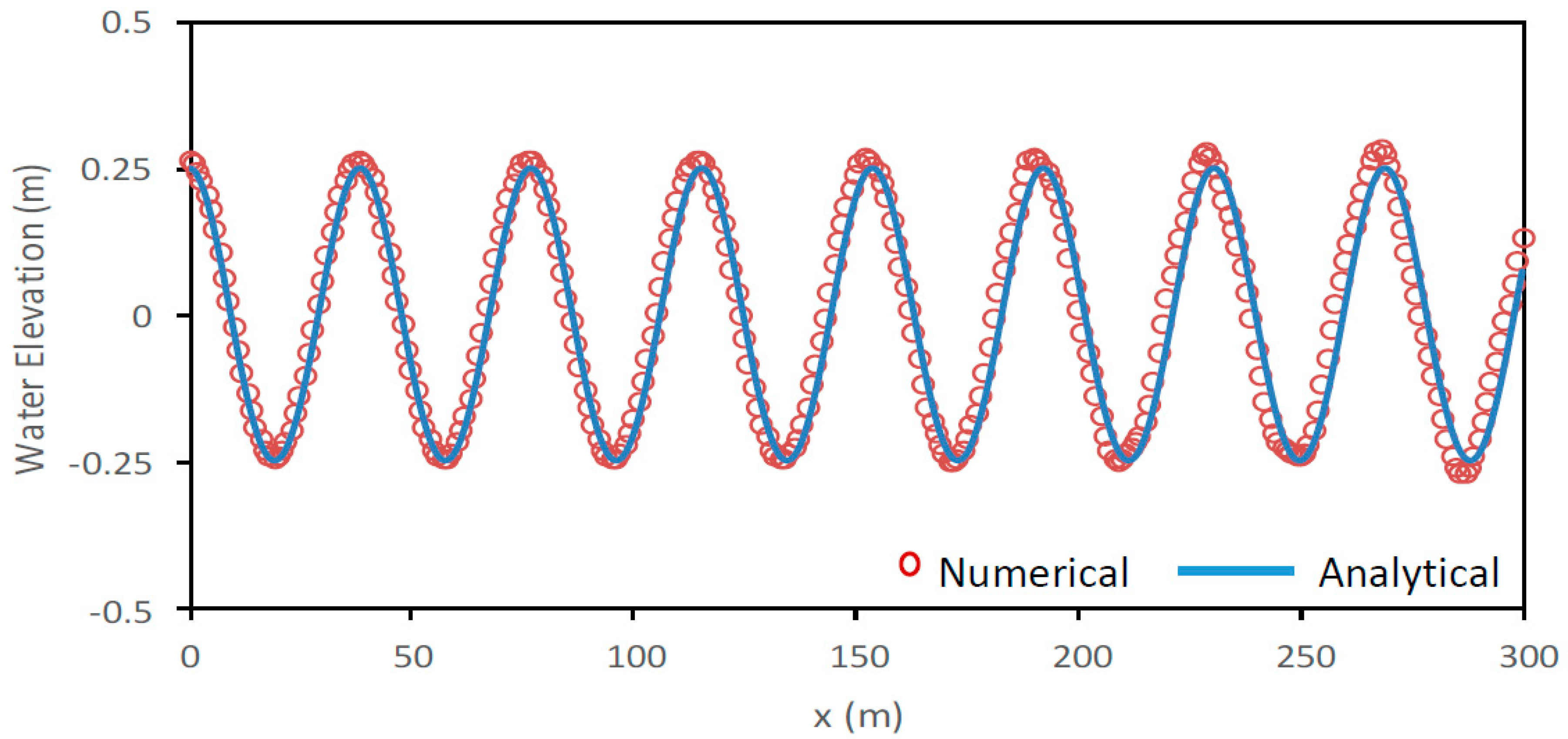
5.1. Progressive Stokes Waves Propagation

The capability of the newly developed model for simulating the non-linear progressive wave train in a deep water was firstly evaluated. An incident wave with the height of $H=0.5 \mathrm{m}$ and wave period of $T=5 \mathrm{s}$ propagated in a water depth of $h=15 \mathrm{m}$. According to the validity range of various wave theories presented by Le Méhauté [32], the second-order Stokes wave was obtained for the above features. For second-order Stokes waves, the linear dispersion Equation (45) is valid [33]; therefore, the wave number can be obtained as $k=0.16344 \mathrm{rad}/\mathrm{m}$.

$${\sigma }^2=gk.\tanh kh,$$

(45)

Using equations $k=2\pi /L$ and $C=L/T$, the wave length and wave celerity are calculated as $38.44 \mathrm{m}$ and

, respectively. The numerical domain with a length of $L=1500 \mathrm{m}$ was discretized with uniform grids of $\Delta x=1 \mathrm{m}$ in the horizontal direction and $15$ layers in the vertical direction. The increment of dimensionless time was chosen to be $\Delta t=0.05 \mathrm{s}$ and a total simulation time of $t=140 \mathrm{s}$ was adopted. For second-order Stokes waves, the analytical equations for surface elevation and velocity components are obtained by [34]:

$$\eta =\frac{H}{2}\cos \left(kx-\sigma t\right)+\frac{H^{2}k}{16}\frac{\cosh kh}{{\sinh }^{3}kh}(2+\cosh 2kh).\cos 2(kx-\sigma t),$$

(46)

$$u=\frac{Hgk}{2\sigma }\frac{\cosh kz}{\cosh kh}\cos (kx-\sigma t)+\frac{3H^2\sigma k}{16}\frac{\cosh 2kz}{{\sinh }^{4}kh}\cos 2(kx-\sigma t),$$

(47)

$$w=\frac{Hgk}{2\sigma }\frac{\sinh kz}{\cosh kh}\sin (kx-\sigma t)+\frac{3H^2\sigma k}{16}\frac{\sinh 2kz}{{\sinh }^{4}kh}\sin 2(kx-\sigma t),$$

(48)

where $z$ is the elevation above the datum and $\sigma =2\pi /T$ is the angular frequency. Comparison between numerical result and analytical solution for free surface displacements at $t=140 \mathrm{s}$, is shown in Figure 3.

As shown in Figure 3, the predicted results agree well with analytical solution for free surface evolution.

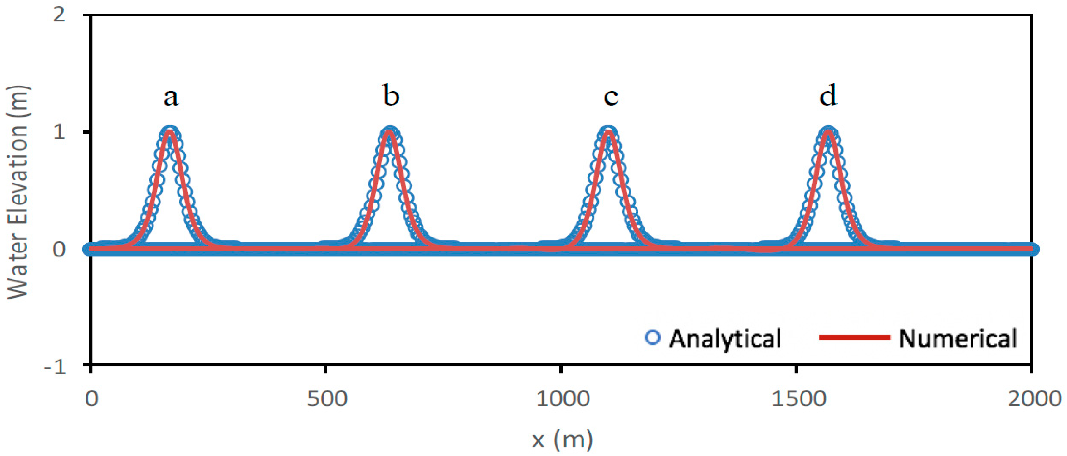
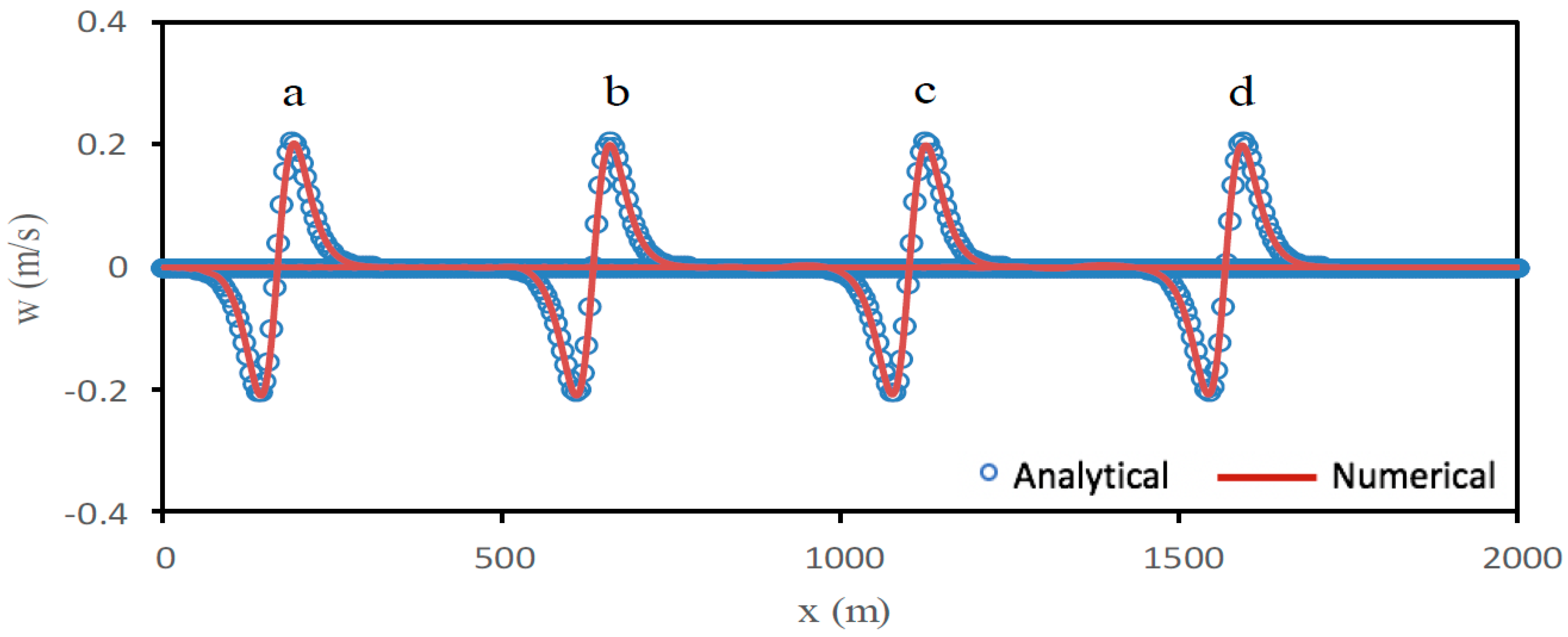
5.2. Solitary Wave Propagation

A numerical wave tank with the length of $L=2000 \mathrm{m}$ was used and a solitary wave with the amplitude of $H=1 \mathrm{m}$ propagated in a constant water depth of $h=10 \mathrm{m}$. A uniform grid system with $\Delta x=2 \mathrm{m}$ in the $x$ direction and $10$ layers in the $z$ direction was deployed for the discretization of the computational domain. The numerical time interval was set at $\Delta t=0.1 \mathrm{s}$, and calculations were continued for $t=180 \mathrm{s}$. According to Boussinesq equations, the analytical free surface displacements and velocity components are derived as proposed by Lee et al. [33]:

$$\eta =H{\mathrm{sech}}^2\left(\sqrt{\frac{3}{4}\frac{H}{h^3}}X\right); X=(x-ct)$$

(49)

$$u=\sqrt{gh}\frac{\eta }{h}\left[1-\frac{1}{4}\frac{\eta }{h}+\frac{h}{3}\frac{h}{\eta }\left(1-\frac{3}{2}\frac{z^2}{h^2}\right)\frac{d^2\eta }{dX{}_2}\right]$$

(50)

$$w=-\sqrt{gh}\frac{z}{h}\left[\left(1-\frac{1}{2}\frac{\eta }{h}\right)\frac{d\eta }{dX}+\frac{1}{3}{h}^2\left(1-\frac{1}{2}\frac{z^2}{h^2}\right)\frac{d^3\eta }{dX{}_3}\right]$$

(51)

where $c=\sqrt{g\left(h+H\right)}$ is the celerity of the solitary wave which can be obtained as $c=10.388 \mathrm{m}/\mathrm{s}$. By assuming the upstream inflow boundary at $x=-300 \mathrm{m}$, the solitary wave in the computational domain will start at its highest point. Figure 4, Figure 5 and Figure 6 compare the numerical predictions and analytical solutions for the surface evolution and velocity components in the x and z directions, respectively.

The figures show that the newly developed model provides a high accuracy level in predicting the free surface distribution and velocity components.

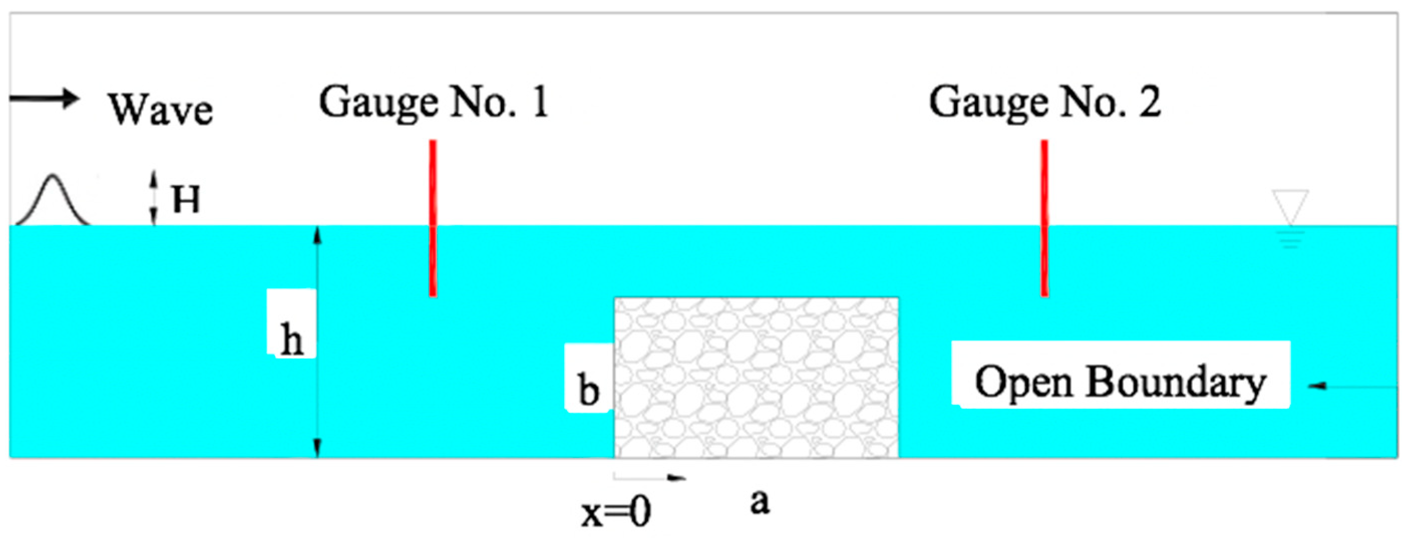
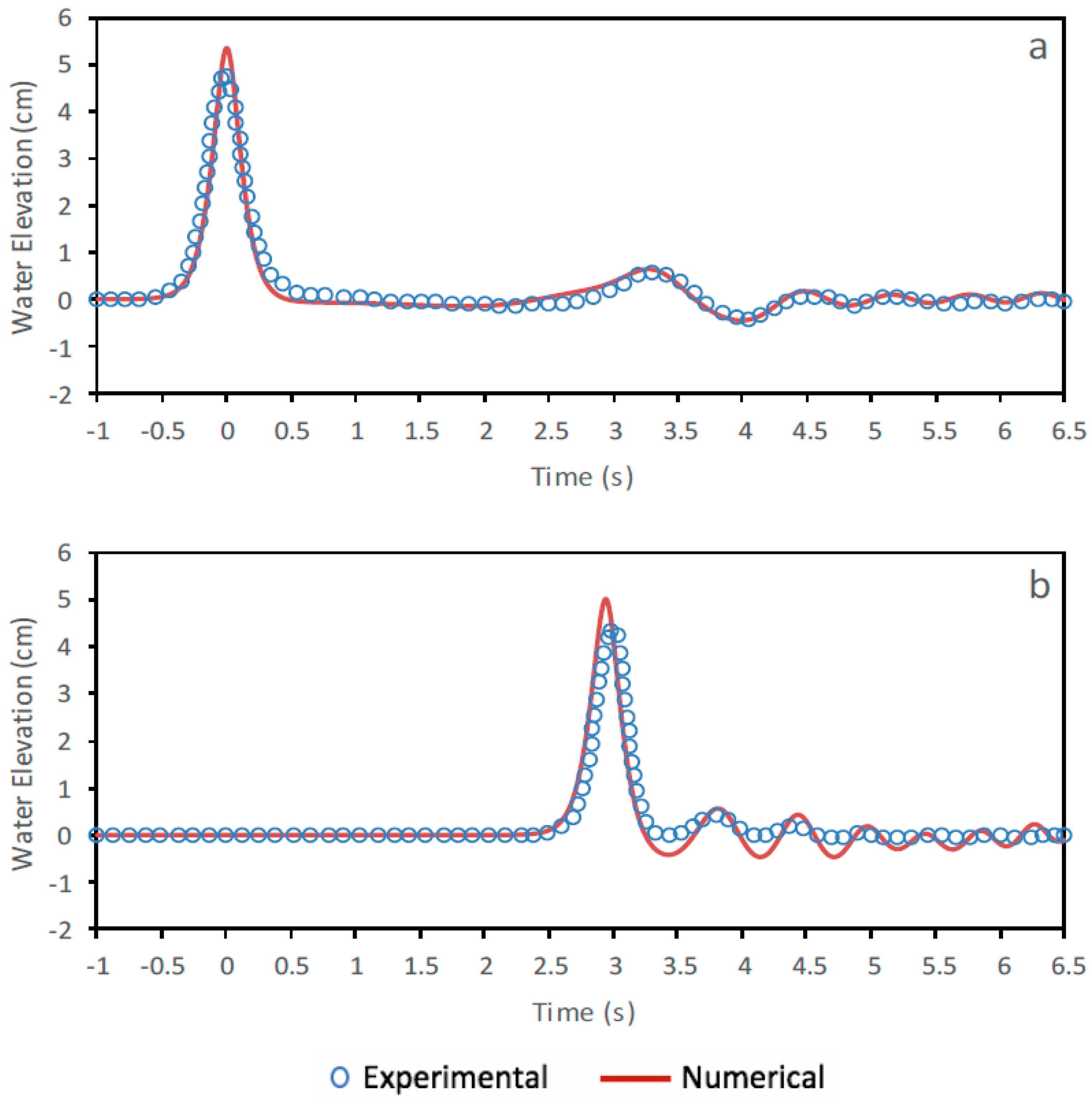
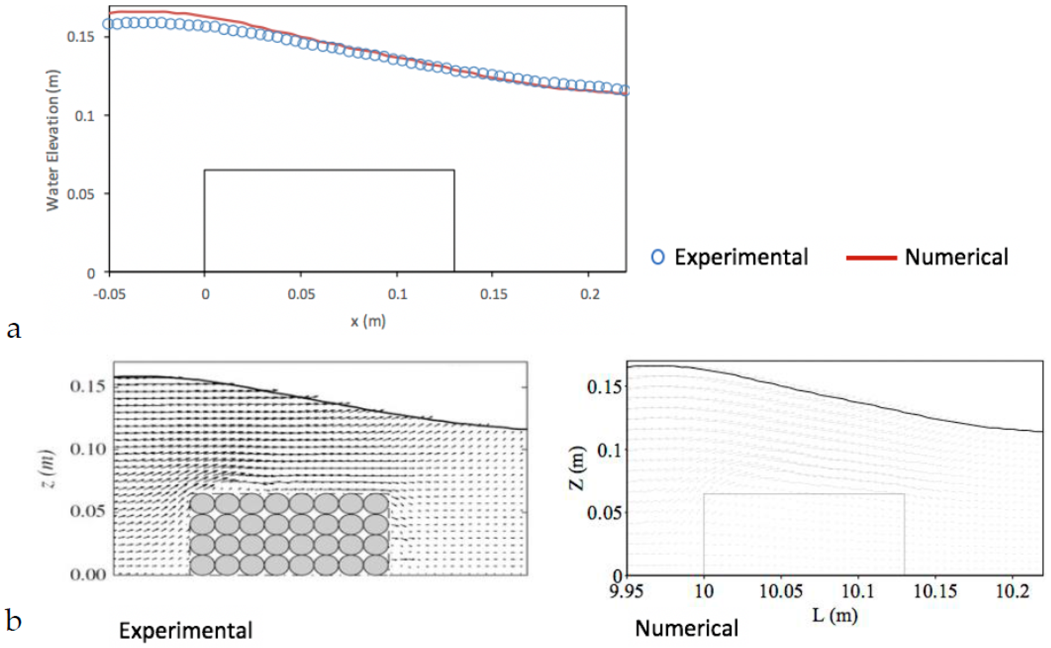
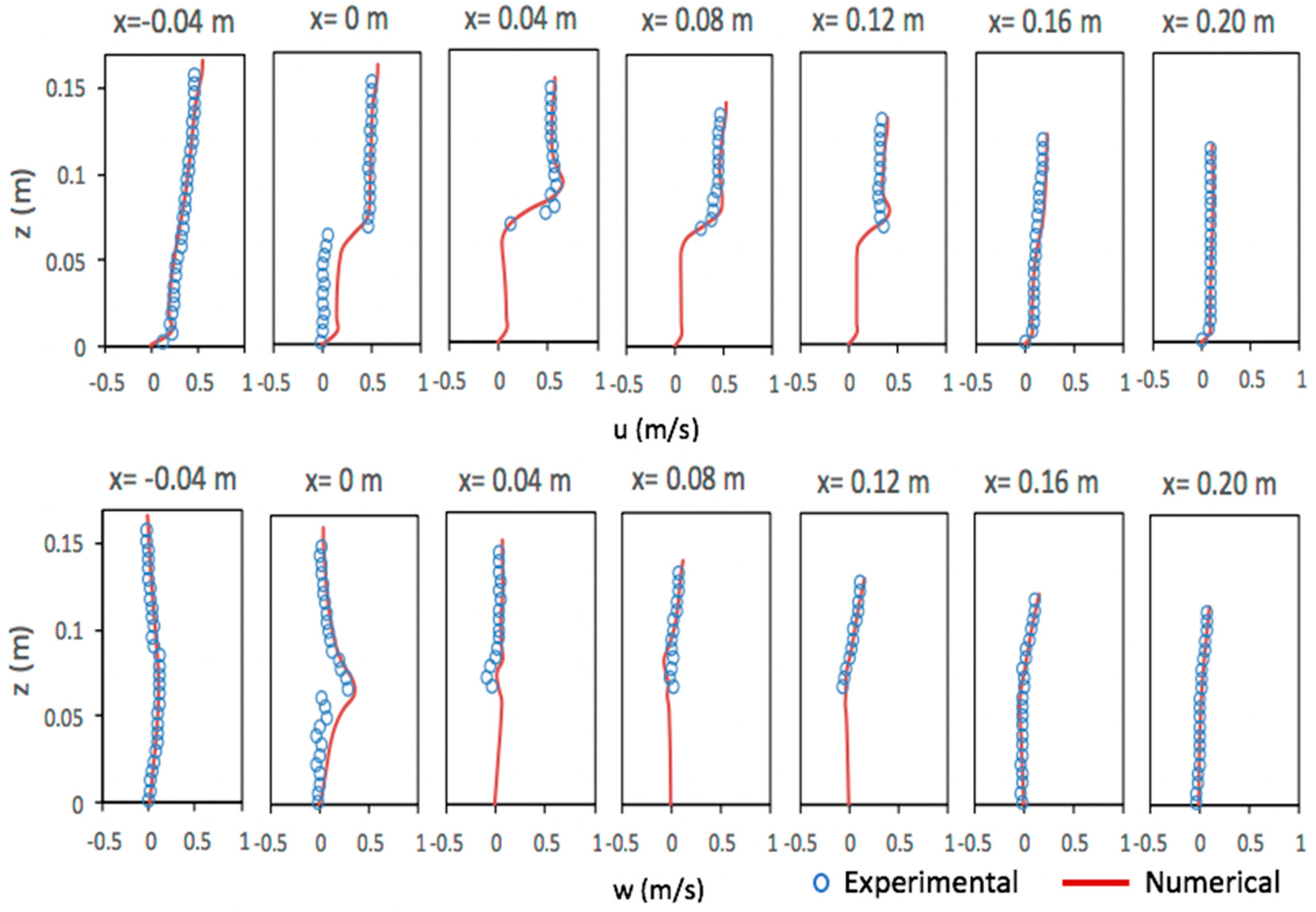
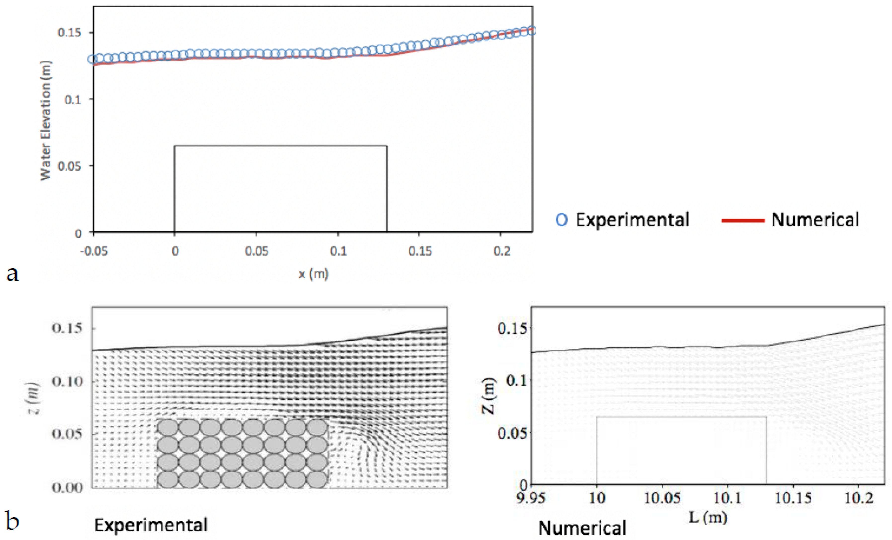
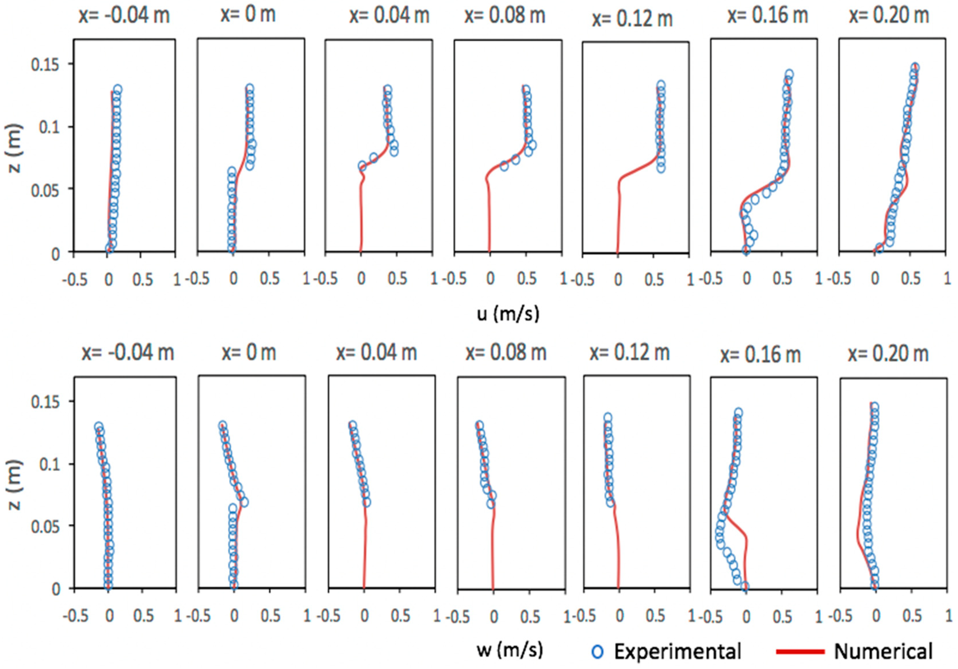
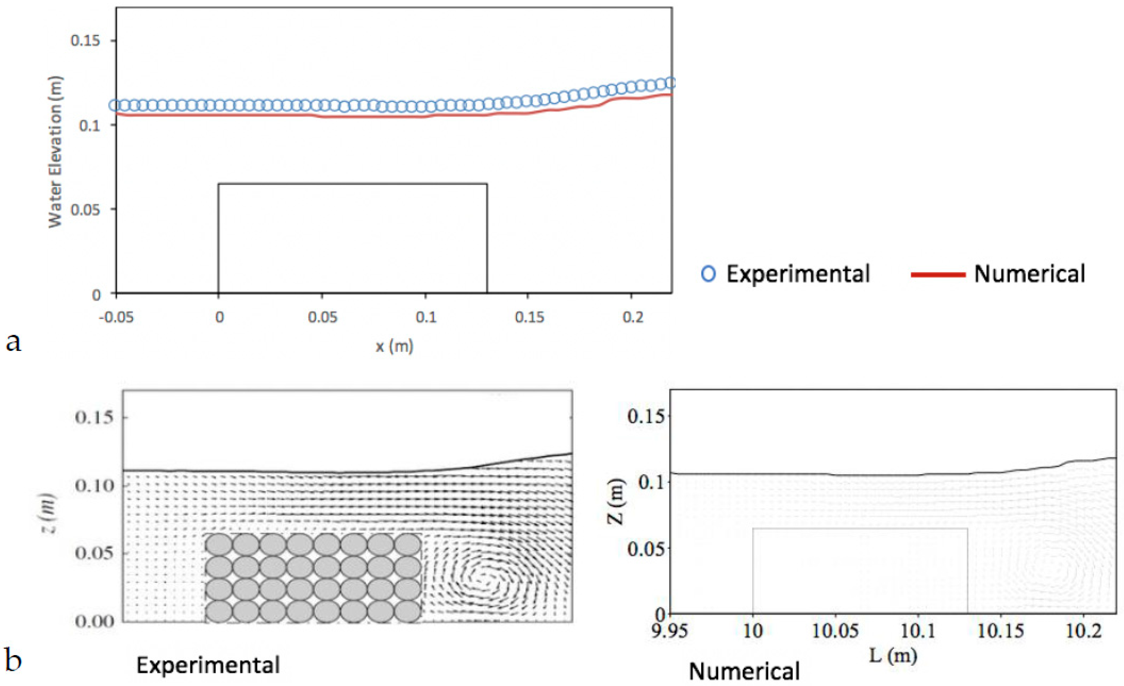
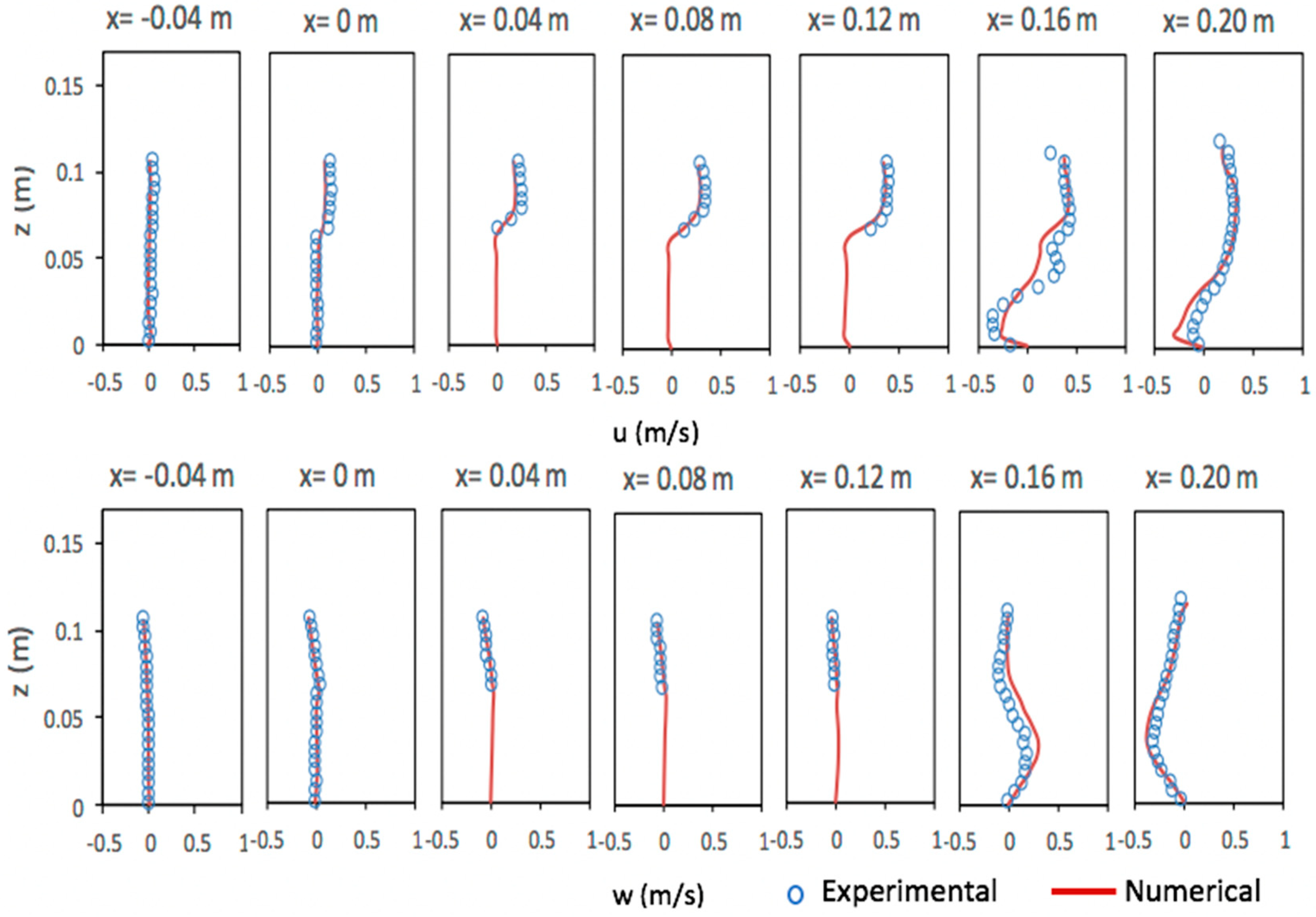
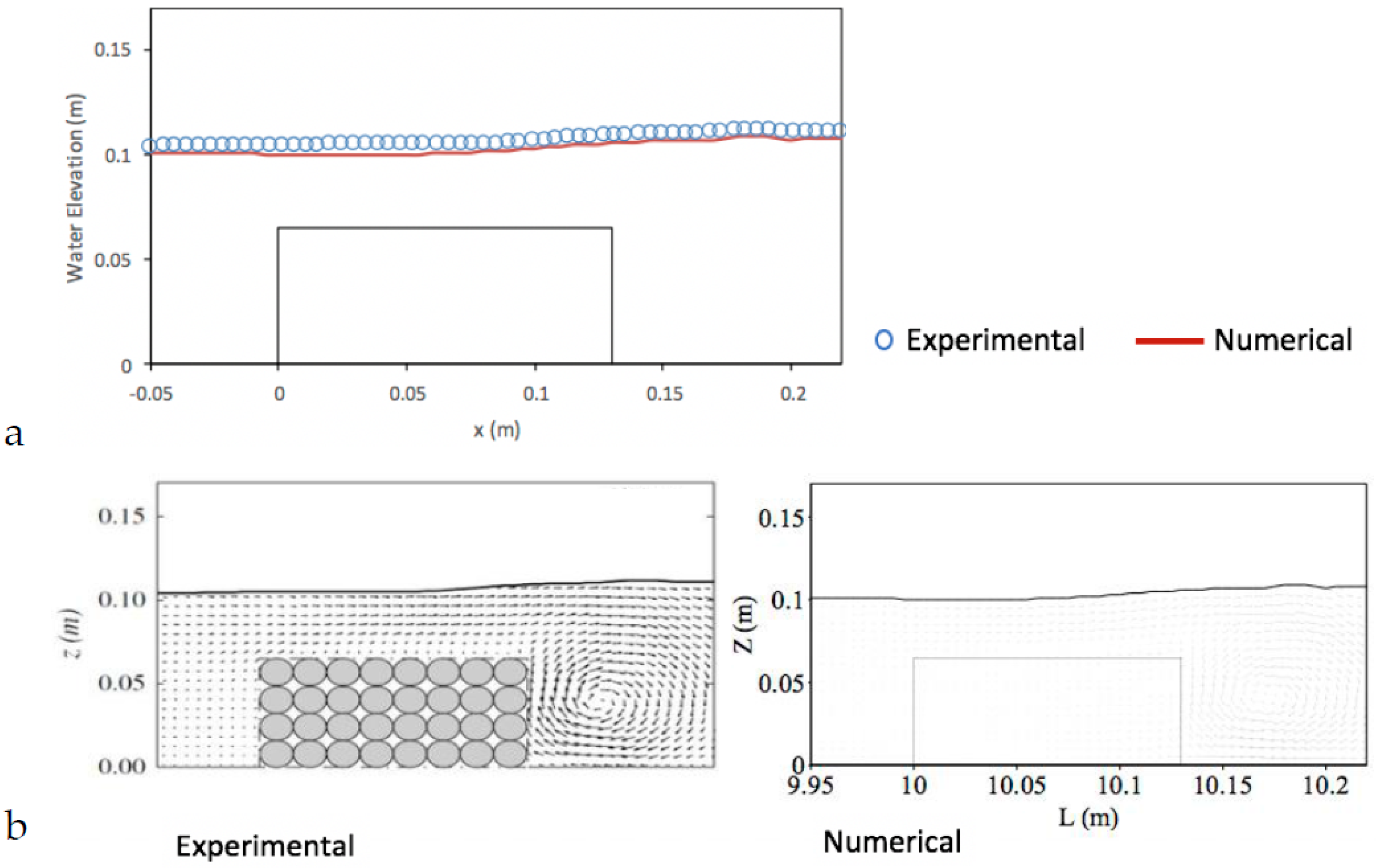
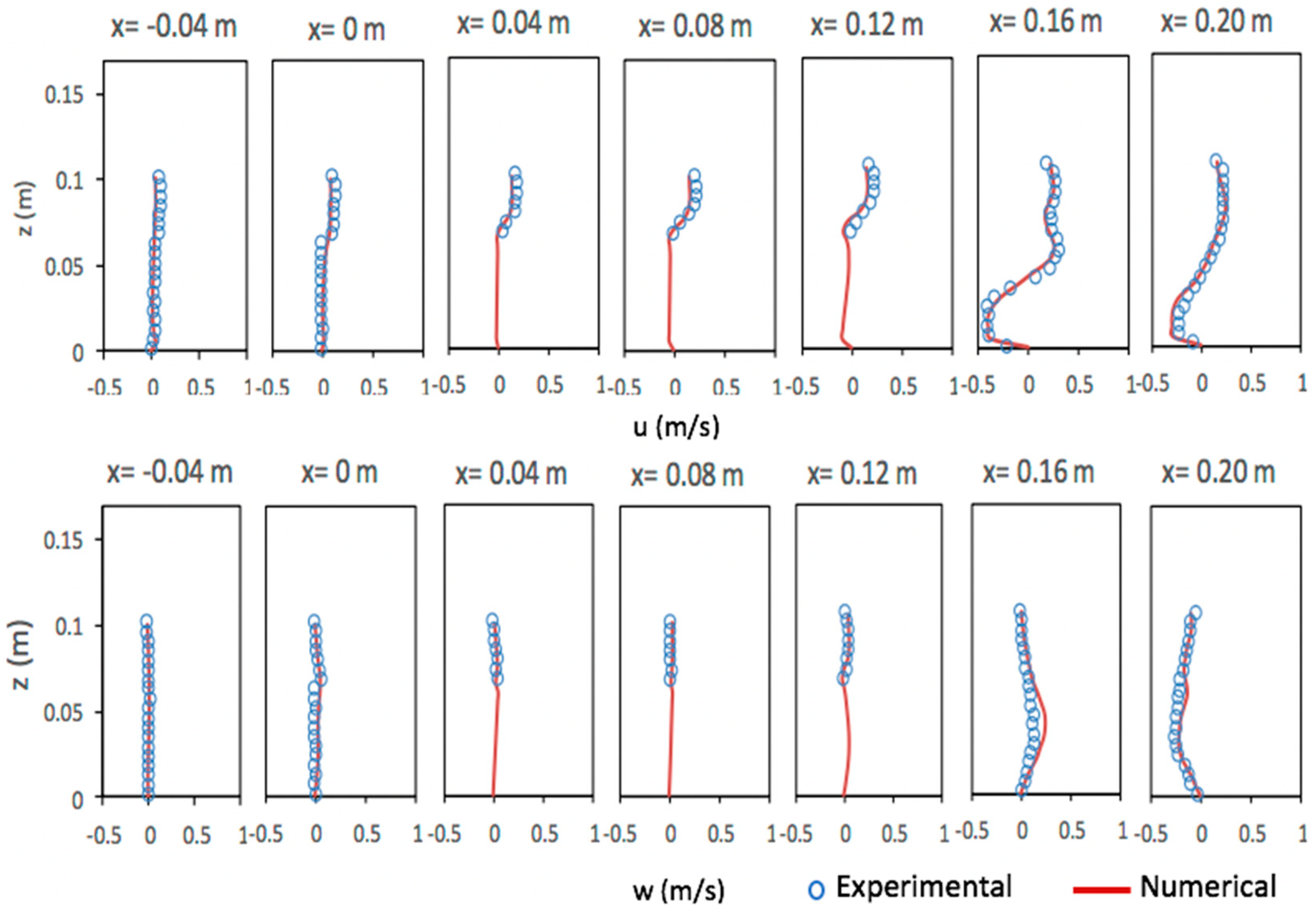
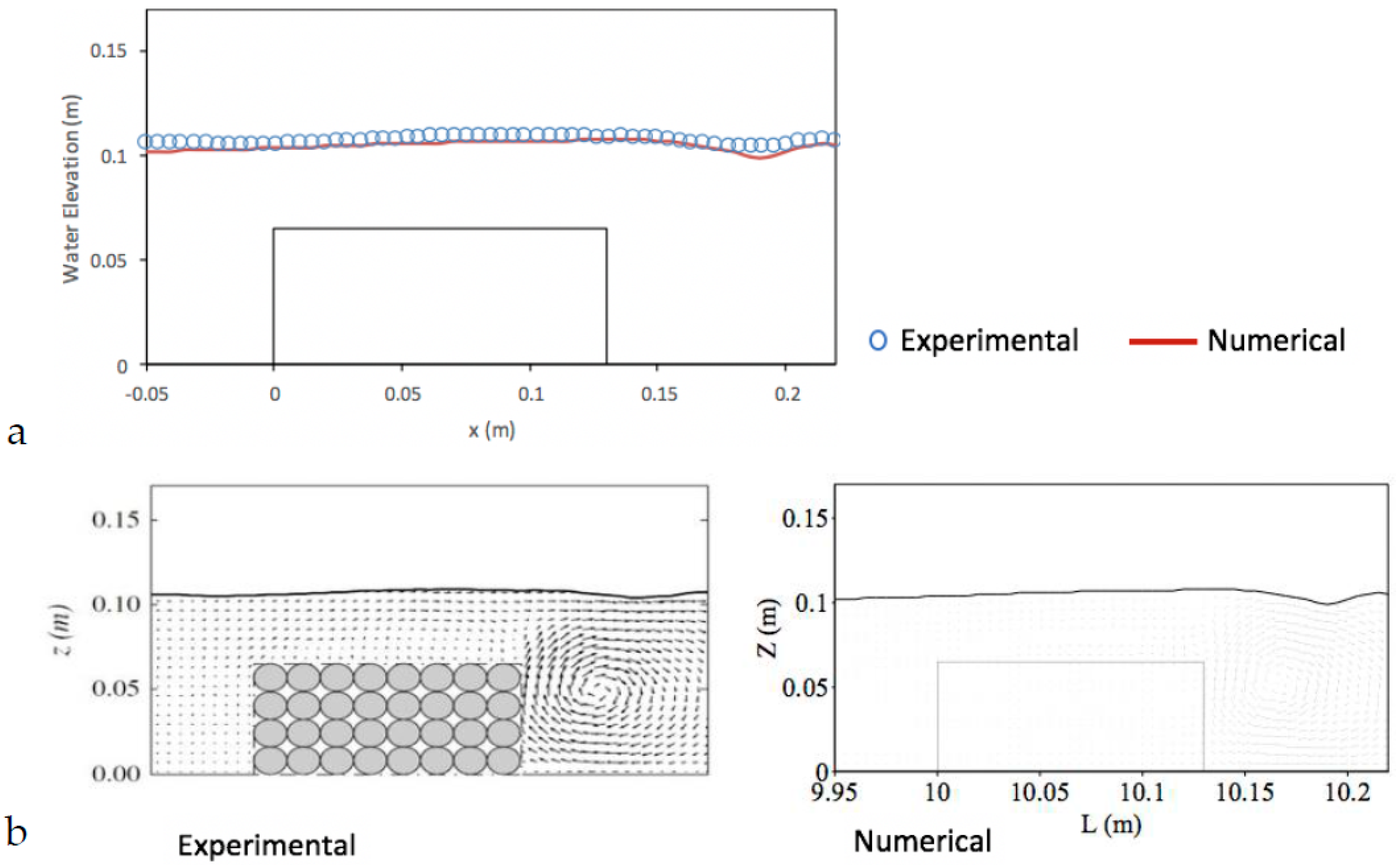
5.3. Solitary Wave Interaction with a Permeable Submerged Breakwater

In this section, the newly developed model was deployed to investigate the solitary wave propagation over a submerged permeable breakwater. Numerical outputs were compared with the experimental data presented by Wu and Hsiao (2013). The experiment was conducted in a wave tank with the length of $L=25 \mathrm{m}$ and a permeable submerged structure with the length of $a=13 \mathrm{cm}$ and height of $b=6.5 \mathrm{cm}$ was situated at the bottom. The breakwater was made of glass spheres with a diameter of $D=1.5 \mathrm{cm}$, yielding a total porosity of $n=0.52$. A solitary wave with a height of $H=4.77 \mathrm{cm}$ propagated in a water depth of $h=10.6 \mathrm{cm}$. The PIV method was utilized for the experimental measurements of flow field around the porous structure. The origin of the coordinate system was assumed to be at the intersection of the impermeable bed and the left side of the breakwater. The time series of the surface displacement was measured by two capacity gauges located at $x=-1.8 \mathrm{m}$ and $x=1.8 \mathrm{m}$. In calculations, the time $t=0 \mathrm{s}$ was defined as the time when the solitary wave crest reached the first gauge. Figure 7 shows the schematic description of the numerical wave tank.

The length of wave tank was discretized with uniform grids of $\Delta x=0.005 \mathrm{m}$, and $20$ layers were considered over the depth of calculation domain. The total simulation time was $t=25 \mathrm{s}$ and the time interval was chosen to be $\Delta t=0.001 \mathrm{s}$. The coefficients $C_D$ and $C_M$ that produced the best agreement with the experimental measurements were considered as the calibration parameters in the numerical simulation. A number of values for each coefficient were considered and the effect of each individual parameter was studied by varying one coefficient while keeping another one unchanged and calculating the root mean square error (RMSE) for each set. In this study, the set of $C_D=3.5$ and $C_M=0.5$ resulting in the minimum RMSE was utilized for the numerical calculations. Figure 8 illustrates the comparison between experimental and numerical time histories of surface displacement at the location of measurement gauges.

As shown in Figure 8, the computed outputs agreed fairly well with the measured outputs for the incident, reflected, and transmitted waves.

Figure 9, Figure 10, Figure 11, Figure 12, Figure 13, Figure 14, Figure 15, Figure 16, Figure 17 and Figure 18 show the comparison between numerical predictions and experimental measurements for the spatial free surface distributions, velocity fields, and velocity profiles at five different time levels. According to the modelled and measured results, when the solitary wave front reached the permeable submerged breakwater, due to the hydraulic jump formation, the flow was separated from the top of the obstacle and small clockwise vortices were generated at the leading edge of the obstacle (Figure 9). When the solitary wave passed over the structure, a primary vortex was generated on the lee side of the structure (Figure 11). This vortex grew in size and penetrated into the deeper layers of water by increasing time (Figure 13). On the basis of the last two phases, the primary vortex gradually reached the free surface, lost its strength, and finally faded away due to the diffusive effects (Figure 15 and Figure 17). It is also seen that due to the resistance forces of the porous medium, the velocity inside the structure was substantially smaller than the velocity values on the top of the obstacle.

Comparisons between numerical model predictions and experimental measurements by Wu and Hsiao [23] show the capability of the newly developed model for the simulation of wave interactions with permeable submerged structures.

6. Conclusions

Extended Navier–Stokes equations with a non-hydrostatic pressure distribution were solved numerically in the whole computational domain to investigate the wave interactions with permeable submerged structures. The impact of porous medium was considered by including additional terms for drag and inertia forces into general Navier–Stokes equations. Finite volume method (FVM) in an arbitrary Lagrangian–Eulerian (ALE) formulation was utilized for the discretization of the numerical domain, in which the number of layers was constant during the whole calculations and the new mesh was generated after updating the surface elevation at each time step. The porosity components were updated by calculating the fraction of cell open to water and the total porosity of porous medium. Projection method was used to solve the extended Navier–Stokes equations in two main steps. In the first step, the Navier–Stokes equations in the absence of pressure gradients were solved to calculate an intermediate velocity field, which did not satisfy the continuity equation. In the second step, the continuity and momentum equations in the absence of advection, diffusion, and drag force terms were solved, and the pressure Poison equations were obtained for the computational grids below the top layer. The pressure equation for the computational cells located at the free surface layer was obtained by integrating the continuity equation over the depth and considering appropriate boundary conditions for the impermeable bed and free surface. The newly developed model in the absence of porous medium was firstly validated against analytical solutions of second-order Stokes and solitary wave propagation under non-breaking conditions. Numerical results agreed well with the analytical solutions. The model was then deployed for the simulation of a solitary wave passing over a rectangular porous structure. Numerical predictions for the time histories and spatial distribution of the free surface elevations, velocity fields, and velocity profiles were compared with the reported experimental measurements using the PIV method. Results showed that when the solitary wave reached the permeable submerged breakwater, a hydraulic jump was formed and the flow was separated from the top-left corner of the breakwater. When the solitary wave passed over the obstacle, a primary vortex was created behind the breakwater, which grew in time and penetrated into the bottom of the wave tank. This vortex gradually reached the upper layers of water and decreased in strength and finally disappeared due to the diffusive impacts. Comparisons between numerical results and experimental data proved the capability of the newly developed model in simulating the integrated fluid-porous medium problems and the interaction of wave with submerged breakwaters.

References

1. Sollitt, C.K.; Cross, R.H. Wave transmission through permeable breakwaters. In Proceedings of the 13th International Conference on Coastal Engineering, Vancouver, BC, Canada, 10–14 July 1972; pp. 1827–1846. [Google Scholar]
2. Rojanakamthorn, S.; Isobe, M.; Watanabe, A. A Mathematical Model of Wave Transformation over a Submerged Breakwater. Coast. Eng. Jpn. 1989, 32, 209–234. [Google Scholar] [CrossRef]
3. Losada, I.; Silva, R.; Losada, M. Ángel 3-D non-breaking regular wave interaction with submerged breakwaters. Coast. Eng. 1996, 28, 229–248. [Google Scholar] [CrossRef]
4. Méndez, F.J.; Losada, I.J.; Losada, M.A. Wave-Induced Mean Magnitudes in Permeable Submerged Breakwaters. J. Waterw. Port Coastal Ocean Eng. 2001, 127, 7–15. [Google Scholar] [CrossRef] [Green Version]
5. Hsu, T.-W.; Chang, J.-Y.; Lan, Y.-J.; Lai, J.-W.; Ou, S.-H. A parabolic equation for wave propagation over porous structures. Coast. Eng. 2008, 55, 1148–1158. [Google Scholar] [CrossRef] [Green Version]
6. Kobayashi, N.; Otta, A.K.; Roy, I. Wave Reflection and Run-Up on Rough Slopes. J. Waterw. Port Coastal Ocean Eng. 1987, 113, 282–298. [Google Scholar] [CrossRef]
7. Kobayashi, N.; Wurjanto, A. Numerical model for waves on rough permeable slopes. J. Coast. Res. 1990, 7, 149–166. [Google Scholar]
8. Wurjanto, A.; Kobayashi, N. Irregular Wave Reflection and Runup on Permeable Slopes. J. Waterw. Port Coastal Ocean Eng. 1993, 119, 537–557. [Google Scholar] [CrossRef]
9. Van Gent, M. The modelling of wave action on and in coastal structures. Coast. Eng. 1994, 22, 311–339. [Google Scholar] [CrossRef] [Green Version]
10. Cruz, E.C.; Isobe, M.; Watanabe, A. Boussinesq equations for wave transformation on porous beds. Coast. Eng. 1997, 30, 125–156. [Google Scholar] [CrossRef]
11. Madsen, P.A.; Murray, R.; Sørensen, O.R. A new form of the Boussinesq equations with improved linear dispersion characteristics. Coast. Eng. 1991, 15, 371–388. [Google Scholar] [CrossRef]
12. Hsiao, S.-C.; Liu, P.L.-F.; Chen, Y. Nonlinear water waves propagating over a permeable bed. Proc. R. Soc. A Math. Phys. Eng. Sci. 2002, 458, 1291–1322. [Google Scholar] [CrossRef]
13. Chen, Q. Fully Nonlinear Boussinesq-Type Equations for Waves and Currents over Porous Beds. J. Eng. Mech. 2006, 132, 220–230. [Google Scholar] [CrossRef]
14. Hsiao, S.C.; Hu, K.C.; Hwung, H.H. Extended Boussinesq equations for water-wave propagation in porous media. J. Eng. Mech. 2009, 136, 625–640. [Google Scholar] [CrossRef]
15. Sakakiyama, T.; Kajima, R. Numerical simulation of nonlinear wave interacting with permeable breakwaters. Coast. Eng. Proc. 1992, 1. [Google Scholar] [CrossRef]
16. Van Gent, M.R.A. Wave Interaction with Permeable Coastal Structures. Ph.D. Thesis, Delft University of Technology, Stevinweg, The Netherlands, 1996; p. 27. [Google Scholar]
17. Liu, P.L.-F.; Lin, P.; Chang, K.-A.; Sakakiyama, T. Numerical Modeling of Wave Interaction with Porous Structures. J. Waterw. Port Coastal Ocean Eng. 1999, 125, 322–330. [Google Scholar] [CrossRef]
18. Hsu, T.-J.; Sakakiyama, T.; Liu, P.L.-F. A numerical model for wave motions and turbulence flows in front of a composite breakwater. Coast. Eng. 2002, 46, 25–50. [Google Scholar] [CrossRef]
19. Huang, C.-J.; Chang, H.-H.; Hwung, H.-H. Structural permeability effects on the interaction of a solitary wave and a submerged breakwater. Coast. Eng. 2003, 49, 1–24. [Google Scholar] [CrossRef]
20. Karunarathna, S.; Lin, P. Numerical simulation of wave damping over porous seabeds. Coast. Eng. 2006, 53, 845–855. [Google Scholar] [CrossRef]
21. Del Jesus, M.; Lara, J.L.; Losada, I.J. Three-dimensional interaction of waves and porous coastal structures: Part I: Numerical model formulation. Coast. Eng. 2012, 64, 57–72. [Google Scholar] [CrossRef]
22. Wu, Y.-T.; Hsiao, S.-C. Propagation of solitary waves over a submerged permeable breakwater. Coast. Eng. 2013, 81, 1–18. [Google Scholar] [CrossRef]
23. Ma, G.; Shi, F.; Hsiao, S.-C.; Wu, Y.-T. Non-hydrostatic modeling of wave interactions with porous structures. Coast. Eng. 2014, 91, 84–98. [Google Scholar] [CrossRef]
24. Bonovas, M.; Belibassakis, K.; Rusu, E. Multi-DOF WEC Performance in Variable Bathymetry Regions Using a Hybrid 3D BEM and Optimization. Energies 2019, 12, 2108. [Google Scholar] [CrossRef] [Green Version]
25. Belibassakis, K.; Bonovas, M.; Rusu, E. A Novel Method for Estimating Wave Energy Converter Performance in Variable Bathymetry Regions and Applications. Energies 2018, 11, 2092. [Google Scholar] [CrossRef] [Green Version]
26. Hejazi, K.; Soltanpour, M.; Sami, S. Numerical modeling of wave–mud interaction using projection method. Ocean Dyn. 2013, 63, 1093–1111. [Google Scholar] [CrossRef] [Green Version]
27. Chorin, A.J. Numerical solution of the Navier-Stokes equations. Math. Comput. 1968, 22, 745–762. [Google Scholar] [CrossRef]
28. Temam, R. Sur l’approximation de la solution des équations de Navier-Stokes par la méthode des pas fractionnaires (II). Arch. Ration. Mech. Anal. 1969, 33, 377–385. [Google Scholar] [CrossRef]
29. Yuan, H.; Wu, C.H. A two-dimensional vertical non-hydrostatic σ model with an implicit method for free-surface flows. Int. J. Numer. Methods Fluids 2004, 44, 811–835. [Google Scholar] [CrossRef]
30. Yuan, H.; Wu, C.H. An implicit three-dimensional fully non-hydrostatic model for free-surface flows. Int. J. Numer. Methods Fluids 2004, 46, 709–733. [Google Scholar] [CrossRef]
31. Dean, R.G.; Dalrymple, R.A. Water Wave Mechanics for Engineers and Scientists; World Scientific Publishing Company: Singapore, 1991; Volume 2. [Google Scholar]
32. Le Méhauté, B. An Introduction to Hydrodynamics and Water Waves; Springer Science & Business Media: Berlin/Heidelberg, Germany, 2013. [Google Scholar]
33. Lee, J.J.; Skjelbreia, J.E.; Raichlen, F. Measurement of velocities in solitary waves. J. Waterw. Port Coastal Ocean Div. 1982, 108, 200–218. [Google Scholar]
34. Lin, P. Numerical Modeling of Water Waves; Informa UK Limited: Colchester, UK, 2014. [Google Scholar]
Figure 1. Discretization of the computational domain using arbitrary Lagrangian–Eulerian (ALE) formulation.
Jmse 08 00087 g001
Figure 2. A partially filled control volume and the corresponding parameters.
Jmse 08 00087 g002
Figure 3. Comparison of surface displacement for a progressive Stokes wave at t = 140   s .
Jmse 08 00087 g003
Figure 4. Numerical and analytical surface predictions for a solitary wave propagating in a wave tank at different times of ( a )   t = 45   s , ( b )   t = 90   s , ( c )   t = 135   s , and ( d )   t = 180   s .
Jmse 08 00087 g004
Figure 5. Comparison between numerical results and analytical solutions for horizontal velocity component at different times of ( a )   t = 45   s , ( b )   t = 90   s , ( c )   t = 135   s , and ( d )   t = 180   s .
Jmse 08 00087 g005
Figure 6. Comparison between numerical results and analytical solutions for vertical velocity component at different times of ( a )   t = 45   s , ( b )   t = 90   s , ( c )   t = 135   s , and ( d )   t = 180   s .
Jmse 08 00087 g006
Figure 7. Representation of the wave tank.
Jmse 08 00087 g007
Figure 8. Comparison between measured and predicted time histories of free surface at ( a )   x = 1.8   m and ( b )   x = 1.8   m .
Jmse 08 00087 g008
Figure 9. Calculated results and experimental measurements of the (a) spatial surface elevation and (b) velocity fields at t = 1.45   s .
Jmse 08 00087 g009
Figure 10. Calculated results and experimental measurements of the velocity profiles at t = 1.45   s .
Jmse 08 00087 g010
Figure 11. Calculated results and experimental measurements of the (a) spatial surface elevation and (b) velocity fields at t = 1.65   s .
Jmse 08 00087 g011
Figure 12. Calculated results and experimental measurements of the velocity profiles at t = 1.65   s .
Jmse 08 00087 g012
Figure 13. Calculated results and experimental measurements of the (a) spatial surface elevation and (b) velocity fields at t = 1.85   s .
Jmse 08 00087 g013
Figure 14. Calculated results and experimental measurements of the velocity profiles at t = 1.85   s .
Jmse 08 00087 g014
Figure 15. Calculated results and experimental measurements of the (a) spatial surface elevation and (b) velocity fields at t = 2.05   s .
Jmse 08 00087 g015
Figure 16. Calculated results and experimental measurements of the velocity profiles at t = 2.05   s .
Jmse 08 00087 g016
Figure 17. Calculated results and experimental measurements of the (a) spatial surface elevation and (b) velocity fields at t = 2.25   s .
Jmse 08 00087 g017
Figure 18. Calculated results and experimental measurements of the velocity profiles at t = 2.25   s .
Jmse 08 00087 g018