Abstract
This paper is devoted to the random vibration analysis of jacket platforms under wave loads using the explicit time-domain approach. The Morison equation is first used to obtain the nonlinear random wave loads, which are discretized into random loading vectors at a series of time instants. The Newmark-β integration scheme is then employed to construct the explicit expressions for dynamic responses of jacket platforms in terms of the random vectors at different time instants. On this basis, Monte Carlo simulation can further be conducted at high efficiency, which not only provides the statistical moments of the random responses, but also gives the mean peak values of responses. Compared with the traditional power spectrum method, nonlinear wave loads can be readily taken into consideration in the present approach rather than using the equivalent linearized Morison equation. Compared with the traditional Monte Carlo simulation, the response statistics can be obtained through the direct use of the explicit expressions of dynamic responses rather than repeatedly solving the equation of motion. An engineering example is analyzed to illustrate the accuracy and efficiency of the present approach.
1. Introduction
Jacket platforms are the most widely used fixed offshore platforms in oil and gas exploitation, working at optimal operational water depths ranging from 100 to 200 m. The wave loads often dominate the environmental effects on jacket platforms. In particular, due to the increase in operational water depth, the natural frequencies of jacket platforms decrease and come close to the predominant frequencies of the wave energy, and the responses of jacket platforms are almost totally dependent on wave loads. To effectively support the topside facilities, the jacket structure is always fabricated as a welded tubular space frame consisting of vertical or battered legs strengthened by lateral bracing systems. Because the components of the jacket are slender cylinders with small diameters compared to the wavelength, the Morison equation can be applied to evaluate wave loads on jacket structures [1,2,3,4,5,6].
Wave loads are random in nature, and the responses of jacket platforms subjected to wave loads are random processes. Therefore, it is necessary to conduct random vibration analysis of jacket platforms to obtain the response statistics. Currently, the power spectrum method (PSM) is the dominant approach for random vibration analysis of jacket structures under random wave loads [7,8], in which the power spectra of random wave loads need to be determined first. However, the wave loads represented by the Morison equation are nonlinear functions of wave-particle velocities. To determine the power spectra of wave loads in terms of the power spectra of wave-particle velocity, it is required to conduct the statistical linearization of the nonlinear Morison equation, in which the mean square of the error between the nonlinear and the linearized form of the Morison equation is minimized [9,10]. It has been observed that the above statistical linearization technique will significantly underestimate the mean peak values of the dominating wave drags for high sea conditions [11]. In view of this, an alternative linearization principle can be adopted, in which the mean peak wave load in the nonlinear case is equated with that in the linear case [12]. Nevertheless, certain assumptions regarding the probability distribution of the amplitude of wave-particle velocity are required in the linearized process when using the new principle, which inevitably influences the accuracy of the mean peak values of structural responses.
To fully consider the nonlinear wave loads represented by the nonlinear Morison equation, the random vibration of jacket platforms should be conducted in the time domain. In this paper, the random response of a jacket platform subjected to wave loads is analyzed with the explicit time-domain method (ETDM), which was originally proposed for random vibration analysis of building and bridge structures subjected to random seismic excitations [13,14,15,16]. Instead of using the equivalent linearized Morison equation, the nonlinear random wave loads can be directly taken into consideration in ETDM without any difficulties. The Newmark-β integration scheme is first employed to establish the explicit expressions of dynamic responses of jacket platforms in terms of nonlinear random wave loads at different time instants. Using the explicit formulations of structural responses, Monte Carlo simulation (MCS) can then be conducted at high efficiency for achieving the statistical moments and the mean peak values of random responses [17], in which no repetitive solutions to the equation of motion are required for a large number of time-history analyses of the structure under different samples of wave loads. An engineering example involving a jacket platform with 11,688 degrees of freedom (DOFs) is analyzed to illustrate the accuracy and efficiency of the present approach.
2. Determination of Wave Loads with Nonlinear Morison Equation
Assume that the inclined cylinder C1C2, as shown in Figure 1, Figure 2 and Figure 3, is a typical component of a jacket platform submerged in sea water. In these figures, the x-direction refers to the direction of wave propagation, and the z-direction refers to the vertical direction with the origin O located at the static water level. The inclined angles of cylinder C1C2 with respect to the x-, y-, and z-direction are denoted as , , and , respectively, as also presented in Figure 1, Figure 2 and Figure 3. For an arbitrary point P(x, y, z) on cylinder C1C2, the wave-particle velocities along the x- and z-direction are denoted as and , respectively, for a two-dimensional swell model, and the corresponding wave-particle accelerations are denoted as and , respectively, as shown in Figure 1. For the same point P(x, y, z) on cylinder C1C2, the structural vibration velocities along the x-, y-, and z-direction are denoted as , , and , respectively, and the corresponding structural vibration accelerations are denoted as , , and , respectively, as shown in Figure 2. The cylinder C1C2 is subjected to wave loads, and the distributed wave loads acting at point P(x, y, z) along the x-, y-, and z-direction are denoted as , , and , respectively, as shown in Figure 3.
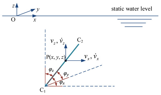
Figure 1.
Wave-particle velocities and accelerations at point P(x, y, z) on cylinder C1C2.
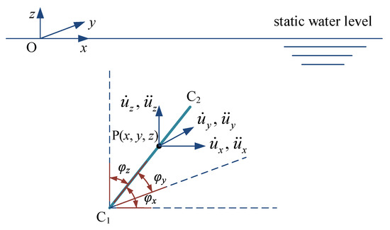
Figure 2.
Structural vibration velocities and accelerations at point P(x, y, z) on cylinder C1C2.
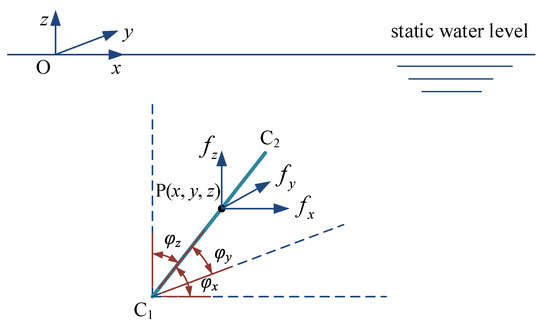
Figure 3.
Distributed wave loads acting at point P(x, y, z) on cylinder C1C2.
Using the nonlinear Morison equation and based on the quantities defined in Figure 1, Figure 2 and Figure 3, the total distributed wave loads can be derived as follows [18,19]:
where and ; ρ is the water density and D is the diameter of the cylinder; is the inertia coefficient and is the drag coefficient; is the added mass with being the added mass coefficient of the cylinder; m is the mass per unit length of the cylinder; is the distributed hydrodynamic damping matrix; and , , and are the three components of the wave-particle velocity normal to the cylinder, , which is defined as:
with .
Equation (1) can be rewritten in a more compact form as:
where is the total distributed wave loading vector, in which the superscript T denotes the matrix transposition; and , , , and represent the distributed added inertial force, hydrodynamic damping force, incident force and drag force vector, respectively, which are expressed as:
Note that in Equation (4) the drag forces in are nonlinear functions of the wave-particle velocities, and therefore the time-domain analysis, are required to consider the nonlinear drag forces.
3. Explicit Formulation of Dynamic Responses
3.1. Equation of Motion
The equation of motion for a jacket platform subjected to wave loads can be expressed as
where M, C, and K are the mass, damping, and stiffness matrix of the structure, respectively; , , and denote the nodal displacement, velocity, and acceleration vector of the structure, respectively; and L is the orientation matrix of the total concentrated wave loading vector , which can be determined through the distributed wave loads shown in Equation (3) and can be expressed as:
where , , , and are the concentrated added inertial force, hydrodynamic damping force, incident force, and drag force vector, respectively.
From the expressions of the distributed added inertial forces and hydrodynamic damping forces shown in Equation (4), and can be expressed in the following forms:
where and are the added mass matrix and the hydrodynamic damping matrix, respectively.
Substituting Equations (6) and (7) into Equation (5) yields:
where is the concentrated wave loading vector dependent on the wave-particle velocities and accelerations, which can be determined through the distributed incident forces and drag forces shown in Equation (4).
3.2. Explicit Time-Domain Expressions of Structural Responses
Define the state vector as . The recurrence formula for the state vector can be expressed as [13]:
where n is the number of time steps for time-history analysis; , , , and , in which , , and is the time step; and T, , and are the coefficient matrices derived through the Newmark-β integration scheme [14,15,16], which can be expressed as:
where I denotes the unit matrix; and β and γ are the two parameters associated with integration accuracy and stability, respectively. In this paper, β = 0.25 and γ = 0.50 are adopted for the unconditionally stable integration scheme.
Without loss of generality, assume and . Based on Equation (9), the explicit expression for the state vector of the jacket platform can be constructed in terms of the wave loading vectors at discretized time instants and can be written as follows [13]:
where are the coefficient matrices, which can be expressed in the closed forms as:
It can be seen from Equation (12) that, among the coefficient matrices, only needs to be calculated and stored, and the remainder can be obtained using the recurrence formula . Therefore, the calculation and storage of the coefficient matrices involved in the explicit formulation of structural responses can be readily achieved without significant effort.
From the perspective of engineering applications, only certain critical responses of offshore structures are of interest to engineers. Suppose that is one of the critical responses. With the explicit formulation of in Equation (11), the explicit time-domain expression of at time instant can be obtained as:
where:
in which represents the coefficient matrices shown in Equation (12); and is the response transfer row vector. When is the displacement or velocity of certain DOF, is a row vector consisting of 0 and 1; and when is an element force component, contains entries in the element force-displacement matrix.
4. Random Vibration Analysis with MCS Based on ETDM
4.1. Digital Simulation of Wave-Particle Velocities and Accelerations
To determine the drag and incident forces using Equation (4), the wave-particle velocities and accelerations are required, which are generally modeled as zero-mean stationary Gaussian random processes. Within the framework of linear random wave theory [20], the spectral representation method [17,21] is applied to the generation of wave-particle velocities and accelerations shown in Figure 1, which can be expressed as follows:
where is the power spectrum density function of the wave surface elevation; is the number of representative frequencies; is the i-th representative frequency and is the corresponding frequency interval; denotes the wave number of the i-th cosine wave; denotes the random phase angle of the i-th cosine wave with uniform distribution in [0, 2π]; and and are the depth-dependent functions given as:
in which h is the water depth of the sea site; and and should follow the dispersion relationship given as:
in which g is the gravitational acceleration.
The representative frequencies in Equations (15)–(18) should be arranged at non-uniform intervals so that small frequency intervals can be achieved around the peak value of , while larger intervals can be adopted at the frequency where the value of is small. In this regard, the representative frequencies can be obtained as follows [22]:
where denotes the average zero up-crossing period of the wave surface elevation.
4.2. ETDM-Based MCS
Once the samples of wave-particle velocities and accelerations are generated using Equations (15)–(18), the samples of the concentrated wave loading vector in Equation (8) can be obtained based on the distributed drag force vector and the distributed incident force vector shown in Equation (4). Thus far, the MCS for random vibration analysis of jacket platforms can be readily conducted based on the explicit time-domain expressions of structural responses presented in Section 3.2.
Suppose there is a total number of samples of the wave loading vector. For the k-th sample, , the prescribed critical response at different time instants can be obtained using Equation (13), which can be expressed as:
where , and are the coefficient row vectors shown in Equation (14).
Based on Equation (23), the mean and the variance of the critical response can be obtained as:
From a statistical perspective, the mean peak values of structural responses are generally used for the design purpose of a structure. The mean peak value of the critical response can be obtained as:
Note that the coefficient row vectors in Equation (23) need to be calculated just once and can be used for all of the sample analyses involved in MCS. This process has high efficiency compared with the traditional MCS, in which the equation of motion shown in Equation (8) needs to be solved for each sample of the wave loading vector. In addition, dimension-reduced MCS regarding certain critical responses of interest, rather than all the structural responses, can be easily conducted following Equation (23), which can further reduce the computational cost of MCS. To distinguish from the traditional MCS, the present approach can be termed ETDM-based MCS. For the sake of clarity, the solution procedure for the ETDM-based MCS is summarized in the flowchart presented in Figure 4.
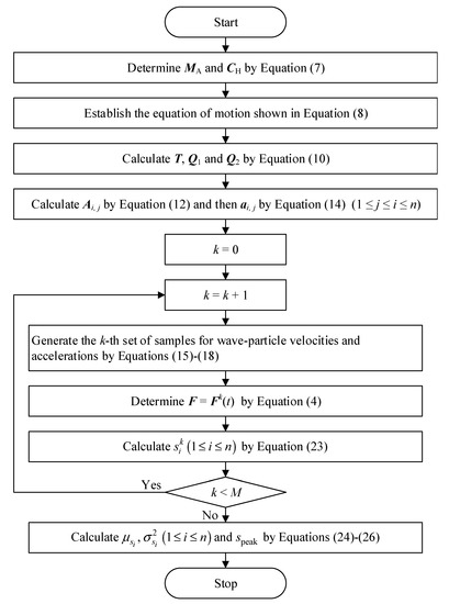
Figure 4.
Flowchart for the explicit time-domain method (ETDM)-based Monte Carlo simulation (MCS).
5. Numerical Example
5.1. Finite Element Model
In this section, the random responses of a steel jacket platform subjected to wave loads is investigated to illustrate the accuracy and efficiency of the present approach. The jacket platform is modeled with three dimensional beam elements, and the finite element (FE) model is shown in Figure 5. The height of the jacket platform is 86.80 m, and the depth of water is 62.00 m. The pile spacing is 25.00 m in the x-direction and 30.00 m in the y-direction. The fixed ends of the piles are set at a depth of six times the pile diameter from the bottom of the jacket platform. The whole model consists of 2303 beam elements and 1964 nodes, leading to a total number of 11,688 DOFs for the entire structure. The Rayleigh damping model is applied with the structural damping ratio being 2% for the steel jacket platform, and the hydrodynamic damping ratio can be taken as 8% according to a recent experimental investigation [18].
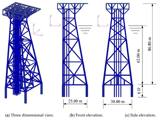
Figure 5.
The finite element (FE) model of the jacket platform.
5.2. Wave-Particle Velocities and Accelerations
The power spectrum density function of the wave surface elevation is taken to be the two-parameter Pierson–Moskowitz wave spectrum, which is particularly suited for open sea areas and is given mathematically as:
where is the significant wave height, and is the spectral peak frequency of the wave surface elevation. For a 100-year return period, and are set as 11.50 m and 0.44 rad/s, respectively, and the wave spectrum is shown in Figure 6.
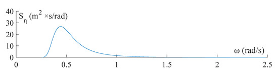
Figure 6.
Power spectrum density function of the wave surface elevation.
The velocities and accelerations of wave particles are generated with the spectral representation method based on Equations (15)–(18), in which 400 representative frequencies are considered in the range of 0.27 to 2.30 rad/s. A set of samples of wave-particle velocities and accelerations with a duration time of = 1000s are depicted in Figure 7 and Figure 8, respectively. To obtain the wave loads from the wave-particle velocities and accelerations, the hydrodynamic coefficients in Equation (4) are set as = 2.00 and = 1.30 [6,18].
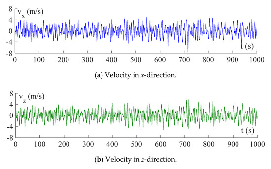
Figure 7.
Samples of wave-particle velocities on the sea surface.
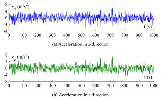
Figure 8.
Samples of wave-particle accelerations on the sea surface.
5.3. Deterministic Time-History Analysis with ETDM
Under the action of the wave-particle velocities and accelerations shown in Figure 7 and Figure 8, the deterministic time-history analysis of critical responses of the jacket platform is carried out with ETDM using Equation (13), in which the duration time of responses is set as = 1000 s with the time step set as ∆t = 0.20 s. For comparison, the time-history analysis is also conducted by solving Equation (8) directly with the Newmark-β method, in which = 1000 s and ∆t = 0.20 s. The time-histories of displacement and velocity at a top node of the jacket platform are shown in Figure 9a,b respectively, and the time-histories of bending stress and shear stress at the bottom of a battered leg are shown in Figure 10a,b, respectively. It can be seen from the above figures that the results obtained with ETDM are identical to those obtained with the Newmark-β method, indicating the correctness of the explicit formulation of structural responses in ETDM.
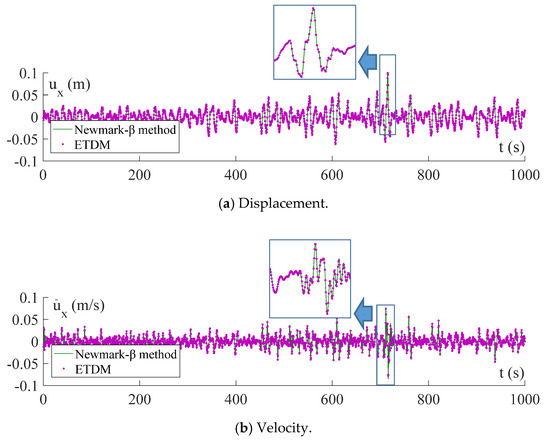
Figure 9.
Displacement and velocity at a top node of the jacket platform.
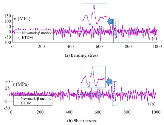
Figure 10.
Bending and shear stress at the bottom of a battered leg of the jacket platform.
5.4. Random Vibration Analysis with ETDM-Based MCS
The ETDM-based MCS stated in Section 4.2 is now used to conduct the random vibration analysis of the jacket platform with the nonlinear Morison equation, in which the samples of wave-particle velocities and accelerations are generated in Section 5.2 with a sample size of M = 1000. For the purpose of comparison, the PSM with the linearized Morison equation [9,10] is also used for the analysis of standard deviations of structural responses, and the mean peak value of a critical response is further obtained using the following equation [12]:
where is the standard deviation of the critical response; and denotes the number of wave cycles within the duration time under the consideration.
To investigate the influence of the linearization of the Morison equation on the response statistics of the jacket platform, different significant wave heights and spectral peak frequencies are considered in the above statistical analysis. The significant wave height is taken as 3.25, 5.00, 7.50, and 11.50 m, respectively, and the corresponding spectral peak frequency is taken as 0.76, 0.64, 0.53, and 0.44 rad/s, respectively. The standard deviations of displacement and velocity at a top node of the jacket platform are shown in Figure 11a,b, respectively, and the standard deviations of bending stress and shear stress at the bottom of a battered leg are shown in Figure 12a,b, respectively. The mean peak values of the above four critical responses are depicted in Figure 13 and Figure 14. It can be observed from Figure 11 and Figure 12 that the standard deviations of displacement and stress responses obtained with the two methods are in good agreement, while for the standard deviations of the velocity response, the discrepancy between the results of the two methods reaches up to 16%. Furthermore, in Figure 13 and Figure 14, with the increase in significant wave height, large discrepancies up to 94% can be found between the mean peak values of responses obtained with the two methods. The mean peak values are underestimated to a large extent by the method based on the linearized Morison equation for high sea conditions with dominating wave drags. This phenomenon is consistent with the observation reported in the literature [11,12].
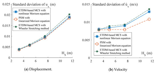
Figure 11.
Standard deviations of the displacement and velocity at a top node of the jacket platform.
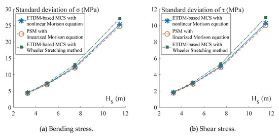
Figure 12.
Standard deviations of the bending and shear stress at the bottom of a battered leg of the jacket platform.
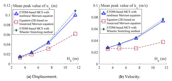
Figure 13.
Mean peak values of the displacement and velocity at a top node of the jacket platform.
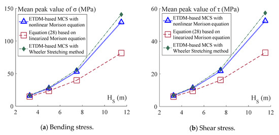
Figure 14.
Mean peak values of the bending and shear stress at the bottom of a battered leg of the jacket platform.
To further consider the influence on the jacket platform of the wave loads above the still water level, the Wheeler stretching method is used to modify the profiles of the wave-particle velocities and accelerations [23,24], and the wave loads are modified accordingly using Equation (4). The corresponding standard deviations and mean peak values of the four critical responses are obtained with ETDM-based MCS, which are also depicted in Figure 11, Figure 12, Figure 13 and Figure 14 for comparison. It can be observed from Figure 11, Figure 12, Figure 13 and Figure 14 that with the increase in the significant wave height, an increase up to 7% occurs in both standard deviations and mean peak values of the critical responses when the Wheeler stretching method is used to account for the effects of the wave loads above the still water level.
To investigate the computational efficiency, the time elapsed by ETDM-based MCS and the traditional MCS is presented in Table 1. It takes about 200 s to calculate the coefficient matrices for construction of the explicit expressions of dynamic responses, and then only a total time of 100 s is required for MCS with 1000 sample analyses based on the explicit formulation of responses. In contrast, the computation time for the traditional MCS reaches 106 s with the same sample size, in which the equation of motion of the structure needs to be solved for each sample analysis. It can be seen that the present ETDM-based MCS has high efficiency and can be effectively used for the time-domain random vibration analysis of jacket platforms under wave loads, in which the nonlinear Morison equation for the wave drags can be readily taken in consideration.

Table 1.
Computation time of ETDM-based MCS and the traditional MCS with 1000 sample analyses.
6. Conclusions
For jacket platforms under random wave loads, the time-domain MCS is considered the optimal choice for consideration of the nonlinear Morison equation of wave drags, and for evaluation of the mean peak values of stochastic responses without additional assumptions regarding the probability distribution of responses. However, the large computational cost obstructs the application of the traditional MCS to engineering practice. ETDM with explicit expressions of dynamic responses addresses the bottleneck of the extremely low efficiency of MCS and makes it feasible for practical application to engineering problems. In this paper, the ETDM-based MCS was applied to the random vibration analysis of a jacket platform with 11,688 DOFs subjected to random wave loads, indicating the high accuracy of the present approach compared with the method based on the linearized Morison equation, and the high efficiency compared with the traditional MCS.
Author Contributions
C.S. conceived the overall approach and the main conceptual design of the article. W.L. implemented the approach and drafted the manuscript. Y.T. helped with revising the content of the text. All authors have read and agreed to the published version of the manuscript.
Funding
This research was funded by the National Natural Science Foundation of China, grant number 51678252, and the Science and Technology Program of Guangzhou, China, grant number 201804020069.
Conflicts of Interest
The authors declare that they have no conflict of interest.
References
- Morison, J.R.; O’Brien, M.P.; Johnson, J.W.; Schaaf, S.A. The force exerted by surface waves on piles. J. Pet. Technol. 1950, 2, 149–154. [Google Scholar] [CrossRef]
- Det Norske Veritas. Environmental Conditions and Environmental Loads; DNV-RP-C205: Oslo, Norway, 2014. [Google Scholar]
- Boccotti, P.; Arena, F.; Fiamma, V.; Barbaro, G. Field experiment on random wave forces acting on vertical cylinders. Prob. Eng. Mech. 2012, 28, 39–51. [Google Scholar] [CrossRef]
- Boccotti, P.; Arena, F.; Fiamma, V.; Romolo, A. Two small-scale field experiments on the effectiveness of Morison’s equation. Ocean Eng. 2013, 57, 141–149. [Google Scholar] [CrossRef]
- Santo, H.; Taylor, P.H.; Williamson, C.H.K.; Choo, Y.S. The relative-velocity version of the Morison equation for obstacle arrays in combined steady, low and high frequency motion. J. Fluid Mech. 2018, 842, 188–214. [Google Scholar] [CrossRef]
- Santo, H.; Taylor, P.H.; Day, A.H.; Nixon, E.; Choo, Y.S. Current blockage and extreme forces on a jacket model in focused wave groups with current. J. Fluids Struct. 2018, 78, 24–35. [Google Scholar] [CrossRef]
- Taylor, R.E.; Rajagopalan, A. Load spectra for slender offshore structures in waves and currents. Earthq. Eng. Struct. Dyn. 2010, 11, 831–842. [Google Scholar] [CrossRef]
- Silva, L.S.P.D.; Cazzolato, B.S.; Sergiienko, N.Y.; Ding, B.; Morishita, H.M.; Pesce, C.P. Statistical linearization of the Morison’s equation applied to wave energy converters. J. Ocean Eng. Mar. Energy 2020, 6, 157–169. [Google Scholar] [CrossRef]
- Borgman, L.E. Random hydrodynamic forces on objects. Ann. Math. Stat. 1967, 38, 37–51. [Google Scholar] [CrossRef]
- Borgman, L.E. Spectral analysis of ocean wave forces on piling. J. Waterw. Harb. Div. 1967, 93, 129–156. [Google Scholar]
- Brouwers, J.J.H.; Verbeek, P.H.J. Expected fatigue damage and expected extreme response for Morison-type wave loading. Appl. Ocean Res. 1983, 5, 129–133. [Google Scholar] [CrossRef]
- Wolfram, J. On alternative approaches to linearization and Morison’s equation for wave forces. Proc. R. Soc. Lond. A Math. Phys. Eng. Sci. 1999, 455, 2957–2974. [Google Scholar] [CrossRef]
- Su, C.; Xu, R. Random vibration analysis of structures by a time-domain explicit formulation method. Struct. Eng. Mech. 2014, 52, 239–260. [Google Scholar] [CrossRef]
- Su, C.; Huang, H.; Ma, H.T. Fast equivalent linearization method for nonlinear structures under nonstationary random excitations. J. Eng. Mech. 2016, 142, 4016049. [Google Scholar] [CrossRef]
- Su, C.; Li, B.M.; Chen, T.C.; Dai, X. Stochastic optimal design of nonlinear viscous dampers for large-scale structures subjected to non-stationary seismic excitations based on dimension-reduced explicit method. Eng. Struct. 2018, 175, 217–230. [Google Scholar] [CrossRef]
- Su, C.; Liu, X.L.; Li, B.M.; Huang, Z. Inelastic response analysis of bridges subjected to non-stationary seismic excitations by efficient MCS based on explicit time-domain method. Nonlinear Dyn. 2018, 94, 2097–2114. [Google Scholar] [CrossRef]
- Shinozuka, M. Monte-Carlo solution of structural dynamics. Comput. Struct. 1972, 2, 855–874. [Google Scholar] [CrossRef]
- Santo, H.; Taylor, P.H.; Day, A.H.; Nixon, E.; Choo, Y.S. Blockage and relative velocity Morison forces on a dynamically-responding jacket in large waves and current. J. Fluids Struct. 2018, 81, 161–178. [Google Scholar] [CrossRef]
- Borgman, L.E. Computation of the ocean-wave forces on inclined cylinders. Trans. Am. Geophys. Union 1958, 39, 885–888. [Google Scholar] [CrossRef]
- Charkrabarti, S.K. Laboratory generated waves and wave theories. J. Waterw. Port. Coast. Ocean Eng. Div. 1980, 106, 349–368. [Google Scholar]
- Su, C.; Han, D.J.; Yan, Q.S.; Au, F.T.K.; Tham, L.G.; Lee, P.K.K.; Lam, K.M.; Wong, K.Y. Wind-induced vibration analysis of the Hong Kong Ting Kau Bridge. Proc. Inst. Civ. Eng.-Struct. Build. 2003, 156, 263–272. [Google Scholar] [CrossRef]
- Wang, D.J. Hydrodynamic Behavior of Large Moored Offshore Structures during Adverse Weather Conditions. Ph.D. Thesis, Hong Kong Polytechnic, Hong Kong, China, 1993. [Google Scholar]
- American Bureau of Shipping. Guidance Notes on Dynamic Analysis Procedure for Self-Elevating Drilling Units; American Bureau of Shipping: Houston, TX, USA, 2004. [Google Scholar]
- Wheeler, J.D. Method for calculating forces produced by irregular waves. J. Pet. Technol. 1970, 22, 359–367. [Google Scholar] [CrossRef]
Publisher’s Note: MDPI stays neutral with regard to jurisdictional claims in published maps and institutional affiliations. |
© 2020 by the authors. Licensee MDPI, Basel, Switzerland. This article is an open access article distributed under the terms and conditions of the Creative Commons Attribution (CC BY) license (http://creativecommons.org/licenses/by/4.0/).