Article

Pressure Signal Analysis for the Characterization of High-Viscosity Two-Phase Flows in Horizontal Pipes

by
Lizeth Torres
1,
José Noguera
2,
José Enrique Guzmán-Vázquez
1,*,
Jonathan Hernández
1,
Marco Sanjuan
2 and
Arturo Palacio-Pérez
1
1
Instituto de Ingeniería, Universidad Nacional Autónoma de México, Mexico City 04510, Mexico
2
Departamento de Mecánica, Facultad de Ingeniería, Universidad del Norte, Barranquilla 081007, Colombia
*
Author to whom correspondence should be addressed.
J. Mar. Sci. Eng. 2020, 8(12), 1000; https://doi.org/10.3390/jmse8121000
Submission received: 13 November 2020 / Accepted: 18 November 2020 / Published: 8 December 2020
(This article belongs to the Special Issue Offshore Oil and Gas Transportation)

Abstract

:
We study a high-viscosity two-phase flow through an analysis of the corresponding pressure signals. In particular, we investigate the flow of a glycerin–air mixture moving through a horizontal pipeline with a U-section installed midway along the pipe. Different combinations of liquid and air mass flow rates are experimentally tested. Then, we examine the moments of the statistical distributions obtained from the resulting pressure time series, in order to highlight the significant dynamical traits of the flow. Finally, we propose a novel correlation with two dimensionless parameters: the Euler number and a mass-flow-rate ratio to predict the pressure gradient in high-viscosity two-phase flow. Distinctive variations of the pressure gradients are observed in each section of the pipeline, which suggest that the local flow dynamics must not be disregarded in favor of global considerations.

1. Introduction

Highly viscous gas-liquid flows occur in regions where extra-heavy oils (< 10 API1), such as those obtained from bitumen oil sands [1,2], constitute a relevant share of the actual production [3]. According to recent estimates, nearly 50% of the technically recoverable heavy oil reserves have gravities below 15 API, while the fields producing them are observed to grow 5 times faster than the fields producing conventional (i.e., high API) crude oils [2,4]. However, because of their particular composition and viscosity, flows of this type present challenging problems during the operation of onshore and offshore pipelines [5,6,7]. Concretely, the recovery of heavy and extra heavy crude oils, as well as the transportation through pipelines, is hindered by their low mobility.
Apart from the flow assurance problems caused by the formation of solid deposits and scaling, high viscosity flows entail an increased damaging potential to the transportation system. Chronic pipe fatigue (i.e., the weakening of the pipe material caused by cyclic loading [8]), as well as corrosion and erosion processes enhanced by high intermittent pressures may lead to failures with severe economical and environmental consequences (e.g., [9,10,11]). A recent survey indicates that much of the work has focused on improving models, measuring techniques and control methods. Deep water applications are particularly challenging [6]. The salient point of this review is the lack of robustness of the flow control methods, which are ultimately related with the slugging processes.
Work carried out along these lines clearly shows that high-viscosity regimes are characterized by flow patterns that differ from those previously established for low viscosity mixtures. In fact, most of the available experimental evidence suggests that the predominant pattern is intermittent in nature [12,13,14]. Under these circumstances, the relevant flow parameters exhibit a strong dependence on the viscosity of the mixture [15,16,17,18]. Concretely, the recent work by Archibong-Eso et al. (2019) dealt with gas–liquid flows in the viscosity range from 0.189 to 5.0 Pa s (189 to 5000 cP), at the experimental temperature, in flow loops with an internal diameter of 0.076 m [19]. The flow system and the process are similar to the ones discussed in this paper, but the authors focus on analyzing the liquid holdup. A new correlation was proposed to account for a wide range of high viscosity fluids, including the effect of pipe diameter.
Another set of experiments carried out with oil–air mixtures, whose viscosities ranged from 1.0 to 5.5 Pa s (1000 cP to 5500 cP), showed that the slug length decreases with increasing viscosity [20]. Similarly, the bubble velocity and other slug properties have been the subject of dedicated analyses and modeling. In the high-viscosity interval from 0.1 to 1.0 Pa s (100 cP to 1000 cP), the bubble velocity can still be predicted by the Nicklin et al. correlation with corrections for the radial distribution coefficient and drift velocity, in terms of the Froude number [21]. A year earlier, Baba et al. (2017) analyzed the slugging frequency with flows in analogous experimental conditions [22]. The effects caused by slight inclinations of the flow pipe were studied by Ekinci et al. (2017) [23]. In this case, the viscosity under consideration was in the range from 0.155 to 0.587 Pa s (155 to 587 cP), while other characteristics of the experimental setup were the same as those discussed in the two preceding references. Their respective findings concern the flow patterns, liquid holdups, frequencies, and pressure gradients, for horizontal and slightly inclined pipes. We note that the general trends for the pressure gradients resemble the ones reported here, due to the similarity of the test section.
Al-Safran et al. (2015) also investigated the liquid holdup of gas-liquid flows in a dedicated experiment conducted in a 18.9 m long flow loop with an internal diameter of 0.05 m [24]. The viscosity of the liquid phase in that case was as high as 0.587 Pa s, and it was found that the holdup decreases (rapidly) with increasing viscosity. As a result of the analysis, a successfully validated model was proposed to evaluate the holdup in this viscosity limit. Finally, the study by Farsetti et al. (2014) concerns the flow of a 0.896 Pa s liquid-gas mixture moving through a (smaller) 0.02 m diameter pipe at different inclinations [25]. They estimated the pressure drop by means of the Chisholm correlation in terms of the Lockhart-Martinelli parameter. Based on the measurements, the pressure gradient appeared to be relatively insensitive to the superficial air velocity, while it was nearly directly proportional to the liquid superficial velocity. Matsubara and Naito (2011) analyzed the flow pattern transitions in a test facility with a similar layout (i.e., with a length of 19 m and an internal diameter of 0.02 m) [26]. They concluded that the stratified and the roll wave patterns are replaced by the annular and intermittent flows.
In the present work we are concerned with the characteristic fluctuations of the pressure fields produced by hydrodynamic slugging. The two-phase flow consists of a glycerin-air mixture with a viscosity of 0.9 Pa s (900 cP), which evolves in a horizontal pipe with a relatively large length-to-diameter ratio. The characterization is based on the statistical moments of the probability distributions of the pressure time-series, which were measured at three different sections along the pipe.
In addition, algorithms for two-level waveforms are used for analyzing the intermittency of the pressure signals. This analysis underlines the convenience of using root-mean-square (RMS2) values for characterizing intermittent flows, instead of their mean values. Accordingly, we propose a correlation for predicting the pressure gradients for similar flows in horizontal pipes.

2. Experimental Methods

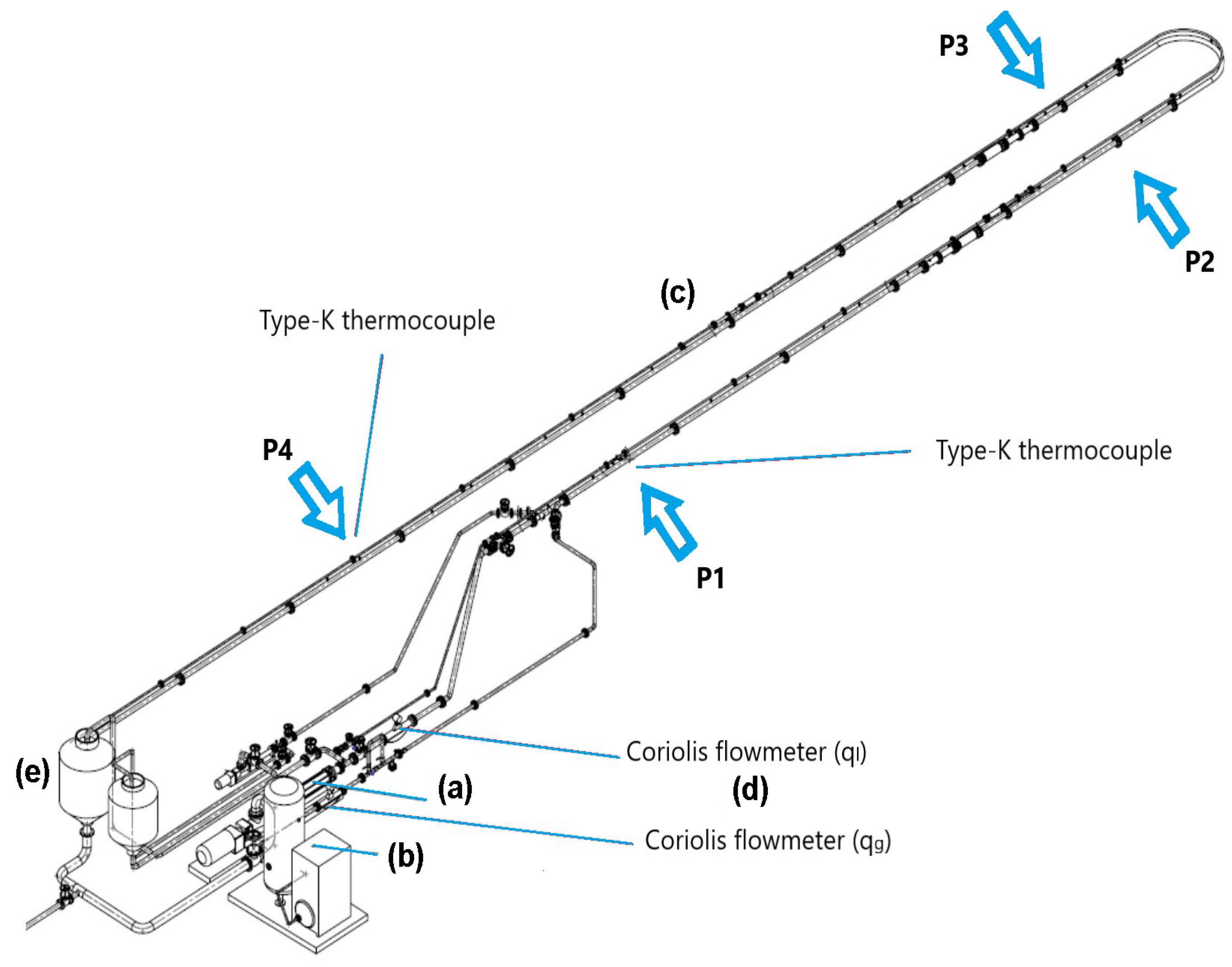
The experiments were conducted in a flow loop especially designed to analyze the (relatively long-term) development of highly viscous gas-liquid mixtures. Snapshots of the apparatus are shown in Figure 1, while the diagram of Figure 2 illustrates the arrangement of the flow control and measuring devices. The overall length of the horizontal test section was L = 54 m. Its modular design accommodated 3 m long (schedule 80) steel tubes, with an internal diameter D = 0.0762 m (3 in). A single transparent PVC tube (with the same internal radius) was fitted 6 m upstream from the discharge plane for visualization purposes. Note that a 4 m long U-section was located midway between the inlet and the outlet legs of the test section (Figure 2).
Newtonian fluids were used for convenience. The high-viscosity liquid of choice was glycerin with a dynamic viscosity μ = 0.99 Pa s (990 cP), density ρ = 1.24 × 10 3 kg/m 3 , and surface tension σ = 6.3 × 10 2 N/m. On the other hand, the gaseous phase was air with dynamic viscosity μ = 1.8 × 10 5 Pa s (0.018 cP) and density ρ = 1.02 kg/m 3 . These values correspond to the approximate conditions prevailing inside the laboratory during the tests, namely P 8.73 × 10 4 Pa and T 24 C.
The glycerin was injected into the flow loop by a Seepex BN35-24 progressive cavity pump, while a twin-scroll Käser Aircenter SK.2 Compressor supplied the air. An accumulation tank, a pressure regulator, and a globe valve allowed for a fine-tuned injection of a constant amount of air. Coriolis meters were used to measure both mass flow rates. An Endress–Hauser Promass 83F80 DN80 3” meter was used for the liquid, while a Promass 83F50 DN50 2” was used for the air. Their respective accuracies were 0.1% and 0.05% throughout the corresponding measuring intervals. The experiments were produced in accordance with the (inlet) mass flow rates indicated in Table 1. Nine flow rate combinations ( Q l , Q g ) were considered. The resulting mixture was discharged into a separator tank. Care was taken to avoid recycling glycerin with gas bubbles that were entrained as a result of the mixing process.
MEAS U5300 pressure transducers were installed at 0, 18, 22, and 43 m, downstream from the inlet (Figure 2). All pressures were measured with an accuracy of 0.1% within the 0.0 to 3.45 × 10 5 Pa interval. The temperature of the mixture was simultaneously measured near the inlet and outlet planes of the pipe, by means of type-K thermocouples with a resolution of 0.5 C. In addition, samples of the mixtures were extracted during each test to verify their actual viscosity values with a Brookfield DV2T viscometer.
The experiments were carried out according to the following procedure: (a) the glycerin was pumped at the selected Q l until a steady-state was reached, (b) the air was injected with the prescribed Q g , (c) the mixture was allowed to evolve until the average pressure registered at the inlet reached a stationary value, (d) the measurements were registered with the IMC Chronos-Flex CRFX-2000 acquisition system, and (e) the collected data was processed in a PC.
Table 2 shows the symbol definitions required for the computations of the pressure gradients reported in the results section. The actual values of the pressure drop in each leg depend on the instantaneous measurements.

3. Results

For clarity the snapshots of Figure 3 show the details of slug’s mixing front and trailing bubble.
The gas entrained at the mixing front leads to the formation of large bubbles within the slug, which are severely stretched as they are dragged along by the liquid (Figure 3a,b). At the opposite end of the slug body, the trailing bubble penetrates the slug, thereby creating a persistently-thick layer of liquid around it (Figure 3c). A combination of rounded and elongated bubbles coexist inside this layer, until the larger bubbles finally burst (Figure 3d). Note that a number of smaller bubbles remain attached to the fluid layer. These specific traits are markedly different from those observed with low viscosity mixtures and, therefore, modify the nature of the pressure field. We analyze the pressure in the following sections.

3.1. Statistical Characterization of the Pressures

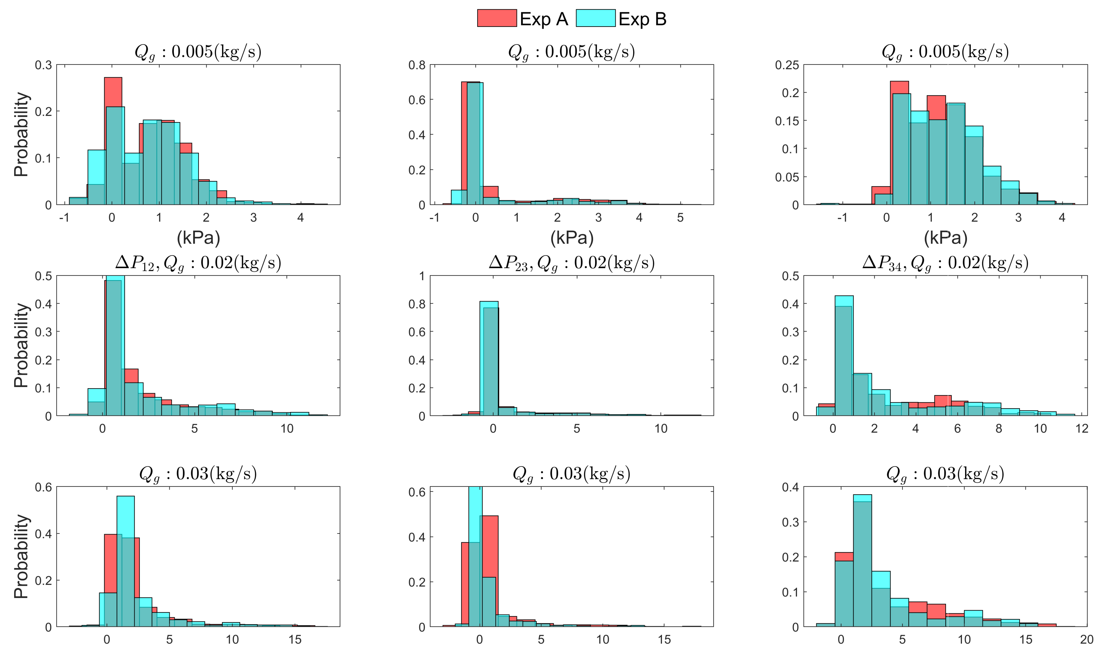
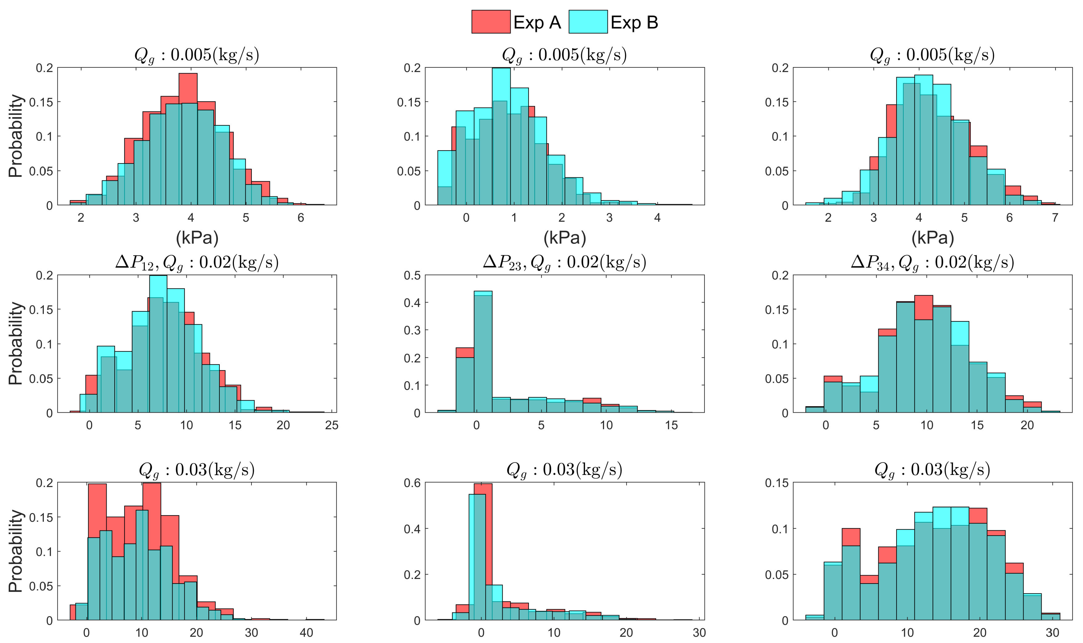
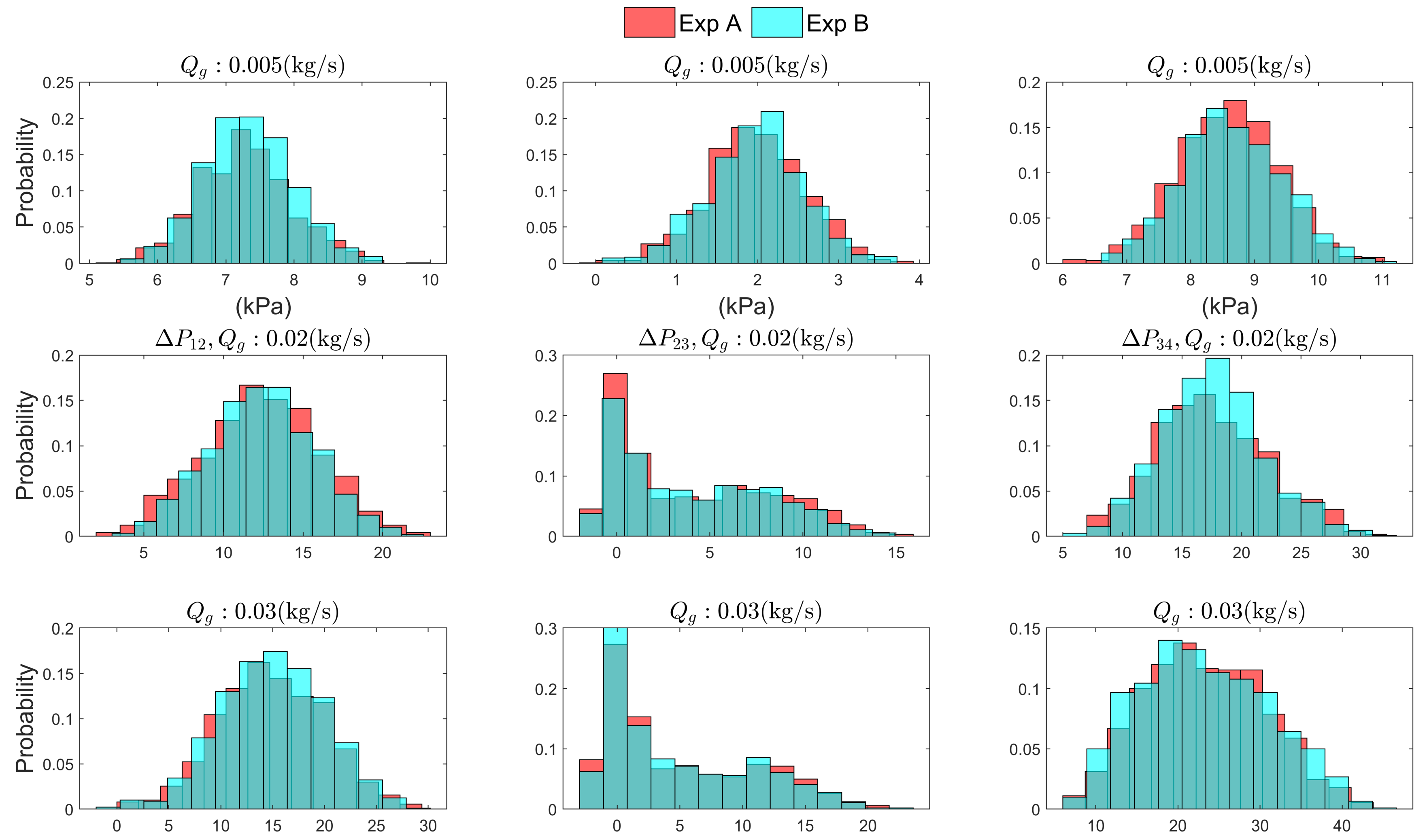
Figure 4, Figure 5 and Figure 6 show the general features of the pressure drop distributions. According to Akagawa et al. [27], the ( Δ P ) distribution depends on the length of the section where the pressure measurements are taken. Therefore, the data for Δ P 12 and Δ P 34 tend to have a similar behavior on the two long sections of the pipe, since Δ x 1 Δ x 3 . However, the shapes of the Δ P 23 distributions in the U-section of the pipe tend to be less distorted with higher flow rates (particularly for ( Q l = 3.7 , Q g = 0.03 ) kg/s and ( Q l = 6.1 , Q g = 0.03 ) kg/s, as Figure 5 and Figure 6 show). Apparently, the secondary flows induced by the centripetal acceleration of the mixture have a stabilizing effect.
The quantitative information obtained from these distributions is useful and provides an clearer overall picture. Table 3 shows the mean pressure drop in the three sections of the pipe. As expected, the mean values rise when either of the two mass flow rates increases, with Q l causing a far more significant effect than Q g . If the pressure drops are normalized in terms of their maximum values registered in a particular section of the pipe, that is if Δ P i j Δ P i j * = Δ P i j / max { Δ P i j } , then we observe: (a) an almost linear dependence of Δ P on Q l and Q g , and (b) this linear dependence is approximately valid in all pipe sections (see Table 4). Thus, in principle, this underlying pattern could be conveniently exploited to estimate the mean pressure at any point by means of non-local pressure measurements and inlet mass flow rates.
The standard deviation, on the other hand, increases linearly with Q g and behaves non-linearly with Q l (Table 5). This means that Δ P fluctuates more uniformly as Q g increases. In contrast, the fluctuation amplitudes increase substantially with Q l , but seem to asymptotically approach an upper limit. The overall effect is a kind of statistical regularization of the pressure field.
The relative importance of extreme Δ P values contained in the measurements is suitably quantified by the kurtosis of the corresponding distribution. Table 6 summarizes the kurtosis for the respective pressure drop distributions in each section of the pipe. The salient feature is that the lowest ( Q l , Q g ) combinations produce the largest amount of extreme pressure fluctuations. Conversely, high mass flow rates significantly reduce the extreme fluctuations.
The manner in which the low and high pressure fluctuations are arranged about the mean is best described by the skewness of the distributions. From the data reported in Table 7 it is clear that, in almost all cases, a greater number of fluctuations occur above the mean pressure. This asymmetry appears to be caused by the overdamped motion of the slug system, which in turn is promoted by the appearance rarefaction waves. In contrast, the collective motion of the slug units would be underdapmed in the low viscosity regime.

3.2. Characterization of Pressure Gradients

Various efforts have been made to obtain a unique correlation to predict the pressure gradient in two-phase flow similar to that of single-phase flow. Any proposed correlation should preferably be expressed using dimensionless parameters and present data on a single graph. In this spirit, and based on the work of Al-Sarkhi and Sarica [28], we propose a new correlation based on the Euler number, Eu, and the mass-flow-rate ratio Q l / Q g . First, we consider the pressure gradients along Δ x 1 , Δ x 2 and Δ x 3 for the different combinations of Q l and Q g to highlight their local behavior.
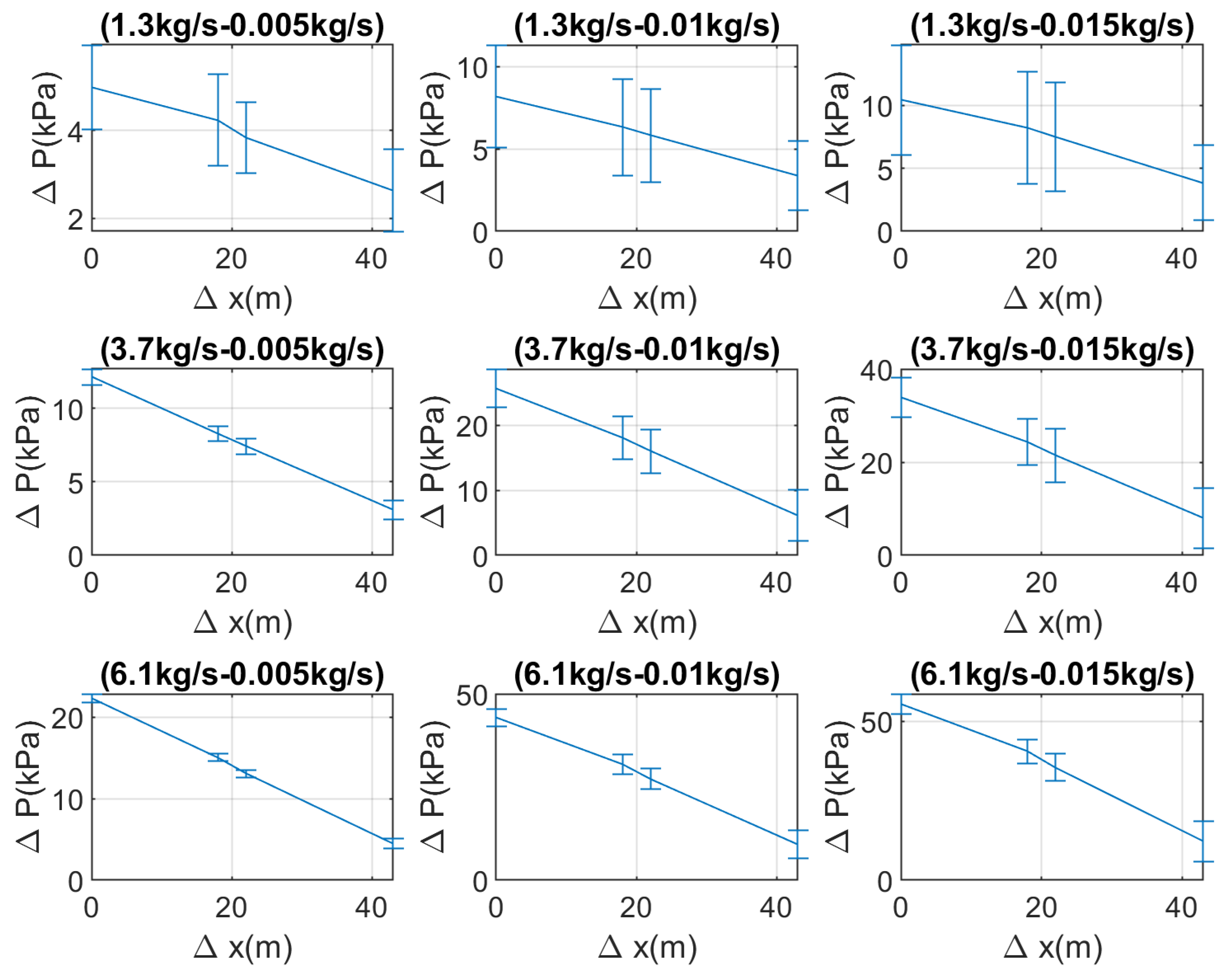
Generally speaking, the average pressure gradients are different in each of the three sections of the pipeline. Figure 7 illustrates this situation with plots for Δ P 12 , Δ P 23 and Δ P 34 for all combinations of glycerin and air mas flows rates. The specific Δ P i / Δ x i values summarized in Table 8 and Table 9 lead to the following observation: the greatest differences between pressure gradients are produced with the highest liquid and gas mass-flow rates.
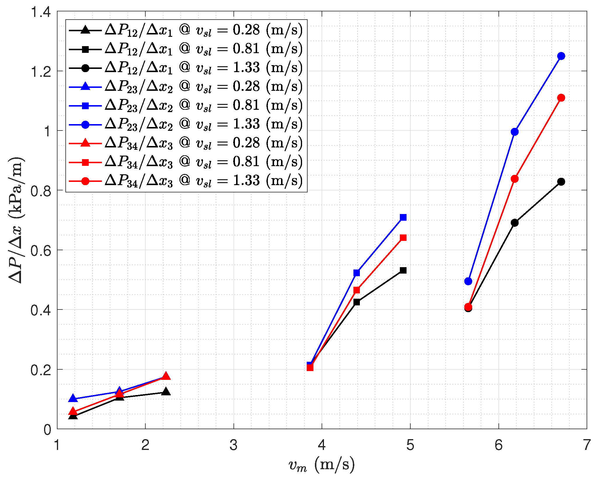
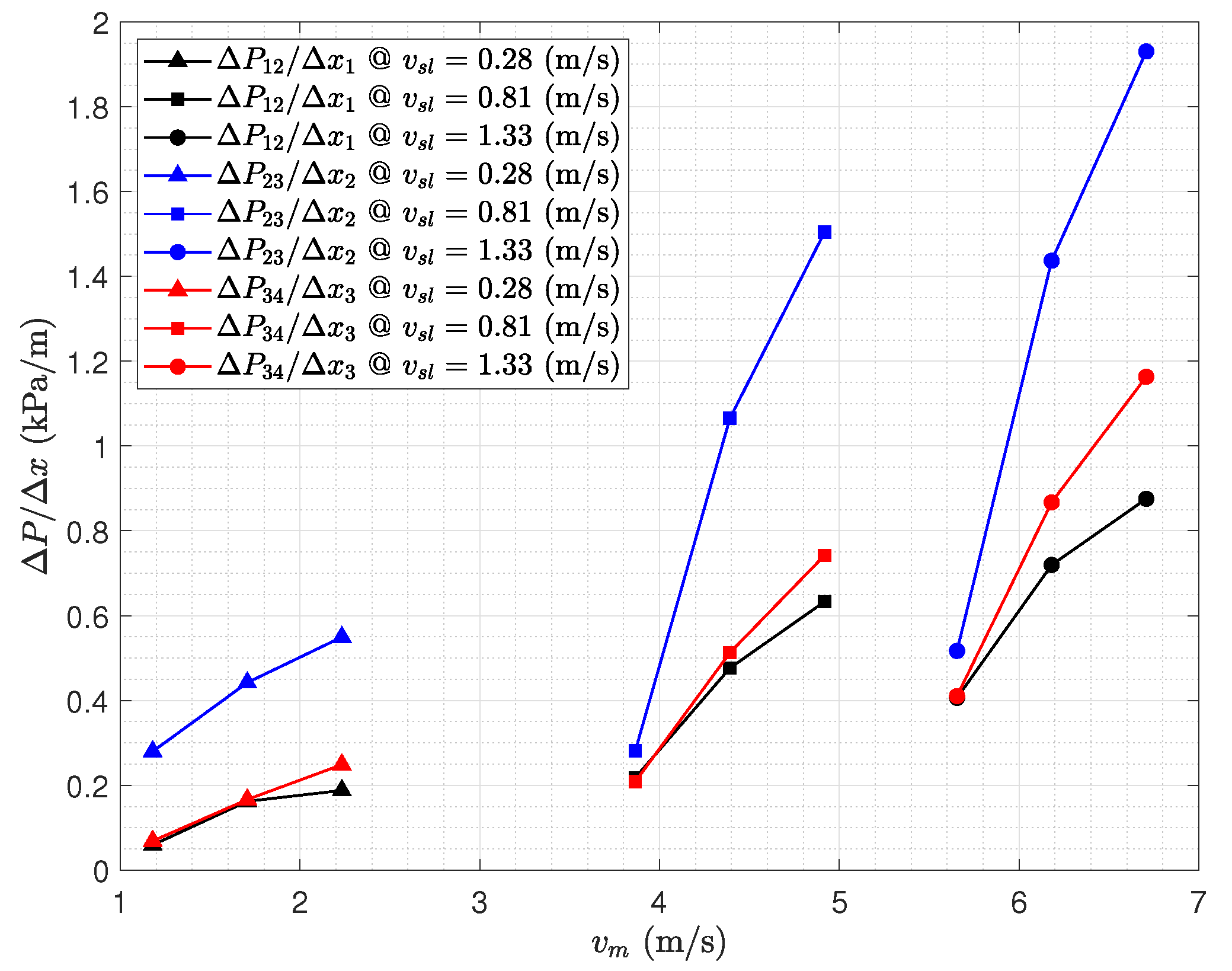
Figure 8 shows the average pressure gradients as a function of the mixture velocity, v m = v s g + v s l (where v s l = 4 Q l / ( ρ l π D 2 ) and v s g = 4 Q g / ( ρ g π D 2 ) are the superficial liquid and gas velocities). The gradients are similar for low v m values, but exhibit substantial differences at higher velocities. In the latter case, the average pressure values cease to represent good estimates because the elevated number of fluctuations produces a wider statistical dispersion. Therefore, a more meaningful measure of the pressure drop may be defined in terms of a root-mean-square (or RMS) value that takes into account the statistical dispersion. We accordingly use
Δ P i j R M S = Δ P i j ¯ 2 + σ Δ P i j 2 .
Here, Δ P i j ¯ is the arithmetic mean and σ Δ P i j is the standard deviation of the data. As can be seen in Figure 9, this estimate underlines the significance of the fluctuations with respect to the average pressure in each leg of the pipe. In 1994, Wambsganss et al. considered RMS values of the pressure drop to identify intermittent flow pattern transitions [29]. They detected an increase of the RMS pressure drop in the plug-bubble flow regime, followed by a sharp increase during the transition to the slug flow pattern. More recently, in 2002, Wang and Shoji used the RMS value to investigate the fluctuation characteristics of a two-phase flow splitting at a T-junction [30] through the analysis of the RMS differential pressures.
Since Δ P / Δ x ρ Δ v 2 / D , an analogous scaling for the high-viscosity two-phase flow can be defined as ( Δ P i j / Δ x i ) ρ m ¯ Δ v m 2 / D (with ρ m ¯ denoting the average mixture density). Thus, we write the empirical correlation
Eu i = a Q l Q g b ,
where Eu i represents the two-phase RMS Euler number of the i-th section
Eu i = ˙ Δ P i j 1 / 2 ρ m ¯ v m 2 R M S .
The regression parameters a and b can be estimated from the data set by means of the least square method. Alternatively, if the pressure gradient needs to be considered explicitly, one may recast Equation (2) in the following manner
Δ P i j Δ x i R M S = a Q l Q g b ρ m ¯ v m 2 2 D .
From the physical viewpoint, we interpret the right hand side of Equation (4) as the RMS interplay between the hydrodynamic head and the viscous losses. Thus, a serves as a kind of two-phase loss coefficient, which is weighted by some power b of the ratio Q l / Q g . The estimated numerical values of the parameters a and b are summarized in Table 10 for the indicated mixture velocity ( v m ). Figure 10 and Figure 11 show Eu i as a function of Q l / Q g .
Note in Figure 10 (for neighboring measurement ports) and Figure 11 (for distant measurement ports) that the values of the scaled pressure drop (embodied in the Eu) are, roughly, in a linear proportion to the ratio Q l / Q g . The slopes of the respective fitting curves decrease somewhat with Q l / Q g , while being shifted towards higher values of Eu. This results from complete dominance of the liquid phase on the frictional losses, an effect that can only increase as the gas flow rate is reduced. Meanwhile, the relative reduction of the slope is explained by the corresponding increase of the hydrodynamic head at higher Q l / Q g ratios.
According to Figure 10a, Eu i exhibits a near linear dependence with respect to the ratio Q l / Q g in the upstream section of the pipe. In contrast, the linear dependence is lost in the U-section, except at low mixture velocities (Figure 10b). For moderate and intermediate v m , the data are proportional to a (near) square root of Q l / Q g . In the downstream section of the pipe, we see that Eu i follows similar trends as those observed in upstream section (Figure 10c). However, the overall values of Eu i (hence of the pressure gradient) are higher in this section. Again, this is indicative of the effect produced by the slug ejection process at the outlet.
It is important to note that global estimates, produced with measurements from distant (i.e., non-adjacent) ports, tend to obscure the local effects in certain special sections of the flow system, such as the U-turn in this case. This is clearly seen by in Figure 11b,c, which incorporate the effects in the U-turn to those of the inlet and exit straight sections.

4. Conclusions

A series of high-viscosity, two-phase flow experiments were conducted in a flow loop with a length-to-diameter ratio L / D 700 . As a result of this relatively high ratio, the flow was developed for a longer time and revealed unique dynamical effects. The mixtures under consideration were produced with several mass-flow-rate combinations of air and glycerin.
The flow was statistically characterized from the time-series to analyze the pressure itself. The resulting pressure distributions showed sensitivity with respect to the flow rates, as well as to the appearance of secondary flows (in the U-section) and to the slug ejection effects. Nonetheless, the pressure drop in all three sections exhibited an almost linear dependence on the gas and liquid flow rates.
In order to adequately account for the pressure fluctuations along the pipe, the root-mean-square (or RMS) values of the pressure gradients were calculated. The corresponding plots show that some elements of the flow system (e.g., like the U-section) may have a significant impact on the local pressure drop. To estimate the RMS pressure gradient in any section of the pipe, we propose a simple correlation based on a RMS Euler number that is weighted with the ratio of the flow rates. The regression parameters are provided together with the corresponding computations for the experiments here reported.

Author Contributions

All authors contributed equally to this work. All authors have read and agreed to the published version of the manuscript.

Funding

This research received no external funding.

Acknowledgments

The authors would like to acknowledge the support from Universidad Nacional Autónoma de México (UNAM), Universidad del Norte, Scholarship Contract Identification Number: UN-OJ-2017-38125 and Minciencias (Colciencias) through Convocatoria No. 727 de 2015.

Conflicts of Interest

The authors declare no conflict of interest.

References

  1. Meyer, R.F.; Attanasi, E.D. Heavy Oil and Natural Bitumen-Strategic Petroleum Resources, Report, USGS Numbered Series. 2003. Available online: https://pubs.er.usgs.gov/publication/fs07003 (accessed on 23 November 2020).
  2. Meyer, R.; Attanasi, E.D.; Freeman, P. Heavy oil and natural bitumen resources in geological basins of the world. US Geol. Surv. 2007, 1, 1–42. [Google Scholar] [CrossRef] [Green Version]
  3. Martínez-Palou, R.; Mosqueira, M.; Zapata-Rendón, B.; Mar-Juárez, E.; Bernal-Huicochea, C.; Clavel-López, J.C.; Aburto, J. Transportation of heavy and extra-heavy crude oil by pipeline: A review. J. Pet. Sci. Eng. 2011, 1, 274–282. [Google Scholar] [CrossRef]
  4. Sorrel, S.; Speirs, J.; Bentley, R.; Miller, R.; Thompson, E. Shaping the global oil peak: A review of the evidence on field sizes, reserve growth, decline rates and depletion rates. Energy 2012, 1, 709–724. [Google Scholar] [CrossRef]
  5. Chala, G.; Sulaiman, S.; Japper-Jaafar, A. Flow start-up and transportation of waxy crude oil in pipelines: A review. J. Non-Newton. Fluid Mech. 2018, 1, 69–87. [Google Scholar] [CrossRef]
  6. Pedersen, S.; Durdevic, P.; Yang, Z. Challenges in slug modeling and control for offshore oil and gas productions: A review study. Int. J. Multiph. Flow 2017, 88, 270–284. [Google Scholar] [CrossRef]
  7. Sivakumar, P.; Sircar, A.; Deka, B.; Anumegalai, A.; Moorthi, P.; Yasvanthrajan, N. Flow improvers for assured flow of crude oil in midstream pipeline—A review. J. Pet. Sci. Eng. 2018, 1, 24–30. [Google Scholar] [CrossRef]
  8. Veritas, D.N. Fatigue design of offshore steel structures. In DNV Recommended Practice DNV-RP-C203; DET NORSKE VERITAS AS: Oslo, Norway, 2010. [Google Scholar]
  9. Wood, M.; Vetere Arellano, A.; Van Wijk, L. Corrosion related accidents in petroleum refineries. JRC Sci. Policy Rep. 2013, 1, 1–100. [Google Scholar] [CrossRef]
  10. Bordalo, S.N.; Morooka, C.K. Slug flow induced oscillations on subsea petroleum pipelines. J. Pet. Sci. Eng. 2018, 165, 535–549. [Google Scholar] [CrossRef]
  11. Thaker, J.; Banerjee, J. Influence of intermittent flow sub-patterns on erosion-corrosion in horizontal pipe. Corros. Sci. 2006, 48, 2363–2379. [Google Scholar] [CrossRef]
  12. Zhang, H.; Sarica, C.; Pereyra, E. Review of high-viscosity oil multiphase pipe flow. Energy Fuels 2012, 1, 3979–3985. [Google Scholar] [CrossRef]
  13. Bertola, V. Experimental characterization of gas–liquid intermittent subregimes by phase density function measurements. Exp. Fluids 2003, 34, 122–129. [Google Scholar] [CrossRef]
  14. Hernandez, J.; Montiel, J.; Palacio-Perez, A.; Rodríguez-Valdés, A.; Guzmán, J. Horizontal Evolution of Intermittent Gas-Liquid Flows With Highly Viscous Phases. In Multiphase Flow: Theory and Applications; Witpress: Southampton, UK, 2018; p. 157. [Google Scholar] [CrossRef] [Green Version]
  15. Gokcal, B.; Wang, Q.; Zhang, H.Q.; Sarica, C. Effects of high oil viscosity on oil/gas flow behavior in horizontal pipes. SPE Proj. Facil. Constr. 2008, 3, 1–11. [Google Scholar] [CrossRef]
  16. Gokcal, B. An Experimental and Theoretical Investigation of Slug Flow for High Oil Viscosity in Horizontal Pipes. Ph.D. Thesis, University of Tulsa, Tulsa, OK, USA, 2008. [Google Scholar]
  17. Brito, R. Effect of Medium Oil Viscosity on Two-Phase Oil-Gas Flow Behavior in Horizontal Pipes. Ph.D. Thesis, University of Tulsa, Tulsa, OK, USA, 2012. [Google Scholar]
  18. Hernández, J.; Galaviz, D.; Torres, L.; Palacio-Perez, A.; Rodríguez-Valdés, A.; Guzmán, J. Evolution of High-Viscosity Gas–Liquid Flows as Viewed Through a Detrended Fluctuation Characterization. Processes 2019, 7, 822. [Google Scholar] [CrossRef] [Green Version]
  19. Archibong-Eso, A.; Okeke, N.; Baba, Y.; Aliyu, A.; Lao, L.; Yeung, H. Estimating slug liquid holdup in high viscosity oil-gas two-phase flow. Flow Meas. Instrum. 2019, 65, 22–32. [Google Scholar] [CrossRef] [Green Version]
  20. Baba, Y.D.; Aliyu, A.M.; Archibong, A.E.; Abdulkadir, M.; Lao, L.; Yeung, H. Slug length for high viscosity oil-gas flow in horizontal pipes: Experiments and prediction. J. Pet. Sci. Eng. 2018, 165, 397–411. [Google Scholar] [CrossRef]
  21. Bendiksen, K.H.; Langsholt, M.; Liu, L. An experimental investigation of the motion of long bubbles in high viscosity slug flow in horizontal pipes. Int. J. Multiph. Flow 2018, 104, 60–73. [Google Scholar] [CrossRef]
  22. Baba, Y.D.; Archibong, A.E.; Aliyu, A.M.; Ameen, A.I. Slug frequency in high viscosity oil-gas two-phase flow: Experiment and prediction. Flow Meas. Instrum. 2017, 54, 109–123. [Google Scholar]
  23. Ekinci, S.; Aydin, T.; Sarica, C.; Pereyra, E.; Kim, T. Pipe inclination effects on slug flow characteristics of high viscosity oil-gas two-phase flow for near horizontal pipes. In Proceedings of the ASME 2017 Fluids Engineering Division Summer Meeting, Waikoloa, HI, USA, 30 July–3 August 2017; Volume 1, pp. 1–11. [Google Scholar]
  24. Al-Safran, E.; Kora, C.; Sarica, C. Prediction of slug liquid holdup in high viscosity liquid and gas two-phase flow in horizontal pipes. J. Pet. Sci. Eng. 2015, 1, 566–575. [Google Scholar]
  25. Farsetti, S.; Farisé, S.; Poesio, P. Experimental investigation of high viscosity oil-air intermittent flow. Exp. Therm. Fluid Sci. 2014, 1, 285–292. [Google Scholar] [CrossRef]
  26. Matsubara, H.; Naito, K. Effect of liquid viscosity on flow patterns of gas-liquid two-phase flow in a horizontal pipe. Int. J. Multiph. Flow 2011, 1, 1277–1281. [Google Scholar]
  27. Akagwa, K.; Hamaguchi, H.; Sakaguchi, T.; Ikari, T. Studies on the Fluctuation of pressure Drop in Two-Phase Slug Flow: 1st Report, Experimental Study. Bull. JSME 1971, 14, 447–454. [Google Scholar] [CrossRef]
  28. Al-Sarkhi, A.; Sarica, C. Power-law correlation for two-phase pressure drop of gas/liquid flows in horizontal pipelines. SPE Proj. Facil. Constr. 2010, 5, 176–182. [Google Scholar] [CrossRef]
  29. Wambsganss, M.; Jendrzejczyk, J.; France, D. Determination and characteristics of the transition to two-phase slug flow in small horizontal channels. J. Fluids Eng. 1994, 116, 140–146. [Google Scholar] [CrossRef]
  30. Wang, S.; Shoji, M. Fluctuation characteristics of two-phase flow splitting at a vertical impacting T-junction. Int. J. Multiph. Flow 2002, 28, 2007–2016. [Google Scholar] [CrossRef]
1.
API gravity is defined by the American Petroleum Institute as a measure of density that, compared to water at equal temperatures, indicates how heavy or light an oil is. Oils with API values greater than 10 are lighter than water.
2.
The root-mean-square (frequently called the quadratic mean) is the arithmetic mean of the squares of a set of values of a discrete distribution.
Figure 1. Two-phase flow loop and related equipment.
Jmse 08 01000 g001
Figure 2. Diagram of the setup. The locations of the pressure transducers and the thermocouples are labeled as P1, P2, P3, and P4. The system’s main components are the progressive cavity pump (a), the air compressor (b), the test section (c), the flow control and Coriolis devices (d), and the separator tanks (e).
Jmse 08 01000 g002
Figure 3. Gas entrainment and liquid film behavior in the high-viscosity regime (the mixture’s viscosity was slightly reduced to μ 0.5 Pa s (500 cP) to enhance the visualization).
Jmse 08 01000 g003
Figure 4. Histograms of Δ P 12 , Δ P 23 , Δ P 34 for a liquid mass flow rate 1.3 kg/s with 0.005, 0.02, and 0.03 kg/s of gas mass flow rate. Data from two experiments are presented.
Jmse 08 01000 g004
Figure 5. Histograms of Δ P 12 , Δ P 23 , Δ P 34 for a liquid mass flow rate 3.7 kg/s with 0.005, 0.02, and 0.03 kg/s of gas mass flow rate. Data from two experiments are presented.
Jmse 08 01000 g005
Figure 6. Histograms of Δ P 12 , Δ P 23 , Δ P 34 for a liquid mass flow rate 6.1 kg/s with 0.005, 0.02, and 0.03 kg/s of gas mass flow rate. Data from two experiments are presented.
Jmse 08 01000 g006
Figure 7. Average pressure drop computed with the data from the set of experiment A.
Jmse 08 01000 g007
Figure 8. Mean pressure gradients.
Jmse 08 01000 g008
Figure 9. RMS pressure gradients.
Jmse 08 01000 g009
Figure 10. Predictions for the Euler number obtained with Equation (4) and the data set of experiment B. Respectively, image (a) corresponds to the first column in Table 10, (b) corresponds to the second column, and (c) to the third column.
Jmse 08 01000 g010
Figure 11. Predictions for the Euler number obtained with Equation (4) and the data set of experiment B. Respectively, image (a) corresponds to the first column in Table 11, (b) corresponds to the second column, and (c) to the third column.
Jmse 08 01000 g011
Table 1. Liquid and gas mass-flow-rates ( Q l and Q g in kg/s) and superficial velocities ( v s l and v s g in m/s). v s g varied within the indicated maximum and minimum values.
Q l v sl Q g v sg
maxmin
1.30.230.0050.990.73
3.70.680.023.982.93
6.11.110.035.984.40
Table 2. Symbology for the length and pressure drop in each test section’s leg.
ItemDefinitionValueUnits
Δ x 1 x P 2 x P 1 18m
Δ x 2 x P 3 x P 2 4
Δ x 3 x P 4 x P 3 21
Δ P 12 P 1 P 2 -Pa
Δ P 23 P 2 P 3 -
Δ P 34 P 3 P 4 -
Table 3. Mean pressure drops (in kPa) for pipeline sections 1, 2 and 3, in terms of Q l and Q g (in kg/s).
Δ P 12 Δ P 23 Δ P 34
Q l / Q g 0.0050.020.030.0050.020.030.0050.020.03
1.30.751.882.210.400.50.71.192.433.66
3.73.857.659.560.862.092.844.309.7713.46
6.17.2812.4414.911.983.9858.5917.623.3
Table 4. Normalized mean pressure drop in pipeline sections 1, 2 and 3, in terms of Q l and Q g (in kg/s).
Δ P 12 * Δ P 23 * Δ P 34 *
Q l / Q g 0.0050.020.030.0050.020.030.0050.020.03
1.30.050.130.150.080.100.140.050.100.16
3.70.260.510.640.170.420.570.180.420.58
6.10.490.831.000.400.801.000.370.761.00
Table 5. Standard deviation (in kPa) in terms of Q l and Q g (in kg/s).
σ Δ P 12 σ Δ P 23 σ Δ P 34
Q l / Q g 0.0050.020.030.0050.020.030.0050.020.03
1.30.762.242.561.051.702.090.812.523.73
3.70.723.886.190.733.715.310.854.547.86
6.10.683.635.090.604.155.890.794.677.33
Table 6. Kurtosis in terms of Q l and Q g (in kg/s).
κ Δ P 12 κ Δ P 23 κ Δ P 34
Q l / Q g 0.0050.020.030.0050.020.030.0050.020.03
1.33.265.8112.976.4811.5922.273.193.14.54
3.72.862.73.632.734.046.032.752.842.03
6.12.912.642.753.042.082.363.032.662.37
Table 7. Skewness in terms of Q l and Q g (in kg/s).
ζ Δ P 12 ζ Δ P 23 ζ Δ P 34
Q l / Q g 0.0050.020.030.0050.020.030.0050.020.03
1.30.521.82.982.122.914.050.581.081.48
3.70.070.090.560.331.471.860.37−0.05−0.14
6.10.18−0.03−0.03−0.030.570.75−0.040.270.13
Table 8. Pressure gradients along Δ x 1 and Δ x 3 , in terms of Q l and Q g (in kg/s), for experiment A.
Q g 0.0050.020.03
Q l Δ P 12 / Δ x 1 Δ P 34 / Δ x 3 Δ P 12 / Δ x 1 Δ P 34 / Δ x 3 Δ P 12 / Δ x 1 Δ P 34 / Δ x 3
1.30.040.060.10.120.120.17
3.70.210.20.420.470.530.64
6.10.40.410.690.840.831.11
Table 9. Pressure gradients along Δ x 1 and Δ x 3 , in terms of Q l and Q g (in kg/s), for experiment B.
Q g 0.0050.020.03
Q l Δ P 12 / Δ x 1 Δ P 34 / Δ x 3 Δ P 12 / Δ x 1 Δ P 34 / Δ x 3 Δ P 12 / Δ x 1 Δ P 34 / Δ x 3
1.30.040.060.110.120.130.17
3.70.210.20.420.460.520.64
6.10.410.410.690.840.831.1
Table 10. Regression parameters for the RMS Euler numbers at a given v s l (from the data set of experiment B).
v sl (m/s)Eu 12 Eu 23 Eu 34
0.2376 (m/s) a = 2.313 × 10 5 a = 1.093 × 10 5 a = 2.756 × 10 5
b = 1 b = 1.4 b = 1
0.6761 (m/s) a = 2.926 × 10 5 a = 4.018 × 10 4 a = 6.088 × 10 5
b = 0.9 b = 0.55 b = 0.78
1.1147 (m/s) a = 3.072 × 10 5 a = 0.3.265 × 10 4 a = 6.378 × 10 5
b = 0.85 b = 0.55 b = 0.75
Table 11. Regression parameters for the RMS Euler numbers at a given v s l (from the data set of experiment B).
v sl (m/s)Eu 14 Eu 13 Eu 24
0.2376 (m/s) a = 7.603 × 10 6 a = 8.806 × 10 6 a = 9.698 × 10 6
b = 1.2 b = 1.2 b = 1.2
0.6761 (m/s) a = 2.822 × 10 5 a = 2.625 × 10 5 a = 5.384 × 10 5
b = 0.9 b = 0.9 b = 0.8
1.1147 (m/s) a = 4.49 × 10 5 a = 3.194 × 10 5 a = 6.547 × 10 5
b = 0.8 b = 0.85 b = 0.75
Publisher’s Note: MDPI stays neutral with regard to jurisdictional claims in published maps and institutional affiliations.