Modeling Impact of Intertidal Foreshore Evolution on Gravel Barrier Erosion and Wave Runup with XBeach-X


1
National Oceanography Centre, 6 Brownlow St., Liverpool L3 5DA, UK
2
Department of Geography and Planning, University of Liverpool, Roxby Building, Chatham St, Liverpool L69 7ZT, UK
*
Author to whom correspondence should be addressed.
J. Mar. Sci. Eng. 2020, 8(11), 914; https://doi.org/10.3390/jmse8110914
Submission received: 5 October 2020
/
Revised: 7 November 2020
/
Accepted: 10 November 2020
/
Published: 12 November 2020
(This article belongs to the Special Issue Observation, Analysis, and Modeling of Nearshore Dynamics)
Abstract
:This paper provides a sensitivity analysis around how characterizing sandy, intertidal foreshore evolution in XBeach-X impacts on wave runup and morphological change of a vulnerable, composite gravel beach. The study is motivated by a need for confidence in storm-impact modeling outputs to inform coastal management policy for composite beaches worldwide. First, the model is run with the sandy settings applied to capture changes in the intertidal foreshore, with the gravel barrier assigned as a non-erodible surface. Model runs were then repeated with the gravel settings applied to obtain wave runup and erosion of the barrier crest, updating the intertidal foreshore from the previous model outputs every 5, 10 and 15 min, and comparing this with a temporally static foreshore. Results show that the scenario with no foreshore evolution led to the highest wave runup and barrier erosion. The applied foreshore evolution setting update is shown to be a large control on the distribution of freeboard values indicative of overwash hazard and barrier erosion by causing an increase (with 5 min foreshore updates applied) or a decrease (with no applied foreshore updating) in the Iribarren number. Therefore, the sandy, intertidal component should not be neglected in gravel barrier modeling applications given the risk of over- or under-predicting the wave runup and barrier erosion.
1. Introduction
Gravel barrier coasts, found worldwide on high-latitude, previously glaciated coasts (Northern Europe, Japan, U.S.A.) can experience erosion and overtopping during high-energy storm events, resulting in financial and societal losses and fatalities [1]. These coastlines are becoming increasingly vulnerable as wave climates become modified by changing storm tracks [2] and as sea-level rise acts to shorten the return period of a given extreme water level and increase the frequency of coastal flooding [3]. In the U.K., where gravel beaches and gravel barrier coasts account for 1000 km of coastline, gravel has been used to nourish some coastlines to maintain the natural protection they afford [4].
Barrier beaches are dynamic systems which evolve according to multiple factors over various time-scales. In the short and medium term, barriers are affected by the local wave climate and episodically when wave runup exceeding the barrier crest allows the mobilization of sediments onto the barrier crest and back barrier (overwash), inundation and in extreme scenarios, barrier breaching [5]. These events are likely to pose a hazard to hinterland communities, which will face an amplified risk of barrier breaching and overwash from future sea-level rise [3]. Their long-term (decadal to centennial) evolution and survival is controlled by the rate of relative sea-level rise, sediment size, sediment supply rates, accommodation space and local topography [6,7]. Insights into the long-term evolution of barriers provide critical information on the underlying drivers of coastal barrier response.
Jennings and Shulmeister [8] provide a field-based classification scheme for gravel beaches, with the key determinant variables being beach slope, Iribarren number, average grain size and berm height. Their study divides gravel beaches into three classifications:
- Pure gravel beaches: Steep slopes () = 0.08–0.24, with average sediment size decreasing from the storm berm down to the swash zone.
- Mixed sand–gravel (MSG): Moderate slopes () = 0.04–0.13, subdivided into beaches with (a) largely intermixed sand and gravel and (b) a higher degree of sorting of sand and gravel in a cross-shore direction.
- Composite beaches: A steep gravel berm with a low-angle intertidal foreshore and well-sorted sand and gravel in the cross-shore direction. Slope values are similar to that of MSG beaches.
Sandy beaches also act as a natural coastal defense, providing the rationale for the development of the XBeach-X model used in this study [9]. Hence event-driven evolution of the low-angle, sandy, intertidal foreshore of a composite gravel beach is also an important consideration, particularly as sea-level rise acts to amplify beach erosion (e.g., [10]). Changes in beach morphology over the time-scales of individual storm events are shown to be an important control on wave overwash volume [11], as are seasonality and antecedent conditions [12]. These factors also control barrier response in addition to the described long-term factors.
Historically, understanding the controls on the evolution of gravel beaches and barriers during storm events lagged behind sandy systems. However, recent developments have included the development of numerical models for gravel coasts at mesoscales [13] and the parameterization of wave runup from beach slope and wave conditions for a gravel coast [14]. The previously used general equation for runup on sandy beaches developed by Stockdon et al. [15] was shown in Poate et al. [14] to underpredict (2 exceedance wave runup) by up to 50% when applied to gravel coasts with energetic conditions. Sallenger Jr [16] categorized the morphologic response of barrier islands according to decreasing levels of freeboard:
- Swash Regime: where wave runup acts on the foreshore without impacting the dune.
- Collision Regime: where exceeds the dune toe. Eroded material is transported off- or alongshore but unlike the swash regime does not return to replenish the barrier.
- Overwash Regime: where exceeds the berm crest, leading to erosion of the dune and deposition inland.
- Inundation Regime: where the barrier becomes completely submerged by a high value and the flows are no longer overwash.
Further work by Plomaritis et al. [17] developed this classification into a regional scale assessment of storm related overwash and barrier breaching using a numerical model of coastal overwash [18], allowing the formulation of overwash volumes without the need for numerical modeling which is computationally expensive over larger spatial scales. Recent literature has begun to study mixed sand–gravel beaches under different tectonic settings [19], and where gradients in both alongshore and cross-shore sediment transport play a role in governing the sediment transport regime [20,21,22].
Previous work carried out prior to the development of the XBeach-G extension by McCall et al. [13,23] used a composite gravel beach on the south coast of the U.K. as a validation site [24]. Here, the modifications made to the model did not (and were not intended to) capture the evolution of the sandy, intertidal terrace. When XBeach-G was introduced with specific morphodynamics for applications to pure gravel beaches in McCall et al. [23], it was applied to a swash-aligned composite beach similar to that of the study area, Newgale. Although Masselink et al. [25] state that XBeach-G can compute wave transformation and runup for MSG and composite gravel beaches with reasonable accuracy, it lacks a solution for suspended sediment transport and hence is limited in its morphodynamic capabilities for those types of gravel beaches.
In this paper, we carry out a sensitivity analysis around how the distribution of freeboard values and morphologic response of a swash-aligned composite beach varies in response to the method used to characterize the foreshore evolution within the storm-impact model. Our aim is to provide insights into how the model outputs are influenced by the foreshore characterization, approaching this from a modeling context rather than a geomorphic investigation of barrier behavior. The work aims to address deficiencies in modeling composite barrier settings, as the model used XBeach-X can use multiple sediment fractions but cannot currently apply spatially varied sand and gravel settings to different parts of its domain. The inherent differences in the hydrodynamics of the sand and gravel components, such as infiltration, and in the morphodynamics, such as the potential of a gravel barrier to slump when the angle of repose is exceeded, demands applying the two model settings to their respective components. Insights into the feedback between the evolution of the sandy, intertidal terrace and gravel barrier components of a composite beach is of importance for shoreline management and to inform design standards and strategies on vulnerable composite beaches worldwide, where overwash and inundation regimes threaten key infrastructure.
2. Study Site: Newgale, U.K.
The beach at Newgale in the northwest corner of St Bride’s Bay, Pembrokeshire, U.K. (Figure 1) can be characterized as a composite gravel beach with an approximate slope of = 0.1, falling within the range of values identified for these systems. The area is macrotidal with a mean tidal range of (measured at Milford Haven tide gauge), and is exposed to both locally generated wind waves in addition to North Atlantic swell. Wave transformation modeling carried out by Royal Haskoning DHV [26] demonstrates that the waves with more extreme significant wave height () and peak period () values are typically south-westerly in origin, strongly aligned with the local shoreline orientation of this area of St Bride’s Bay. The composite gravel beach at Newgale formed from paraglacial, offshore sediments, transported onshore during Holocene sea-level transgression. This is characteristic of a macrotidal, wave-dominated coast at mid to high latitude, and as is common with swash-aligned barriers, there is no long-term addition of sediment from offshore or adjacent sources. The mouth of the Brandy Brook is at the northern end of the frontage (Figure 1), and the channel is kept free of sediment to allow drainage. Most properties in the village lie off the coastal floodplain to the north, where the managed realignment policy intends to protect the village. However a campsite, a public house and the road connecting Newgale to the rest of Pembrokeshire are vulnerable to inundation if the gravel barrier fails, and the shoreline management policy for this area moves towards no active intervention in 50 to 100 years (Table 1).
The gravel barrier at Newgale suffers from overwashing of sediments on to the road, and its behavior and vulnerability has been studied for operational purposes since the early 1990s. Under extreme conditions, the gravel barrier can be breached, leading to extensive inundation of the low-lying hinterland and prolonged road closure. This occurred most recently in December 2013 and January 2014 (Figure 1), and analysis from tide gauge records at Milford Haven indicated that the water level had a return period in the order of 1:20 to 1:25 years. The current management strategy for the gravel barrier is to accept periodic overwash or failure and to maintain 4 m to 5 m beach width at the crest. The barrier is then reprofiled to this criterion when overwash during storms leads to sedimentation on the road and hinterland. Under sea-level rise, total failure of the gravel barrier could be expected annually [26]. A recent study commissioned by the Pembrokeshire Council (responsible for coastal defense and infrastructure) concludes that this management strategy is likely to become unsustainable over a period of 10–20 years as the gravel barrier continues to deteriorate. At this point, the risk of the gravel barrier breaching, and associated closure and maintenance costs will become unacceptably high. The site therefore provides an appropriate case study for numerical modeling of the morphologic response of the gravel barrier (and the sandy foreshore on which it resides) to storm conditions, since the barrier is shown to be vulnerable to water levels of approximately 1:20 year return periods and long period swell waves, shown to cause more wave overtopping for gravel coasts than wind waves [31].
3. Modeling Approach
3.1. Storm-Impact Model: XBeach-X
XBeach-X is an open source, process-based hydrodynamic model aimed at simulating coastal change over time-scales in the order of individual storm events up to spatial scales of kilometers. The model was introduced by Roelvink et al. [9] in response to the 2004 and 2005 hurricane seasons in the U.S.A. Since then, it has been extensively used and validated in a variety of coastal settings, including saltmarshes [32,33], sandy, barrier coasts [5,34], sandy coasts defended by hard engineering structures [11] and coral reefs [35,36]. Early efforts to apply XBeach to gravel settings were made by Jamal et al. [24] and Williams et al. [37] but do not explicitly resolve wave runup from incident waves. Subsequent developments for gravel applications were the addition of a depth-averaged non-hydrostatic extension in XBeach-G (a standalone version for applications to gravel coasts, and ported into the XBeach-X release version) allowed for the solution of wave by wave flow due to short waves in shallow water depths, a process of greater importance on steeper gravel beaches due to incident waves dominating over waves of infragravity frequencies [23]. XBeach-G includes a solution for groundwater exchange between the surface and sub-surface, but currently resolves wave propagation, sediment transport and overwash in the cross-shore dimension only. It is shown to make good predictions of wave transformation and runup. Alongshore sediment transport for a Mediterranean mixed sand–gravel beach has been parameterized in XBeach-G by calculating a flux using the Van Rijn [38] equation and redistributing the flux in the cross-shore dimension [20]. Currently XBeach-G does not resolve alongshore sediment transport, and nor is there the capability to spatially vary the sand/gravel settings across the model domain.
In this study, the focus is on cross-shore processes as regional wave modeling carried out by Royal Haskoning DHV shows that the waves are strongly aligned with the shoreline orientation, and that gradients in alongshore sediment transport are shown to be negligible [26]. Therefore, resolving only cross-shore processes in both sandy and gravel model settings is acceptable for this site. Here, XBeach-X is run in the non-hydrostatic mode for both the sand and gravel simulations, resolving the propagation and decay of all individual waves and associated processes including wave-induced setup, currents, infragravity and short period waves.
3.2. Wave and Water Level Boundary Conditions
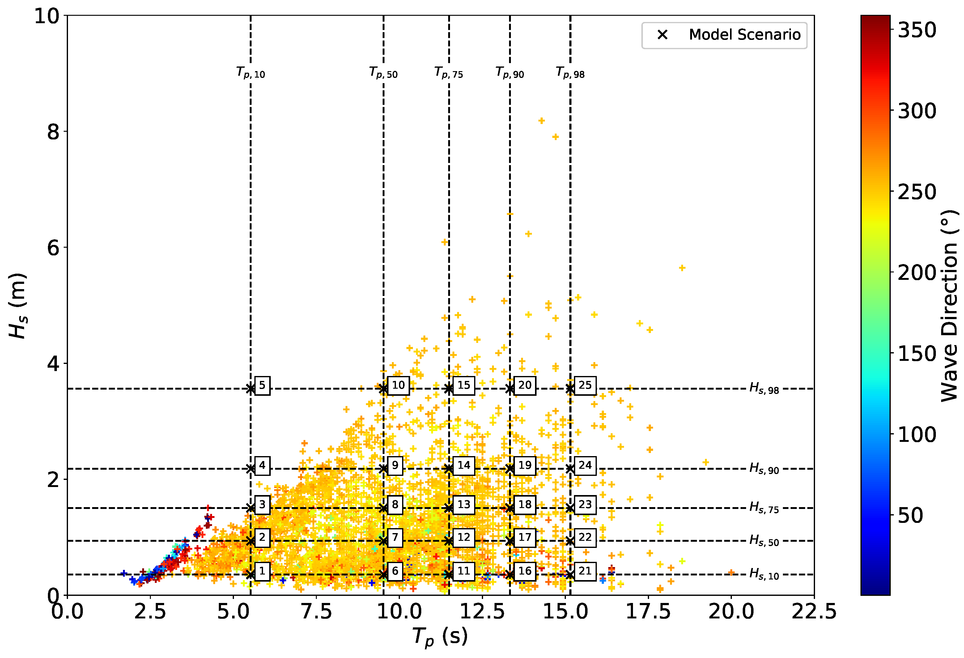
To address the research questions for this paper, representative and were generated using percentile values from modeled data (e.g., [39]), instead of using events represented by a given probability (e.g., [11,31]). Firstly, each high water from the Milford Haven tide gauge (see Figure 2) is identified over the entire range of available data (1980 to 2018). At each of the identified high waters, U.K. Met Office WaveWatchIII data [40] was then used to provide the corresponding and values. The 10th, 50th, 75th, 90th and 98th percentiles of and at high water were then calculated, along with the average amount of time per year the percentile values are exceeded in the WaveWatchIII dataset (Figure 3 and Table 2).
These and percentiles, along with a single shore-normal wave direction form the wave forcing for XBeach-X. These conditions are forced using a unimodal JONSWAP spectrum provided by XBeach-X, with the default settings for the spectrum’s peak enhancement factor (3.3, the mean factor provided in [41]) and directional spreading coefficient (10) applied. This value is consistent with average directional spreading for the area (24 ), derived from the WaveWatchIII model data.
Scenarios 1 to 25 in Table 2 are used to force XBeach-X with the Highest Astronomical Tide (HAT, Figure 4). The Proudman Oceanographic Laboratory Tidal Prediction Software (POLTIPS3 [42]) was used to find the relevant HAT tidal cycle at Milford Haven, which occurred on 29 September 2015 at a level of m above Ordnance.Datum.Newlyn.(m ODN) according to National Tidal and Sea Level Facility [43].
3.3. Cross-Shore Profile
Given that the gravel barrier at Newgale is strongly swash-aligned, and that XBeach-G does not resolve alongshore sediment transport, a one-dimensional modeling approach is used. A single cross-shore profile, reflecting the shoreline management policy of maintaining 4 width above 7 m ODN, is taken from 1 m resolution Light Detection and Ranging (LiDAR, Figure 5), the finest resolution that was available (downloaded from the Natural Resources Wales database [44]). These surveys are the responsibility of the local authority and, as with the LiDAR survey used here, are not routinely scheduled at low spring tides when the maximum area of foreshore is exposed. In order to extend the transect offshore to the closure depth (calculated to be −17 m ODN using the equation provided by Hallermeier [45]), 1 arcsecond resolution bathymetry is taken from EDINA Digimap’s marine database [46] and corrected to the same vertical datum. Interpolation has been used to ensure a more realistic transition between the two applied datasets. Deltares provides a toolbox for the model [47], which was used to ensure that sufficient grid points per wavelength were interpolated to ensure the model remains stable. Here, 60 points per wavelength are used, based on the minimum applied value (Table 2).
3.4. Updating the Profile with Foreshore Evolution
The profile is divided into sandy, intertidal foreshore and gravel barrier components and modeled as separate systems with uniform sediment in each component. The toe of the gravel barrier ( m ODN) is used as a threshold to partition the sandy, intertidal foreshore and the gravel barrier. XBeach-X was first run with the sandy settings enabled on the foreshore only for each percentile combination for a single tidal cycle (Table 2). In these model runs, the gravel barrier is assigned as non-erodible, so that only the foreshore is allowed to morphologically evolve. Water levels and bed profiles (zs and zb in XBeach-X) are saved at 60 intervals.
Each percentile combination is then repeated with the model’s gravel settings enabled, this time with the sandy foreshore assigned as a non-erodible surface. The use of the useXBeachGsettings parameter is activated to apply the XBeach-X gravel settings. Additionally, the following settings were set such that the XBeach-X setup is more appropriate for the hydrodynamics and morphodynamics of gravel beaches:
- The applied gravel grain sizes were set to = and = .
- The porosity factor was set to 0.45.
- The model’s white-colebrook-grainsize parameter was enabled, instructing the model to derive a bed friction coefficient based on the applied .
- The model’s groundwater exchange mechanism was enabled (gwflow).
It is assumed that any on-shore transport of sand onto the gravel barrier has a negligible impact on its morphology given the applied gravel grain sizes and porosity factors (provided above) are unlikely to allow substantial sedimentation of sand on a gravel barrier during a storm. The scenarios used to update the sandy foreshore evolution within the gravel model runs are described in Table 3.
When the model reaches a time to morphologically update the foreshore, the water level and bed profile for the relevant time are identified in the model outputs of foreshore evolution. The new cross-shore transect for the next model run then consists of the updated foreshore (using the model outputs from the sandy settings) for points offshore from the barrier toe combined with gravel that has slumped onto the foreshore (if applicable), and the updated gravel barrier for the points onshore from and including the barrier toe. The amount of sediment available at each gravel grid point is also updated according to the sedimentation or erosion of the gravel barrier during the time period, allowing the model to mobilize gravel sediment which has been transported offshore. The model then resumes using the water level at each grid point and repeats the morphological updating according to the given scenario until the water level recedes below the toe of the barrier on the ebb tide. The JONSWAP spectrum remains the same across each model run to ensure consistency in the wave field.
4. Results
This section explores the results of the XBeach-X modeling of the and percentile combinations under each of the foreshore evolution settings described in Section 3.4 (S1 to S5). Results using values of and which are less than the 75th percentile are not shown, as the values induced no (or negligible) erosion of the barrier. The following proxies are used to show the influence of the foreshore evolution setting on wave runup and morphological response of the gravel barrier (visualized in Figure 6):
- Freeboard: Calculated as the difference in elevation between the barrier crest and at intervals when the water level exceeds the toe of the barrier ( m ODN). is calculated using the runup gauge output function in XBeach-X. Freeboard values are set to zero when exceeds the barrier crest. The calculation of freeboard accounts for any lowering of the barrier crest throughout the simulation, whereas using alone would neglect this.
- Relative wave runup (), where is one-minute averaged.
- Elevation change of the managed barrier crest (): Calculated by integrating cumulative elevation change across the cross-shore area equal to or above 7 m ODN (the height at which the management policy dictates that 4 to 5 barrier width should be maintained) at one-minute intervals. The morphologic response enters the overwash regime as begins to rival the barrier crest.
- Elevation change of the barrier crest (): One-minute averaged change of the maximum height of the barrier.
- Elevation change of the barrier toe (): Calculated by integrating cumulative elevation change across the cross-shore area between the barrier toe and 5 offshore of the barrier toe at one-minute intervals
- Back-barrier sedimentation (): Calculated by integrating cumulative elevation change across the area between the base of the back barrier and the landwards boundary of the model at one-minute intervals.
- Iribarren Number (, [48]) to determine the type of breaking wave: Calculated using Equation (1):where is the deep water wavelength, g = / and is the beach slope (area between the barrier crest (x = 0 ) and the grid cell which experiences the deepest scour (x = ). Values >3.3 represent surging/collapsing waves and values <3.3 represent plunging waves. The spilling wave regime, characterized by values of < 0.5 are not shown to occur due to the steep nature of the beach.
4.1. Freeboard and Relative Wave Runup under Applied Foreshore Evolution Settings
Figure 7 demonstrates that S1 (no updating of foreshore) causes the most freeboard values which pose an overwash hazard, followed by S2, where the foreshore is only updated when the water level reaches the barrier on the flood and ebb tides. S3, which has the most frequent foreshore updating has the highest freeboard values (lowest overwash hazard), where the highest probability density of freeboard values are found between 2.5 to 4.5. Across the and percentile combinations, there is negligible difference in the frequency of hazardous freeboard values between S4 and S5 (10 and 15 min foreshore updates, respectively), but values under these settings are consistently between S1–S2 and S3. For freeboard values close to zero under the most extreme percentile combinations, there is a substantial difference between S1–S2, where the freeboard distribution is dominated by values <1 and those values of S3–S5 where the foreshore is being updated while the water level exceeds the toe of the barrier. Under the and conditions, the probability density of the most hazardous freeboard values under S1 and S2 is a factor of 30 higher compared to S3 and a factor of 5 when compared with S4 and S5.
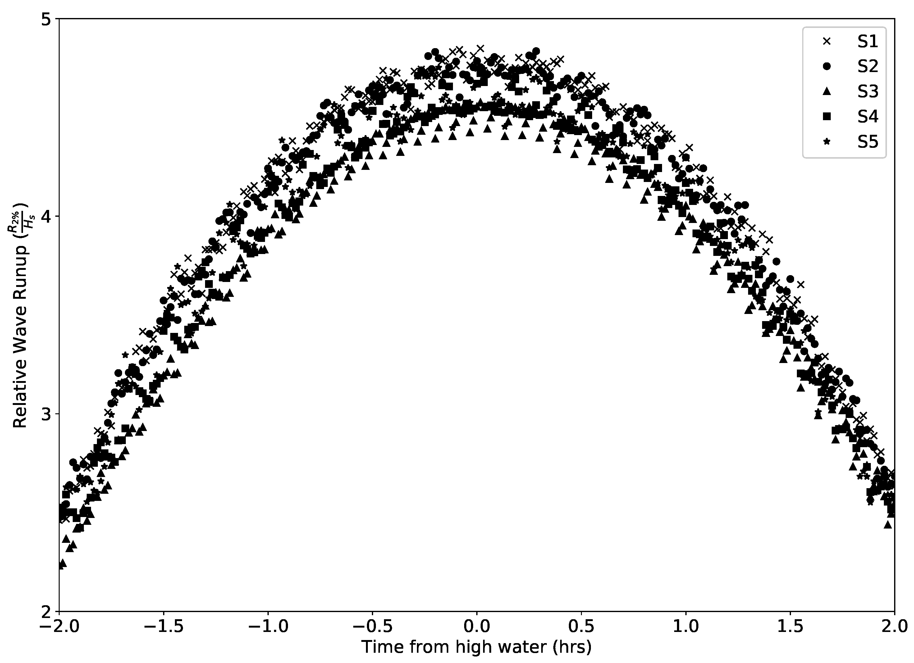
Figure 8 demonstrates the overall sensitivity of to averaged across each and percentile combination for S1 to S5. It shows that S3 consistently shows the lowest relative wave runup values throughout the high-water window. S1 exhibits the highest relative wave runup compared to the other sand and gravel settings for 58% of the observations in the time series, followed by S2 with 35%. For S3–S5, where there is updating of the foreshore evolution while the water level exceeds the toe of the barrier, there are fewer points in time where these settings show the highest relative wave runup. The number of observations of each setting exhibiting the highest relative wave runup shows an increase from 0% for S3 to % for S4 and % for S5, an exponential increase as the frequency at which foreshore evolution is updated decreases. Calculating time-integrated relative wave runup for each of the applied foreshore settings demonstrates negligible difference between S1 and S2 (<%), increasing to 7% between S1 and S3, the extremes of the applied foreshore evolution settings, with no and 5 min foreshore evolution updates, respectively.
4.2. Barrier Change under Applied Foreshore Evolution Settings
Figure 9 shows negligible barrier erosion begins to occur under and with S1 and S2 applied. Barrier erosion under S3–S5 with the more frequent foreshore evolution updating only occurs under the most extreme condition (98th percentile). There are substantial differences in elevation change of both the barrier crest and back barrier under S1–S2 and S3–S5 (Table 4), consistent with the difference in the distribution of freeboard values shown in Figure 7. The foreshore evolution setting is also shown to exercise some control on the timing of the onset of barrier erosion. For the most extreme applied wave condition ( and ), erosion of the barrier crest is shown to begin around 45 prior to high water under S1. This contrasts with S4 and S5, where erosion of the barrier crest commences around 20 min before high water.
The impact of the foreshore evolution setting on the cross-shore sediment transport is also reflected by differences in the degrees of sedimentation of gravel on the landward side during overwash regime. Table 4 shows an order of magnitude difference between S1–S2 and S3–S5 for both mean barrier erosion and mean back-barrier sedimentation when averaged across each and scenario. Figure 10 confirms the trends shown in erosion of the barrier crest. Even under the most extreme modeled wave conditions, S3 is not shown to be capable of causing the barrier to overwash given the small magnitude of crest erosion. As with the barrier erosion, there is also variability in the onset of sedimentation at the base of the back barrier. For the - scenario, there is shown to be approximately a 15 difference between S1–S2 and S4–S5.
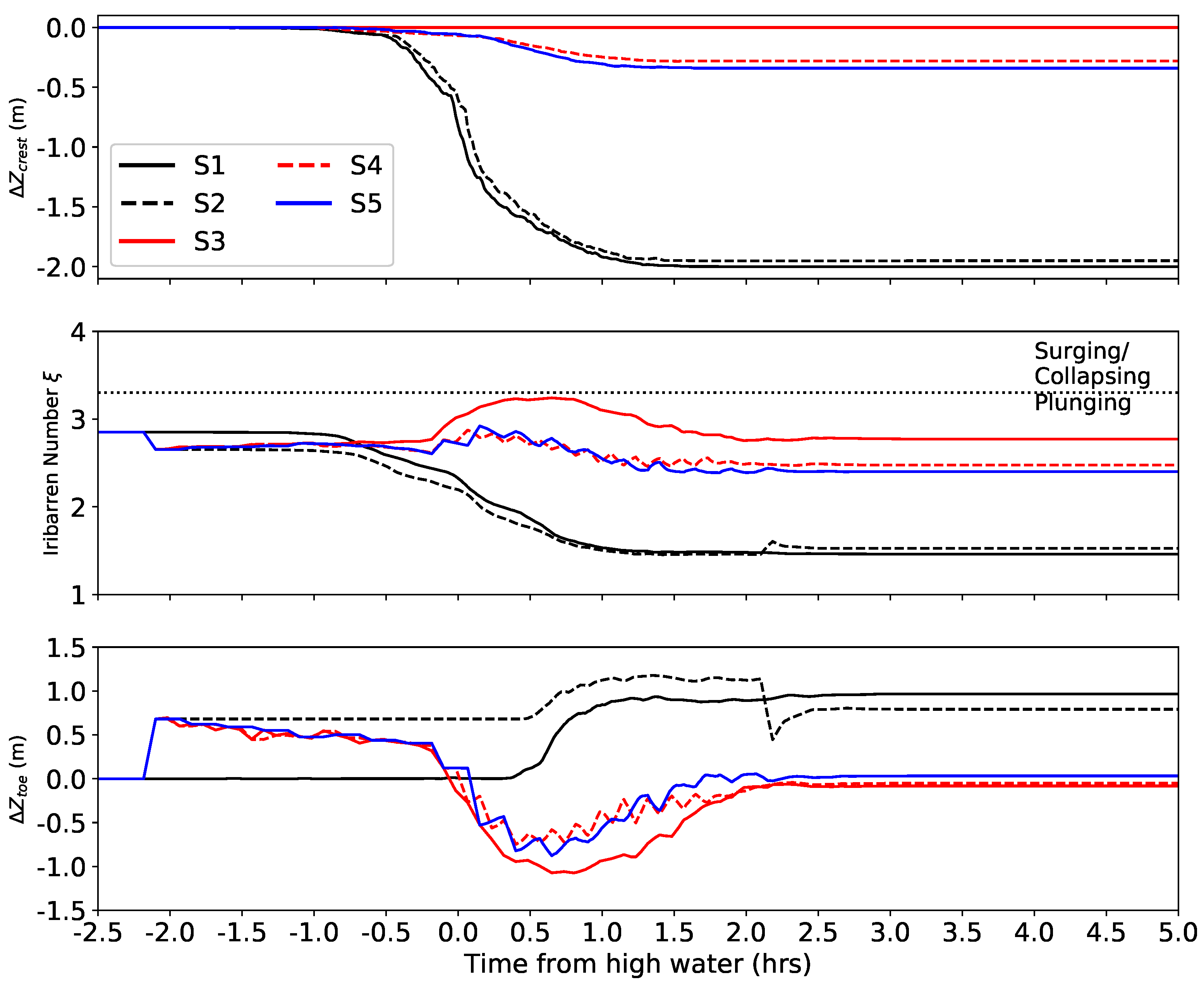
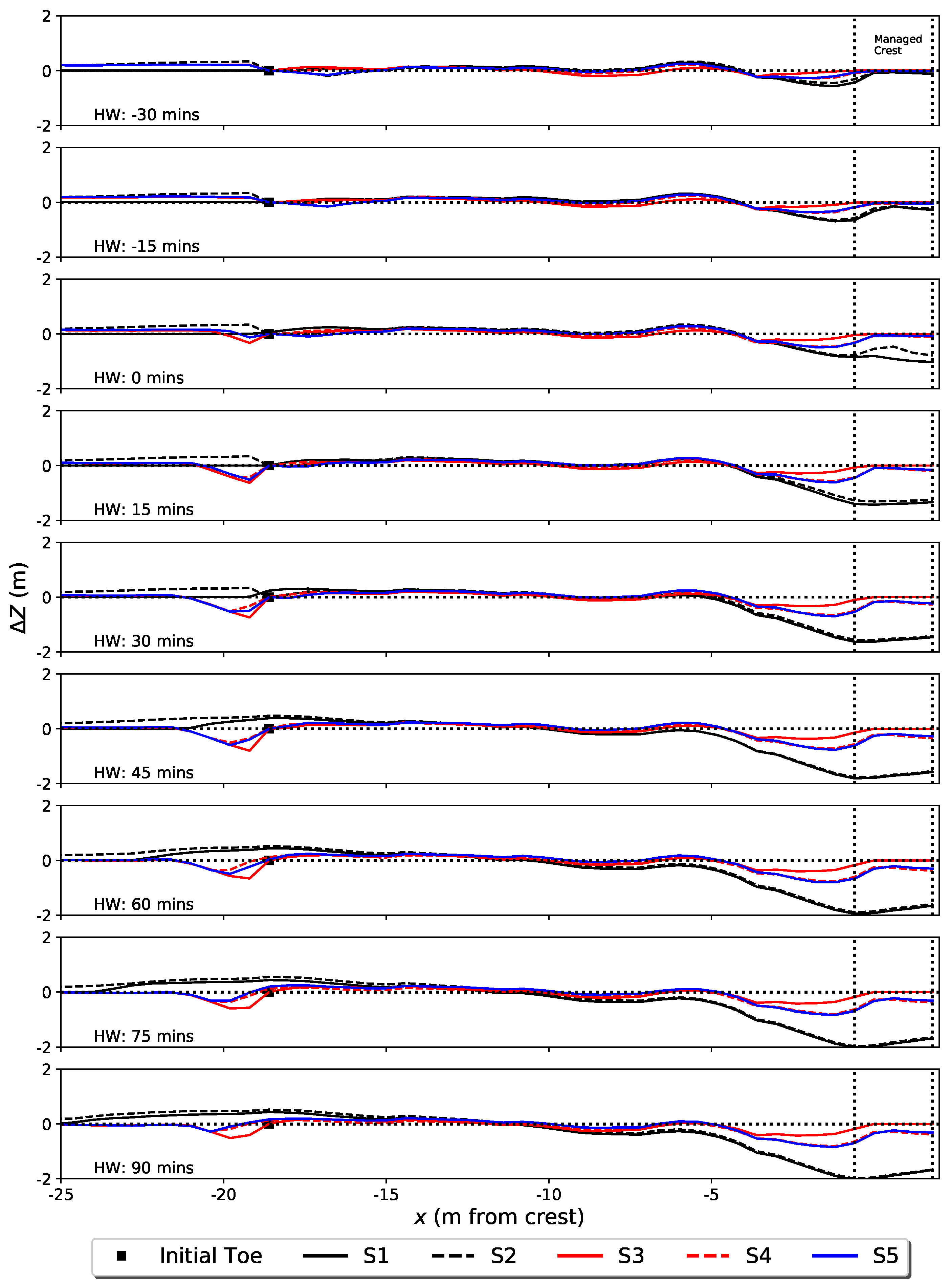
Concentrating on the most extreme wave condition percentiles, Figure 11 demonstrates substantial differences in the morphology of the beach at the barrier toe, the interface of the low-angle sandy terrace and high-angle coarse clastic barrier. The figure confirms that on the flood tide prior to high water there is on-shore transport of sand, leading to sedimentation around the barrier toe. Under S3, while there is some erosion of the area of the barrier crest maintained by the shoreline management policy (Figure 9), there is very little erosion of the barrier at its crest (< ). Results show that for S3–S5, there is a change to net erosion of the barrier toe area at similar times relative to high-water. The three foreshore evolution settings follow a similar trend prior to high water. There is then a switch to net erosion of the barrier toe at high water with the formation of a scour pit. The evolution of the scour pit is shown to vary according to the applied foreshore evolution setting. Figure 11 shows that the scour under S3–S5 begins to commence around high water. Scour under S3 develops further offshore and extends to a greater depth when compared with the other settings. The maximum depth of the scour also occurs closer to the barrier toe when compared to the other foreshore evolution settings. After high water and a switch to net erosion on the foreshore, there is evidence of larger deviation in the trends of erosion between S3–S5. Erosion of the managed section of the barrier at the crest commences at around 30 min prior to high water for S1 and S2. Notably under S3–S5, there is little erosion of the crest itself when compared with S1 and S2. As for morphological change in the upper barrier, there is accretion between x = −7 to −3. Immediately in the lee of this accretion there is a noticeable divergence in . Here, there are three variations in the trend of , with S1 and S2 showing the most substantial erosion (with negligible difference between the two settings), followed by S4 and S5 (with negligible difference between the two settings). Both of these trends show an increasing magnitude of erosion between x = and the barrier crest at x = 0 . The exception is the third trend which is solely S3, where the magnitude of erosion decreases in the same area of the profile.
4.3. Temporal Change in the Iribarren Number under Applied Foreshore Evolution Settings
In Figure 12 we look again at the morphological change through time, but here we consider the changes in the Iribarren number with integrated elevation change across the barrier toe area (). Plunging waves are shown to be the sole breaking wave regime under each of the applied foreshore settings. There are three observed trends in : A substantial decrease in under S1 and S2 occurring at high water, negligible changes under S4 and S5 before and after high water, and an increase under S3, with values almost reaching 3.3, the threshold between plunging and surging/collapsing regimes of wave breaking. The decrease in under S1, S2, S4 and S5 at high water is shown to coincide with increased erosion of the barrier crest. Likewise, at the same time, the increase in under S3 coincides with very little or no erosion of the barrier crest. The peak in is shown to occur at or just after high water under S4 and S5. However, under S3, there is a progressive increase in until around 45 min post-high water.
5. Discussion
The aim of this modeling work was to understand how the characterization of foreshore evolution in XBeach-X (in terms of the frequency at which the sandy, intertidal terrace component of a composite beach is updated) impacts on wave runup and cross-shore sediment transport on a coarse clastic barrier to understand the model’s sensitivity to frequent and infrequent intertidal foreshore updating. Insights into this will provide greater confidence in outputs from storm-impact modeling for similar coastal settings worldwide, and advice for users of the XBeach-X model. Until the capability of storm-impact models such as XBeach-X is developed to specifically resolve the morphodynamics and hydrodynamics of composite gravel beaches in a single model application, this knowledge is critical for informing model setup and overwashing hazard assessments. Attempting to resolve the evolution of a composite beach using solely gravel settings is currently limited by its inability to resolve suspended sediment transport. Likewise using the sandy settings will not resolve the greater permeability and infiltration experienced by gravel barriers.
These scenarios cannot be taken as a prediction of a past or future wave overwashing event. Rather, they demonstrate the impact of and percentile combinations on wave runup and the cross-shore morphologic response of the gravel barrier profile. In this section, the results are discussed in the context of other XBeach modeling studies and we explore the mechanisms behind the model predicting amplified relative wave runup and barrier erosion under less frequent foreshore evolution updates.
5.1. Impact of Foreshore Evolution on Wave Hazard and Erosion
The modeling results demonstrate clear and substantial differences between the less frequent (S1 and S2) and more frequent foreshore updates (S3, S4 and S5) both in terms of wave runup and in cross-shore sediment transport. Under S1, since there is no foreshore evolution updating in this setting and the sand component of the transect is assigned as non-erodible, the only mechanism by which can change is through gravel sediments slumping offshore as the barrier exceeds the angle of repose. On-shore sediment transport of sand on the flood tide occurs regardless of foreshore evolution setting because there is no morphological updating in S2–S5 until the water level exceeds the barrier toe ( m ODN). This explains the rapid increase in identical between the foreshore evolution settings due to the lack of gravel sediment transported offshore due to the water level being lower than the elevation of the barrier. The sedimentation at the barrier toe, rather than the evolution of scour, due to the characterization of the foreshore evolution under S1 and S2 enables a more rapid decrease in and a plunging wave regime persists. This suggests that using a static foreshore in XBeach as per S1, with the only mechanism by which it can morphologically evolve being slumped gravel from the upper barrier is likely to lead to the model over-predicting barrier erosion and wave runup.
Updating foreshore evolution every 5 min (S3) exercises greater wave attenuation in the nearshore, in the lee of the accretion in the profile. This is reflected in both a lower magnitude of erosion in the managed crest, and lower relative wave runup. The extent of erosion in the managed crest of the barrier corresponds to morphological change at the barrier toe. The scour under S4 and S5 remains similar through time, suggesting a foreshore evolution update frequency of <10 min is required to capture the deeper scour at the barrier toe. Halving the update frequency from 10 min to 5 min causes an increase in the maximum scour depth by approximately . The increase in the Iribarren number under S3 around high water to values just under 3.3 is not quite sufficient to trigger a change in the breaking wave regime. Although the increase in stays marginally below the threshold to represent a change in the wave breaking regime, it suggests a transition to more reflective conditions and explains the lower relative wave runup under S3 and fewer hazardous freeboard values. The findings suggest that the method of characterizing foreshore evolution can cause to diverge to both higher and lower values, causing large variability in both the resulting distribution of freeboard values and in the resulting cross-shore sediment transport.
Previous modeling using XBeach-G by McCall et al. [13,23] and the modifications made to the original model by Jamal et al. [24] neglected foreshore evolution in their applications to composite gravel beaches, since their focus was on developing the model for gravel applications. More recent applications of XBeach have attempted to resolve mixed sand–gravel beaches with some element of success [19,20,49], but given the limitations of XBeach discussed above, applications of the model to composite beaches where the evolution of both sand and gravel components are both resolved are currently limited in the literature. This study provides the first application of XBeach where sand and gravel settings are applied to the sandy, intertidal foreshore and coarse clastic barrier components of a composite gravel beach, respectively. The work provides a method for characterizing foreshore evolution within storm-impact modeling of coarse clastic barriers.
5.2. Implications for Modeling Applications on Composite Gravel Beaches
The uncertainty surrounding the feedback between the low-angle sand and high-angle coarse clastic barrier components of a composite gravel beach is shown to lead to major differences in wave runup and cross-shore sediment transport. This variability influences the extent of barrier erosion and back-barrier sediment deposition leading to road closures and hinterland inundation. The results also highlight the potential for the foreshore evolution settings to govern the time of the onset of barrier change, with differences of up to 25 . This may have implications for warning systems, for example road closure times relative to high water. Estimates into the labor and capital required to reform the coarse clastic barrier to its pre-storm profile after an event of a given probability would also be affected by the uncertainty in the control of the foreshore evolution on the response of the barrier. The same implications exist for the development of fragility curves and barrier breaching assessments. This reinforces the need to consider the morphological evolution of both the low-angle and high-angle components of a composite beach. Using S1 and S3 to update foreshore evolution in composite gravel beach applications will provide the user with insights into upper and lower bounds on wave runup and barrier erosion.
5.3. Limitations
There is likely to be some limitations in modeling the time-varying elevation and cross-shore position changes in the barrier toe, since assigning a surface as non-erodible in XBeach-X still allows it to build up through sedimentation; a process unrealistic for on-shore transport of sand onto course-grained highly porous gravel barrier. Although we have tried to mitigate this through setting elevation change above the barrier toe to zero, the limitations of XBeach-X mean that as a consequence, the modeling approach assumes that any on-shore transport of sand does not alter the profile of the gravel barrier. Comparing the model outputs to observational data was not possible, since rigorous validation of the freeboard values would demand high-frequency measurements of the barrier throughout a storm and measurements of overwash hydrodynamics and morphodynamics are often constricted by experimental limitations of fieldwork, particularly when carried out by local authorities rather than for academic research. This paper is constrained by the lack of data against which to validate the results of the storm-impact model. However this limitation does not detract from the importance of exploring the sensitivity of XBeach-X outputs to the foreshore characterization given that sensitivity analysis has been argued to be a useful tool in investigating model behavior [50]. The evolution of the sand and gravel components of a gravel beach cannot be resolved in a single XBeach-X application, and hence the model’s behavior when resolving the sand and gravel components is worthy of investigation. The study does neglect the effect of gradients of alongshore sediment flux given the limitations of the gravel settings in XBeach-X. Although this is shown by Royal Haskoning DHV [26] to be negligible for Newgale given its strongly swash-aligned setting, it would be worthy of investigating in alternate coastal settings, where alongshore sediment transport is of greater relative importance.
6. Conclusions
This study has used XBeach-X to carry out a sensitivity analysis of how characterizing intertidal foreshore evolution within a storm-impact model controls predictions of wave runup and erosion of a composite beach. Previous applications of the model’s gravel settings in the literature focused on mixed sand–gravel beaches, or neglected foreshore evolution within applications to composite beaches. Barrier erosion averaged across all the applied and percentile conditions is an order of magnitude higher when the foreshore remains static or is only updated when the water level reaches the barrier toe on the flood and ebb tides, compared to when the foreshore is updated every 5 or 10 min. The probability density of the most hazardous freeboard values are shown to be a factor of 30 higher when the foreshore is not updated, compared to when the foreshore is updated every 5 min. The simulation where the foreshore was not morphologically updated predicted the highest relative wave runup (), the most substantial barrier erosion and the earliest onset of barrier erosion compared to the other scenarios. The results suggest the greater the frequency at which the foreshore is updated during the gravel barrier modeling, the lower the relative wave runup and the lower the frequency of hazardous freeboard values. Therefore by not updating foreshore evolution throughout the application of a storm-impact model to a gravel barrier is likely to lead to over-prediction of wave runup, by not capturing the scour at the toe of the barrier. The sensitivity analysis highlights the variability in cross-shore sediment transport and wave runup resulting from how foreshore evolution is characterized when modeling a composite gravel beach. Future development of XBeach should concentrate on more explicit representation of the physics which control the feedbacks between the two components of a composite gravel beach, and the ability to spatially vary its sand and gravel settings to different parts of a cross-shore transect, allowing the model to resolve a composite gravel beach in a single model application.
Author Contributions
Conceptualization, B.T.P., J.M.B. and A.J.P.; data collection, B.T.P.; data analysis, B.T.P.; writing—original draft preparation, B.T.P.; writing—review and editing, J.M.B. and A.J.P.; supervision, J.M.B. and A.J.P. All authors have read and agreed to this version of the manuscript.
Funding
Benjamin T. Phillips’s doctoral studentship (to which this article contributes) is funded by Natural Environment Research Council’s Understanding the Earth, Atmosphere and Ocean Doctoral Training Partnership (NE/L002469/1). The studentship is supplemented by West of Wales Coastal Group through a CASE award. This work contributes to the Natural Environment Research Council funded “Physical and biological dynamic coastal processes and their role in coastal recovery (BLUE-coast)” project (NE/N015894/2, NE/N015614/1).
Acknowledgments
The authors would like to thank Emyr Williams (Pembrokeshire County Council and West of Wales Coastal Group) for providing the U.K. Met Office WaveWatchIII data and for discussions regarding the local coastal processes and shoreline management during a field visit to Newgale. The authors would also like to thank the four anonymous reviewers for their constructive comments which have enriched the manuscript.
Conflicts of Interest
The authors declare no conflict of interest. The funders had no role in the design of the study; in the collection, analyses, or interpretation of data; in the writing of the manuscript, or in the decision to publish the results.
References
- Masselink, G.; Scott, T.; Poate, T.; Russell, P.; Davidson, M.; Conley, D. The extreme 2013/2014 winter storms: Hydrodynamic forcing and coastal response along the southwest coast of England. Earth Surf. Process. Landf. 2016, 41, 378–391. [Google Scholar] [CrossRef] [Green Version]
- Tamarin, T.; Kaspi, Y. The poleward shift of storm tracks under global warming: A Lagrangian perspective. Geophys. Res. Lett. 2017, 44, 10666–10674. [Google Scholar] [CrossRef]
- Vitousek, S.; Barnard, P.L.; Fletcher, C.H.; Frazer, N.; Storlazzi, C.D. Doubling of coastal flooding frequency within decades due to sea-level rise. Sci. Rep. 2017, 7, 1399. [Google Scholar] [CrossRef]
- Moses, C.A.; Williams, R.B.G. Artificial beach recharge: The South East England experience. Z. Fur Geomorphol. Suppl. Issues 2008, 52, 107–124. [Google Scholar] [CrossRef]
- McCall, R.; de Vries, J.V.T.; Plant, N.; Dongeren, A.V.; Roelvink, J.; Thompson, D.; Reniers, A. Two-dimensional time dependent hurricane overwash and erosion modeling at Santa Rosa Island. Coast. Eng. 2010, 57, 668–683. [Google Scholar] [CrossRef]
- Lorenzo-Trueba, J.; Ashton, A.D. Rollover, drowning, and discontinuous retreat: Distinct modes of barrier response to sea-level rise arising from a simple morphodynamic model. J. Geophys. Res. Earth Surf. 2014, 119, 779–801. [Google Scholar] [CrossRef] [Green Version]
- Mellett, C.L.; Plater, A.J. Drowned Barriers as Archives of Coastal-Response to Sea-Level Rise. In Barrier Dynamics and Response to Changing Climate; Moore, L.J., Murray, A.B., Eds.; Springer International Publishing: Cham, Switzerland, 2018; pp. 57–89. [Google Scholar] [CrossRef]
- Jennings, R.; Shulmeister, J. A field based classification scheme for gravel beaches. Mar. Geol. 2002, 186, 211–228. [Google Scholar] [CrossRef]
- Roelvink, D.; Reniers, A.; van Dongeren, A.; van Thiel de Vries, J.; McCall, R.; Lescinski, J. Modelling storm impacts on beaches, dunes and barrier islands. Coast. Eng. 2009, 56, 1133–1152. [Google Scholar] [CrossRef]
- Grases, A.; Gracia, V.; García-León, M.; Lin-Ye, J.; Sierra, J.P. Coastal Flooding and Erosion under a Changing Climate: Implications at a Low-Lying Coast (Ebro Delta). Water 2020, 12, 346. [Google Scholar] [CrossRef] [Green Version]
- Phillips, B.T.; Brown, J.M.; Bidlot, J.R.; Plater, A.J. Role of beach morphology in wave overtopping hazard assessment. J. Mar. Sci. Eng. 2017, 5, 1. [Google Scholar] [CrossRef] [Green Version]
- Dissanayake, P.; Brown, J.; Wisse, P.; Karunarathna, H. Effects of storm clustering on beach/dune evolution. Mar. Geol. 2015, 370, 63–75. [Google Scholar] [CrossRef]
- McCall, R.; Masselink, G.; Poate, T.; Roelvink, J.; Almeida, L. Modelling the morphodynamics of gravel beaches during storms with XBeach-G. Coast. Eng. 2015, 103, 52–66. [Google Scholar] [CrossRef]
- Poate, T.G.; McCall, R.T.; Masselink, G. A new parameterisation for runup on gravel beaches. Coast. Eng. 2016, 117, 176–190. [Google Scholar] [CrossRef] [Green Version]
- Stockdon, H.; Holman, R.; Howd, P.; Sallenger, A.H., Jr. Empirical parameterization of setup, swash, and runup. Coast. Eng. 2006, 53, 573–588. [Google Scholar] [CrossRef]
- Sallenger, A.H., Jr. Storm impact scale for barrier islands. J. Coast. Res. 2000, 16, 890–895. [Google Scholar]
- Plomaritis, T.A.; Ferreira, Ã.; Costas, S. Regional assessment of storm related overwash and breaching hazards on coastal barriers. Coast. Eng. 2018, 1, 124–133. [Google Scholar] [CrossRef]
- Donnelly, C.; Larson, M.; Hanson, H. A numerical model of coastal overwash. Proc. Inst. Civ. Eng.-Marit. Eng. 2009, 162, 105–114. [Google Scholar] [CrossRef] [Green Version]
- Brown, S.I.; Dickson, M.E.; Kench, P.S.; Bergillos, R.J. Modelling gravel barrier response to storms and sudden relative sea-level change using XBeach-G. Mar. Geol. 2019, 4, 164–175. [Google Scholar] [CrossRef]
- Bergillos, R.J.; Masselink, G.; Ortega-Sánchez, M. Coupling cross-shore and longshore sediment transport to model storm response along a mixed sand-gravel coast under varying wave directions. Coast. Eng. 2017, 129, 93–104. [Google Scholar] [CrossRef] [Green Version]
- Bergillos, R.J.; Rodríguez-Delgado, C.; Ortega-Sánchez, M. Advances in management tools for modeling artificial nourishments in mixed beaches. J. Mar. Syst. 2017, 1, 1–13. [Google Scholar] [CrossRef]
- Pollard, J.; Spencer, T.; Brooks, S.; Christie, E.; Möller, I. Understanding spatio-temporal barrier dynamics through the use of multiple shoreline proxies. Geomorphology 2020, 3, 107058. [Google Scholar] [CrossRef]
- McCall, R.T.; Masselink, G.; Poate, T.G.; Roelvink, J.A.; Almeida, L.P.; Davidson, M.; Russell, P.E. Modelling storm hydrodynamics on gravel beaches with XBeach-G. Coast. Eng. 2014, 91, 231–250. [Google Scholar] [CrossRef] [Green Version]
- Jamal, M.; Simmonds, D.; Magar, V. Modelling gravel beach dynamics with XBeach. Coast. Eng. 2014, 89, 20–29. [Google Scholar] [CrossRef]
- Masselink, G.; McCall, R.; Poate, T.; van Geer, P. Modelling storm response on gravel beaches using XBeach-G. Proc. ICE Marit. Eng. 2014, 167, 173–191. [Google Scholar] [CrossRef] [Green Version]
- Royal Haskoning DHV. Newgale Shingle Bank Vulnerability Assessment; Technical Report; Haskoning DHV Ltd.: Peterborough, UK, 2014. [Google Scholar]
- ESRI. World Imagery; ESRI: Redlands, CA, USA, 2020. [Google Scholar]
- Natural Resources Wales. Shoreline Management Plan (SMP) 2; Natural Resources Wales: Cardiff, UK, 2019. [Google Scholar]
- Telegraph. Newgale Beach, Pembrokeshire. Telegraph. 2019. Available online: https://www.telegraph.co.uk/travel/galleries/britains-best-shingle-beaches/newgale-beach-pembrokeshire/ (accessed on 10 November 2020).
- Western Telegraph. Managed Retreat from Newgale ‘in Next 60 Years’. Western Telegraph. 2014. Available online: https://www.westerntelegraph.co.uk/news/11083509.managed-retreat-from-newgale-in-next-60-years/ (accessed on 10 November 2020).
- Prime, T.; Brown, J.M.; Plater, A.J. Flood inundation uncertainty: The case of a 0.5% annual probability flood event. Environ. Sci. Policy 2016, 59, 1–9. [Google Scholar] [CrossRef] [Green Version]
- Bendoni, M.; Georgiou, I.; Roelvink, D.; Oumeraci, H. Numerical modelling of the erosion of marsh boundaries due to wave impact. Coast. Eng. 2019, 152, 103514. [Google Scholar] [CrossRef]
- Garzon, J.L.; Miesse, T.; Ferreira, C.M. Field-based numerical model investigation of wave propagation across marshes in the Chesapeake Bay under storm conditions. Coast. Eng. 2019, 146, 32–46. [Google Scholar] [CrossRef]
- Splinter, K.D.; Carley, J.T.; Golshani, A.; Tomlinson, R. A relationship to describe the cumulative impact of storm clusters on beach erosion. Coast. Eng. 2014, 83, 49–55. [Google Scholar] [CrossRef]
- Dongeren, A.V.; Lowe, R.; Pomeroy, A.; Minh, D.; Roelvink, D.; Symonds, G.; Ranasinghe, R. Numerical modeling of low-frequency wave dynamics over a fringing coral reef. Coast. Eng. 2013, 73, 178–190. [Google Scholar] [CrossRef]
- Quataert, E.; Storlazzi, C.; Rooijen, A.; Cheriton, O.; Dongeren, A. The influence of coral reefs and climate change on wave-driven flooding of tropical coastlines. Geophys. Res. Lett. 2015, 6407–6415. [Google Scholar] [CrossRef]
- Williams, J.J.; de Alegría-Arzaburu, A.R.; McCall, R.T.; Van Dongeren, A. Modelling gravel barrier profile response to combined waves and tides using XBeach: Laboratory and field results. Coast. Eng. 2012, 63, 62–80. [Google Scholar] [CrossRef]
- Van Rijn, L.C. A simple general expression for longshore transport of sand, gravel and shingle. Coast. Eng. 2014, 90, 23–39. [Google Scholar] [CrossRef]
- Lyddon, C.; Brown, J.M.; Leonardi, N.; Plater, A.J. Flood Hazard Assessment for a Hyper-Tidal Estuary as a Function of Tide-Surge-Morphology Interaction. Estuaries Coasts 2018, 41, 1565–1586. [Google Scholar] [CrossRef] [Green Version]
- CEFAS. WaveHindcast. (Note: The WaveWatchIII data is Provided by the U.K. Met Office and Hosted by the Centre for Environment, Fisheries and Aquaculture Science (CEFAS) on a Platform Funded by the Environment Agency.). Available online: http://wavenet.cefas.co.uk/hindcast (accessed on 29 September 2010).
- Hasselmann, K.; Barnett, T.; Bouws, E.; Carlson, H.; Cartwright, D.; Enke, K.; Ewing, J.; Gienapp, H.; Hasselmann, D.; Kruseman, P.; et al. Measurements of wind-wave growth and swell decay during the Joint North Sea Wave Project (JONSWAP). Dtsch. Hydrogr. Inst. 1973, 8, 1–95. [Google Scholar]
- National Oceanography Centre. POLTIPS-3 Coastal Tidal Software; National Oceanography Centre: Liverpool, UK, 2016. [Google Scholar]
- National Tidal and Sea Level Facility. Highest & Lowest Predicted Tides at Milford Haven; National Tidal and Sea Level Facility: Liverpool, UK, 2019. [Google Scholar]
- Natural Resources Wales. LiDAR Dataset Wales. Available online: https://libcat.naturalresources.wales/webview/?tiarray=full&oid=116814 (accessed on 14 August 2020).
- Hallermeier, R.J. A profile zonation for seasonal sand beaches from wave climate. Coast. Eng. 1981, 4, 253–277. [Google Scholar] [CrossRef]
- OceanWise. 1 Arcsecond Bathymetry—Marine Themes Digital Elevation Model (DEM). Available online: https://digimap.edina.ac.uk/webhelp/marine/data_information/products_available/1_arcsecond_bathymetry.htm (accessed on 15 September 2020).
- Deltares. XBeach Toolbox. Available online: https://repos.deltares.nl/repos/OpenEarthTools/trunk/matlab/applications/xbeach/ (accessed on 22 October 2020).
- Battjes, J. Surf Similarity. In Proceedings of the 14th International Conference on Coastal Engineering 1974, Copenhagen, Denmark, 24–28 June 1974; pp. 466–480. [Google Scholar] [CrossRef]
- Dornbusch, U. Design requirement for mixed sand and gravel beach defences under scenarios of sea level rise. Coast. Eng. 2017, 124, 12–24. [Google Scholar] [CrossRef]
- Pianosi, F.; Beven, K.; Freer, J.; Hall, J.W.; Rougier, J.; Stephenson, D.B.; Wagener, T. Sensitivity analysis of environmental models: A systematic review with practical workflow. Environ. Model. Softw. 2016, 79, 214–232. [Google Scholar] [CrossRef]
Figure 1.
(A) Aerial view of Newgale, its location within the U.K. and the SMP2 policy units for the village [27,28], (B) the gravel barrier and intertidal sandy foreshore at Newgale looking towards the south-west [29] and (C) the aftermath of the January 2014 storm [30]. The Duke of Edinburgh Inn is shown on (A,C) to assist orientation.
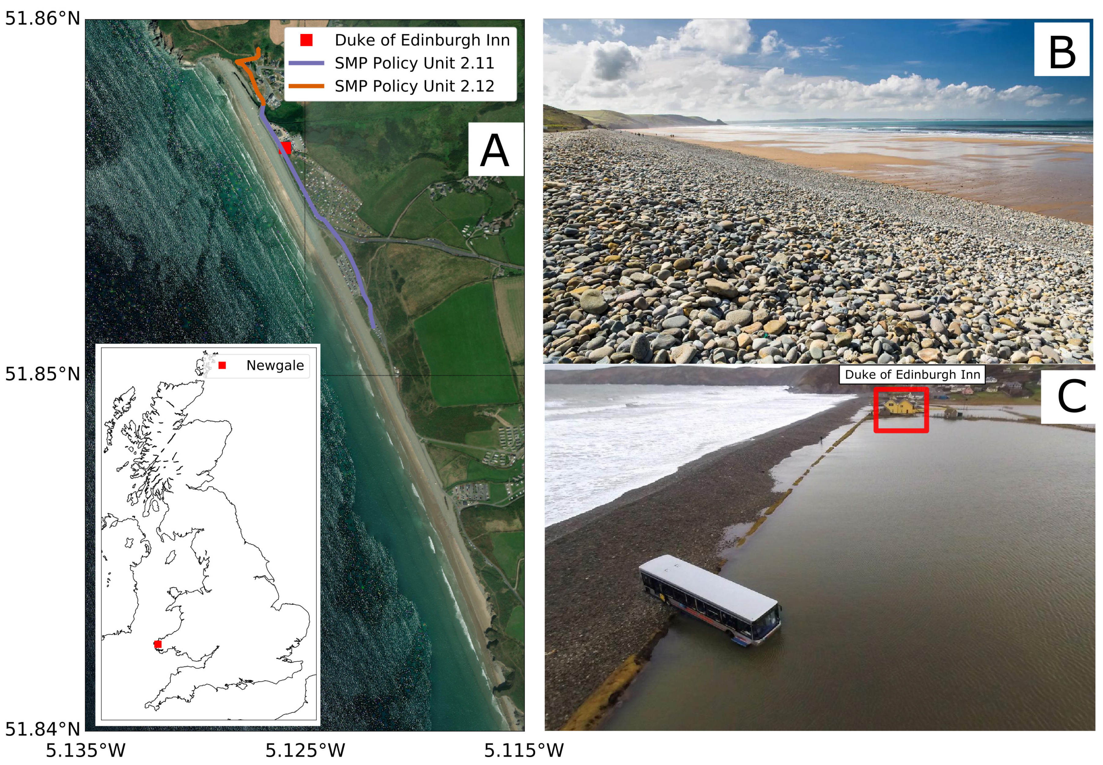
Figure 2.
Location of the cross-shore profile, WaveWatchIII node and Milford Haven tide gauge, and the location of Newgale within the U.K.
Figure 2.
Location of the cross-shore profile, WaveWatchIII node and Milford Haven tide gauge, and the location of Newgale within the U.K.
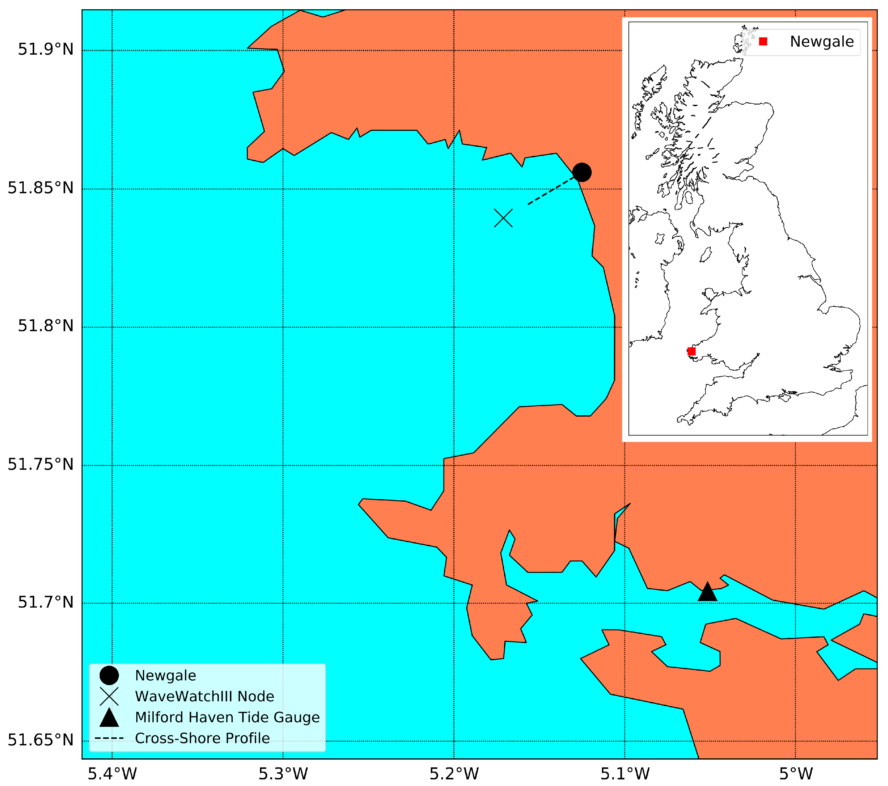
Figure 3.
and values at each high water (Table 2), and the corresponding wave direction. High-water times are obtained from the Milford Haven tide gauge. , and wave direction data is obtained from the U.K. Met Office WaveWatchIII model [40].

Figure 4.
The applied highest astronomical tidal curve, calculated by the POLTIPS3 tidal prediction software.
Figure 4.
The applied highest astronomical tidal curve, calculated by the POLTIPS3 tidal prediction software.

Figure 5.
Applied cross-shore profile used in XBeach-X with the intertidal sandy foreshore and gravel barrier components of the composite gravel beach. The upper panel provides additional detail in the nearshore, and the dashed line at 7 m ODN represents the elevation above which the barrier width is artifically maintained.
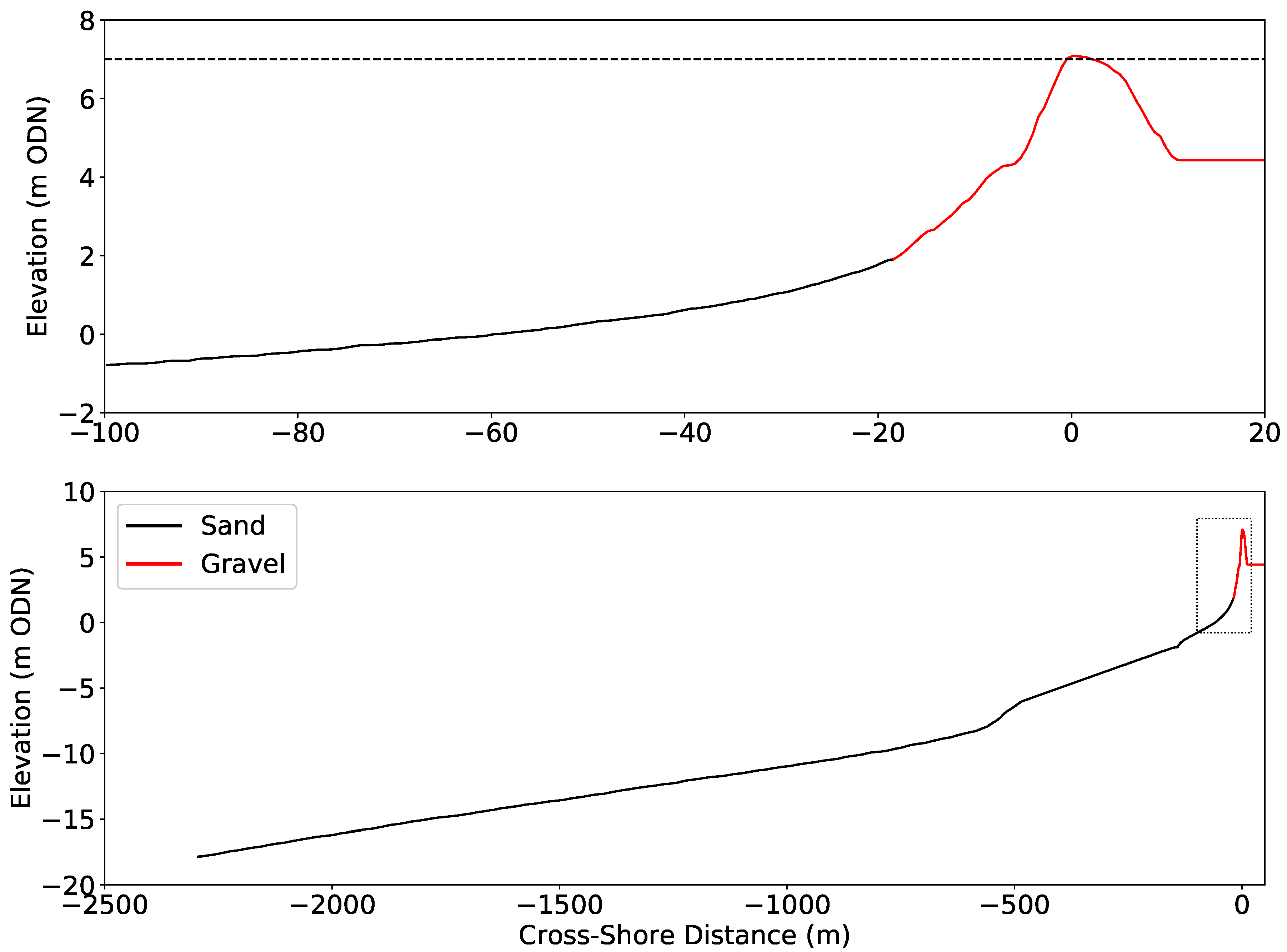
Figure 6.
A schematic of proxies used to describe the results of the XBeach-X modeling.
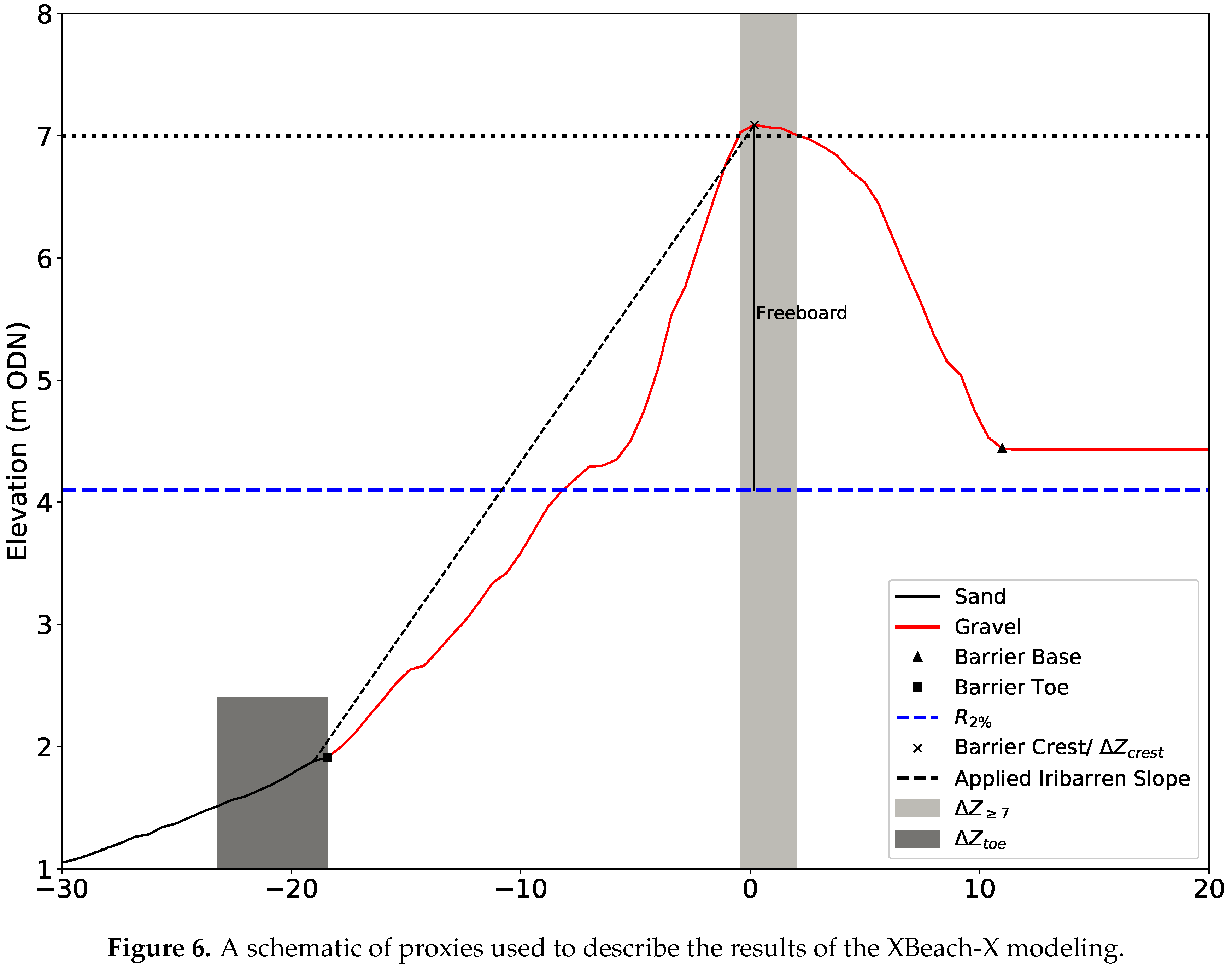
Figure 7.
Distribution of modeled freeboard values under each - percentile combination and HAT for S1–S5. The distribution consists of freeboard values calculated when the water level exceeds the barrier toe (≥ m ODN).
Figure 7.
Distribution of modeled freeboard values under each - percentile combination and HAT for S1–S5. The distribution consists of freeboard values calculated when the water level exceeds the barrier toe (≥ m ODN).
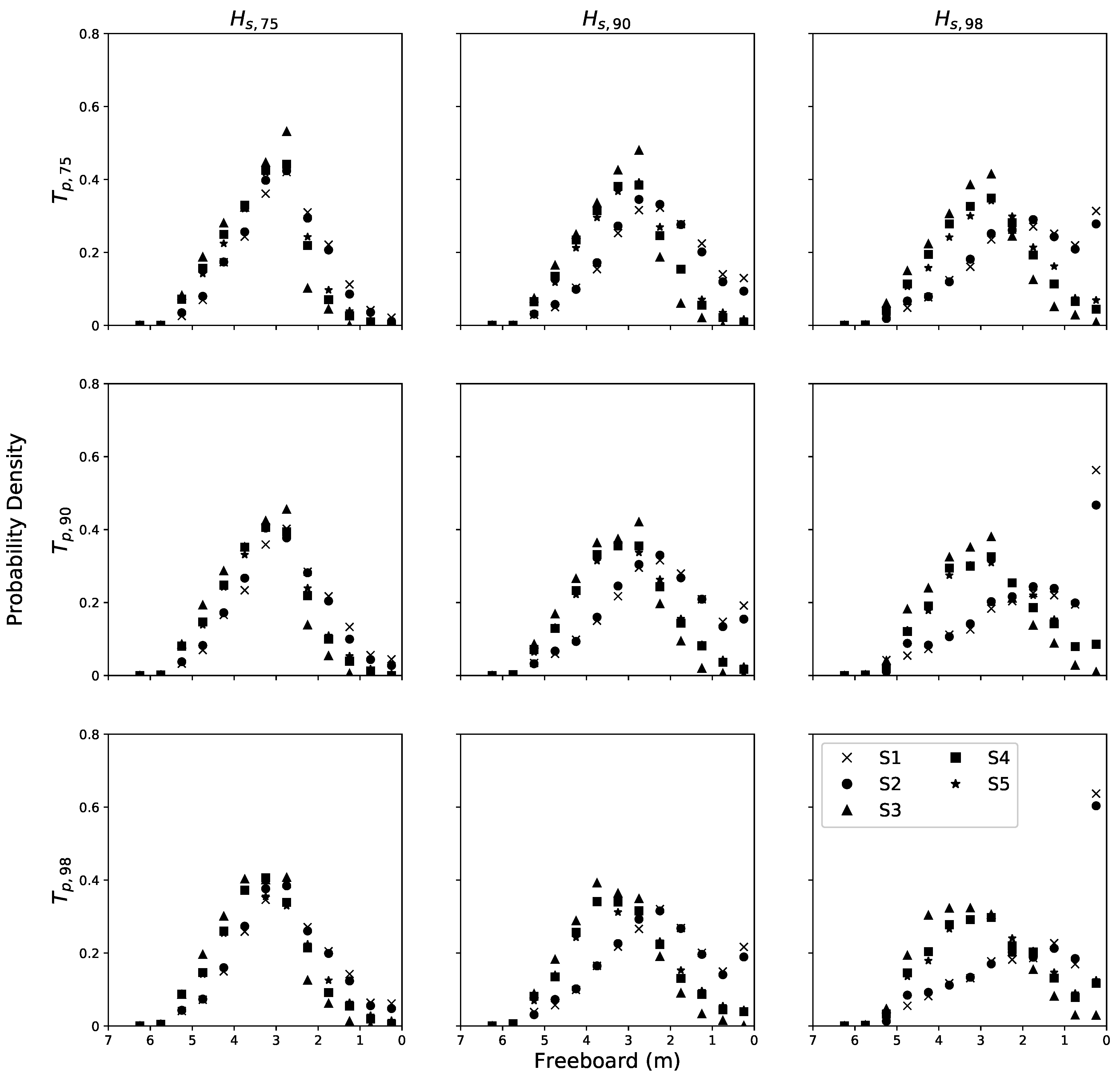
Figure 8.
Time-averaged (one-minute) relative wave runup averaged across all 25 wave percentile combinations for S1 to S5.
Figure 8.
Time-averaged (one-minute) relative wave runup averaged across all 25 wave percentile combinations for S1 to S5.

Figure 9.
Cumulative integrated elevation change of the barrier crest (above 7 m ODN) using S1 to S5 for each and combination under the highest astronomical tide.
Figure 9.
Cumulative integrated elevation change of the barrier crest (above 7 m ODN) using S1 to S5 for each and combination under the highest astronomical tide.
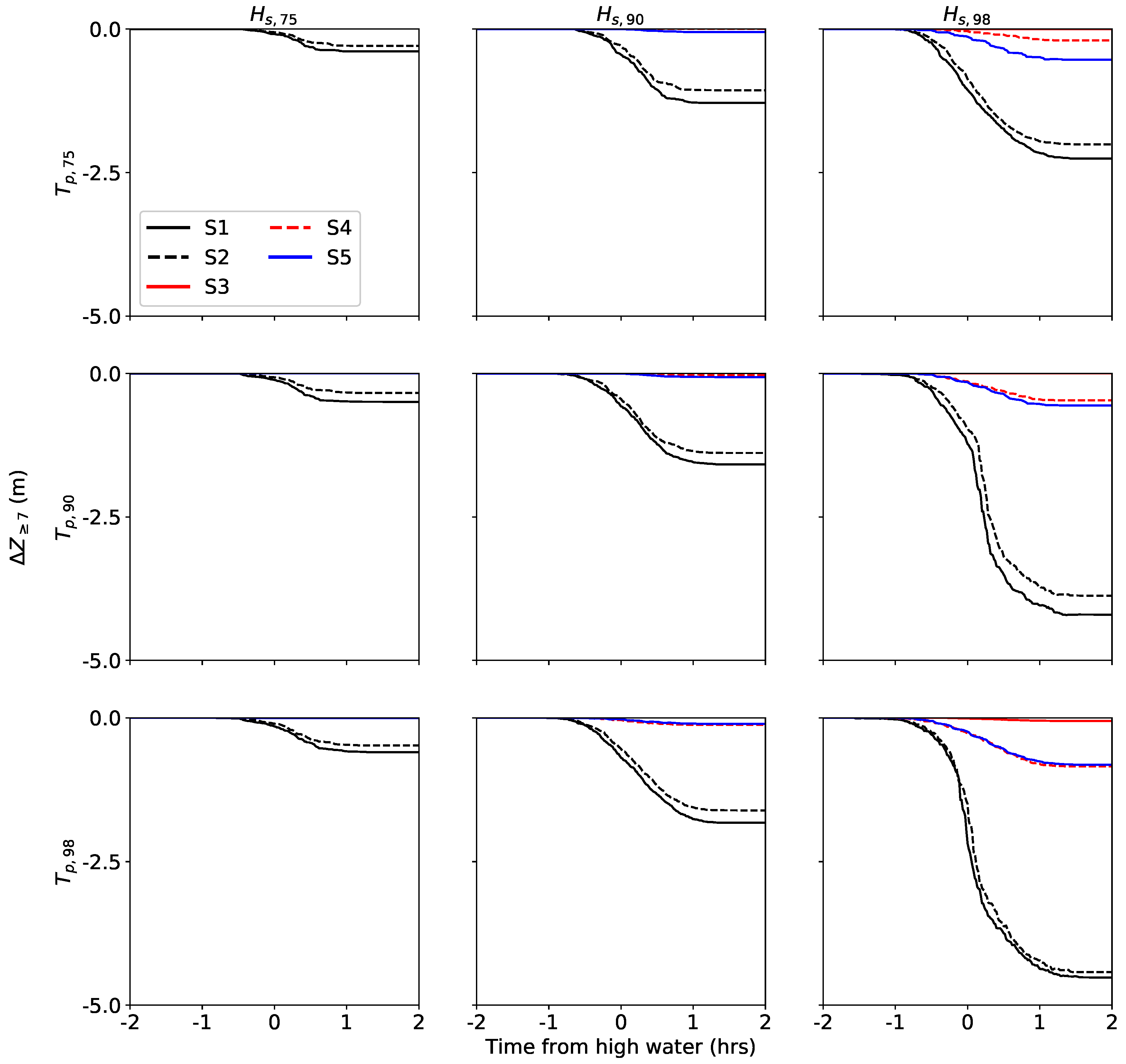
Figure 10.
Cumulative integrated elevation change of the area from the base of the back barrier to the model’s landward boundary, using S1 to S5 for each and combination under the highest astronomical tide.
Figure 10.
Cumulative integrated elevation change of the area from the base of the back barrier to the model’s landward boundary, using S1 to S5 for each and combination under the highest astronomical tide.
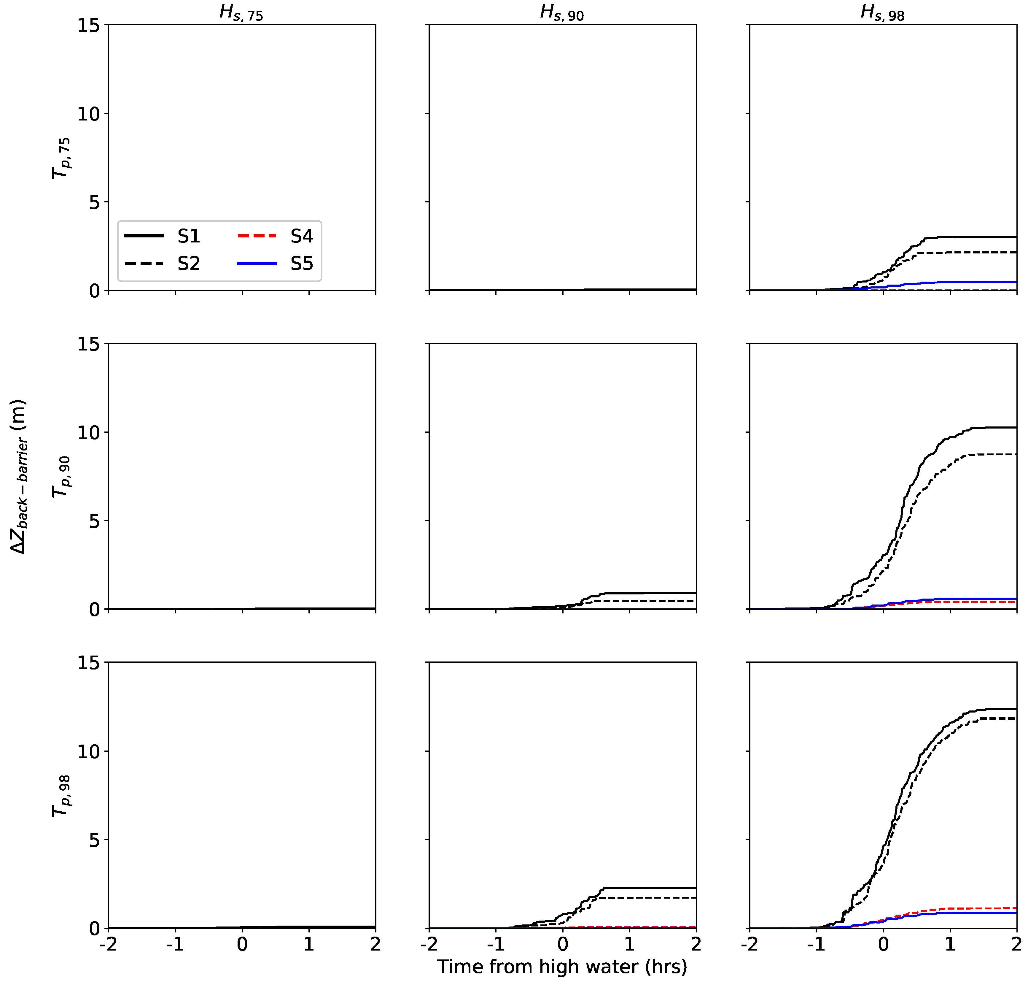
Figure 11.
Nearshore elevation change () across two hours either side of high water under S1–S5. Positive values represent accretion, and negative values represent erosion. The most extreme wave percentile combination is applied, and under highest astronomical tide. The dotted vertical lines denote the area of the crest that exceeds 7 m ODN, the height above which is artificially maintained to ensure sufficient width. The dotted horizontal line is 0 . The black square denotes the barrier toe at the start of the model run.

Figure 12.
Changes in elevation of the barrier crest (), the Iribarren number (, 5 min moving average) and changes in integrated elevation change in the barrier toe area (, 5 min moving average) through time, under each of the applied foreshore evolution settings. The most extreme wave percentile combination is applied, and under highest astronomical tide. The dotted horizontal line at = 3.3 denotes the threshold between plunging and surging/collapsing breaking wave regimes.

Table 1.
SMP2 managed realignment (MR) and no active intervention (NAI) policies for each policy unit in Newgale shown on Figure 1.
Table 1.
SMP2 managed realignment (MR) and no active intervention (NAI) policies for each policy unit in Newgale shown on Figure 1.
| Policy Unit | 0–20 Years | 20–50 Years | 50–100 Years | Intention |
|---|---|---|---|---|
| 2.11 | MR | MR | NAI | Manage shingle on the road with the long-term intent of allowing the gravel barrier to behave naturally |
| 2.12 | MR | MR | MR | Manage the cliffs and stream position to sustain the upper village |
Table 2.
The 10th, 50th, 75th, 90th and 98th percentiles of and in Figure 3, obtained from the U.K. Met Office WaveWatchIII model. The first occurrence of each value is accompanied by the percentage of the time the percentile is exceeded based on the 36 years of WaveWatchIII data, in parentheses.
Table 2.
The 10th, 50th, 75th, 90th and 98th percentiles of and in Figure 3, obtained from the U.K. Met Office WaveWatchIII model. The first occurrence of each value is accompanied by the percentage of the time the percentile is exceeded based on the 36 years of WaveWatchIII data, in parentheses.
| Scenario | () | () |
|---|---|---|
| 1 | 0.36 () | 5.52 () |
| 2 | 0.94 () | 5.52 |
| 3 | 1.50 () | 5.52 |
| 4 | 2.18 () | 5.52 |
| 5 | 3.56 () | 5.52 |
| 6 | 0.36 | 9.52 () |
| 7 | 0.94 | 9.52 |
| 8 | 1.50 | 9.52 |
| 9 | 2.18 | 9.52 |
| 10 | 3.56 | 9.52 |
| 11 | 0.36 | 11.49 () |
| 12 | 0.94 | 11.49 |
| 13 | 1.50 | 11.49 |
| 14 | 2.18 | 11.49 |
| 15 | 3.56 | 11.49 |
| 16 | 0.36 | 13.33 () |
| 17 | 0.94 | 13.33 |
| 18 | 1.50 | 13.33 |
| 19 | 2.18 | 13.33 |
| 20 | 3.56 | 13.33 |
| 21 | 0.36 | 15.15 () |
| 22 | 0.94 | 15.15 |
| 23 | 1.50 | 15.15 |
| 24 | 2.18 | 15.15 |
| 25 | 3.56 | 15.15 |
Table 3.
The five applied foreshore evolution scenarios in the XBeach-X gravel simulations.
| Scenario | Description |
|---|---|
| S1 | There is no updating of the foreshore evolution. The initial, sandy foreshore shown in Figure 5 remains static throughout the simulation. |
| S2 | The foreshore is updated twice according to the evolved profile at the equivalent point in time from the XBeach-X outputs with the sandy settings enabled and the gravel barrier assigned as non-erodible. The first update occurs when the water level exceeds the barrier toe ( m ODN) on the flood tide. The second and final update occurs when the water level recedes below the barrier toe on the ebb tide. |
| S3 | As S2, but additional foreshore updates occur every 5 min while the water level exceeds the barrier toe. |
| S4 | As S2, but additional foreshore updates occur every 10 min while the water level exceeds the barrier toe. |
| S5 | As S2, but additional foreshore updates occur every 15 min while the water level exceeds the barrier toe. |
Table 4.
Integrated elevation change for the barrier crest and back barrier averaged across each and percentile combination for each of the applied foreshore evolution settings.
Table 4.
Integrated elevation change for the barrier crest and back barrier averaged across each and percentile combination for each of the applied foreshore evolution settings.
| Foreshore Evolution Setting | Mean Barrier Erosion (m) | Mean Land Sedimentation (m) |
|---|---|---|
| S1 | −0.79 | 1.17 |
| S2 | −0.71 | 1.00 |
| S3 | 0.00 | 0.00 |
| S4 | −0.07 | 0.06 |
| S5 | −0.11 | 0.08 |
Publisher’s Note: MDPI stays neutral with regard to jurisdictional claims in published maps and institutional affiliations. |
© 2020 by the authors. Licensee MDPI, Basel, Switzerland. This article is an open access article distributed under the terms and conditions of the Creative Commons Attribution (CC BY) license (http://creativecommons.org/licenses/by/4.0/).
Share and Cite
MDPI and ACS Style
Phillips, B.T.; Brown, J.M.; Plater, A.J. Modeling Impact of Intertidal Foreshore Evolution on Gravel Barrier Erosion and Wave Runup with XBeach-X. J. Mar. Sci. Eng. 2020, 8, 914. https://doi.org/10.3390/jmse8110914
AMA Style
Phillips BT, Brown JM, Plater AJ. Modeling Impact of Intertidal Foreshore Evolution on Gravel Barrier Erosion and Wave Runup with XBeach-X. Journal of Marine Science and Engineering. 2020; 8(11):914. https://doi.org/10.3390/jmse8110914
Chicago/Turabian StylePhillips, Benjamin T., Jennifer M. Brown, and Andrew J. Plater. 2020. "Modeling Impact of Intertidal Foreshore Evolution on Gravel Barrier Erosion and Wave Runup with XBeach-X" Journal of Marine Science and Engineering 8, no. 11: 914. https://doi.org/10.3390/jmse8110914
Note that from the first issue of 2016, this journal uses article numbers instead of page numbers. See further details here.