Applicability of the Goda–Takahashi Wave Load Formula for Vertical Slender Hydraulic Structures

Abstract

Vertical slender hydraulic structures such as sluices, navigation locks, or storm-surge barriers are often dynamically loaded by waves. For a safe and economic design, an accurate description of the wave loads is needed. A widely used formula for this purpose is the Goda–Takahashi wave load formula (GT). It was derived for the assessment of gravity-based caisson breakwaters. Due to its many advantages, the formula is also often employed for the assessment of vertical slender hydraulic structures, although its applicability to those type of structures was never fully demonstrated. This study provides insights in the applicability of GT for vertical slender hydraulic structures. This is done based on a literature review on the historical backgrounds of GT, and an investigation of several case-studies. In the case-studies, the equivalent-static wave loads for caisson breakwaters in scope of GT are compared with those for vertical slender hydraulic structures. The results show that GT can safely be applied for vertical slender hydraulic structures loaded by pulsating wave loads, but that systematic over- or under-estimations are expected for breaking or impact wave loads. For individual cases, differences up to 200% were obtained. These large over- or under-estimations underline the need for an improvement of the current design tools for vertical slender hydraulic structures loaded by breaking or impact wave loads.

1. Introduction

Vertical slender hydraulic structures such as sluices, navigation locks, storm-surge barriers, or splash barriers are often loaded by waves. Especially when subjected to breaking or impact waves, these wave loads can be large, governing the design of the structure.

Under certain conditions, the (time-varying) wave loads may cause a dynamic response of the structure, either increasing or decreasing the cross-sectional forces as compared to the static application of the wave loads. For a proper determination of these cross-sectional forces a dynamic assessment needs to be conducted, taking into account the time-histories of the wave load and the dynamic characteristics of the structure, see e.g., [1,2]. A dynamic assessment can however be complex and time-consuming, and requires information that is often not directly available to the engineer (e.g., the time-histories of the design wave load). In those situations, the engineer is deemed to use more simplistic and practical design methods, which predict equivalent-static wave loads on the basis of a limited number of design parameters, and which account for the dynamic behavior of the structure implicitly.

A popular engineering formula for this purpose regards the Goda–Takahashi wave load formula (GT) [3], see Section 2.5. It predicts equivalent-static wave loads for the sliding and overturning failure mechanism of caisson breakwaters, on the basis of incoming wave characteristics (height, period), structure geometry, and foreshore bathymetry. The formula accounts implicitly for the dynamic response to the whole range of pulsating, (post) breaking, and impact wave loads.

Due to its simplicity, and due to the lack of designated engineering models for vertical slender hydraulic structures, the Goda–Takahashi wave load formula (GT) is also recommended in several codes and standards for the assessment of vertical slender hydraulic structures, see e.g., [4,5,6,7]. However, essential differences exist between the dynamic behavior of caisson breakwaters and vertical slender hydraulic structures. Caisson breakwaters are heavy, monolithic structures of which the design is determined by global failure mechanisms such as sliding and overturning. Vertical slender hydraulic structures are typically lightweight and composed of a number of components (beams, plates, etc.) that are each assessed individually and on the cross-sectional level.

To account for these differences, some references point out the inadequacy of GT for certain design situations. E.g., in the Dutch Design Guidelines for Slender Hydraulic Structures [6] the application of GT is discouraged in case of ‘lightweight water retaining elements’ and ‘significant wave heights higher than half the water depth combined steep sea bottoms above 1:50’. Allsop et al. [8] discourage the application of GT in case of ‘wave loads of short duration and with limited spatial extent’.

Although these disclaimers provide a good first indication on the applicability of GT to vertical slender hydraulic structures, they are often based on expert knowledge without much further substantiation. This lack of substantiation sometimes leads to ambiguity for the practicing engineer; e.g., which elements should be considered as ‘lightweight’, or what is exactly defined as a wave load with ‘short duration’ or ’limited spatial extent’? As importantly, what is the potential error we make when we apply GT nonetheless?

The aim of this study is therefore to gain a better insight in the valid application area of GT for vertical slender hydraulic structures, and to provide a first estimate on the potential error one makes when GT is applied outside of this valid application area.

The study focuses on vertical slender hydraulic structures, which are loaded by depth-induced breaking wave loads only; wave loads caused by other sources (e.g., wave impacts due to the presence of confinements [9,10]) or aspects related to wave absorption (e.g., due to perforated plates [11]) are not considered here.

This study is conducted as follows. First, a literature review is performed on the definition of equivalent-static wave loads, the (differences in) dynamic behavior of caisson breakwaters and slender hydraulic structures, and the historical backgrounds of the GT wave load formula (Section 2). Then, a number of case-studies is selected for which the potential over- or under-estimation is quantified when GT is applied to slender hydraulic structures (Section 3 and Section 4). Based on the results, it is investigated how the obtained over- or under-estimations relate to other sources of uncertainties inherent to GT, and practical recommendations for the (current and future) assessment of slender hydraulic structures are given (Section 5). The conclusions of this study are presented in Section 6.

2. Literature Review

2.1. Equivalent-Static Wave Loads

This paper investigates the extent to which GT can be applied to predict equivalent-static wave loads for vertical slender hydraulic structures. For this a clear definition of equivalent-static wave loads is needed. Consider an incoming wave load $P\left(t\right)$ with maximum value $P_{\max }$ exerted upon the structure. Depending on the dynamic characteristics of the structure, the structure may start vibrating, potentially introducing inertia forces into the system. The resulting dynamic cross-sectional force is defined $R_{\mathrm{dyn}}\left(t\right)$. Interest goes to the maximum cross-sectional force for a considered period of time T:

$$R_{\mathrm{dyn},\max }=max{\left[R_{\mathrm{dyn}}\left(t\right)\right]}_T$$

(1)

The equivalent-static wave load for cross-sectional force R is defined as the statically applied wave load which would induce the same maximum response as the dynamically applied wave load, that is:

$$f_{P\to R}\left(P_{\mathrm{eq},R}\right)=R_{\mathrm{dyn},\max }$$

(2)

where $f_{P\to R}(.)$ represents the mechanical function converting the ‘static’ wave load P to the ‘static’ cross-sectional force R, and $P_{\mathrm{eq},R}$ the equivalent-static wave load for cross-sectional force R. Often the equivalent-static wave load is defined by a dynamic load factor (DLF):

$${\mathrm{DLF}}_R=\frac{R_{\mathrm{dyn},\max }}{R_{\mathrm{stat}}}$$

(3)

where by $R_{\mathrm{stat}}=max{\left[f_{P\to R}\left(P\left(t\right)\right)\right]}_T$ represents the maximum response to the statically applied wave load. In case $f_{P\to R}(.)$ describes a linear relation (e.g., in the linear elastic domain), Equation (3) simplifies to:

$${\mathrm{DLF}}_R=\frac{P_{\mathrm{eq},R}}{P_{\max }}$$

(4)

The magnitude of the equivalent static wave load (or DLF) depends on many factors, among which the time-histories of the incoming wave load $P\left(t\right)$ and the dynamic characteristics of the structure (natural frequency, damping, etc.). In the following subsections we will therefore briefly discuss the typical time-histories of incoming wave loads, and the dynamic characteristics of caisson and slender hydraulic structures.

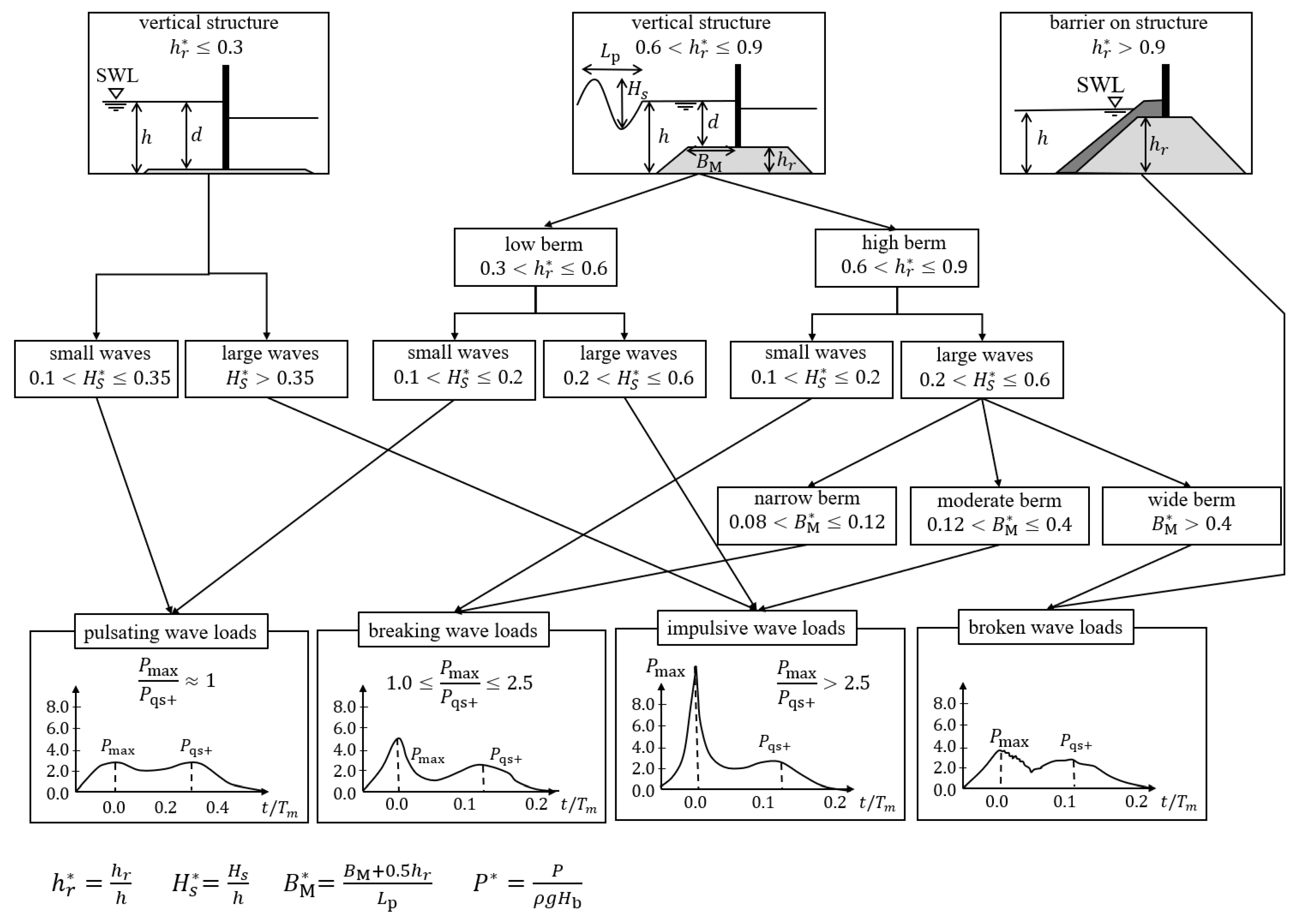
2.2. Wave Loading Types

Kortenhaus and Oumeraci [12] distinguish between four different wave loading types. An overview of their time-histories and generation mechanism is shown in Figure 1. The figure includes depth-induced breaking waves only. The following wave loading types are distinguished:

• Pulsating wave loads are gently varying forces due to the reflection of windwaves of low to medium steepness on a vertical wall. Typical wave periods are in the order of $T_{\mathrm{m}}=1-25$ s [13].
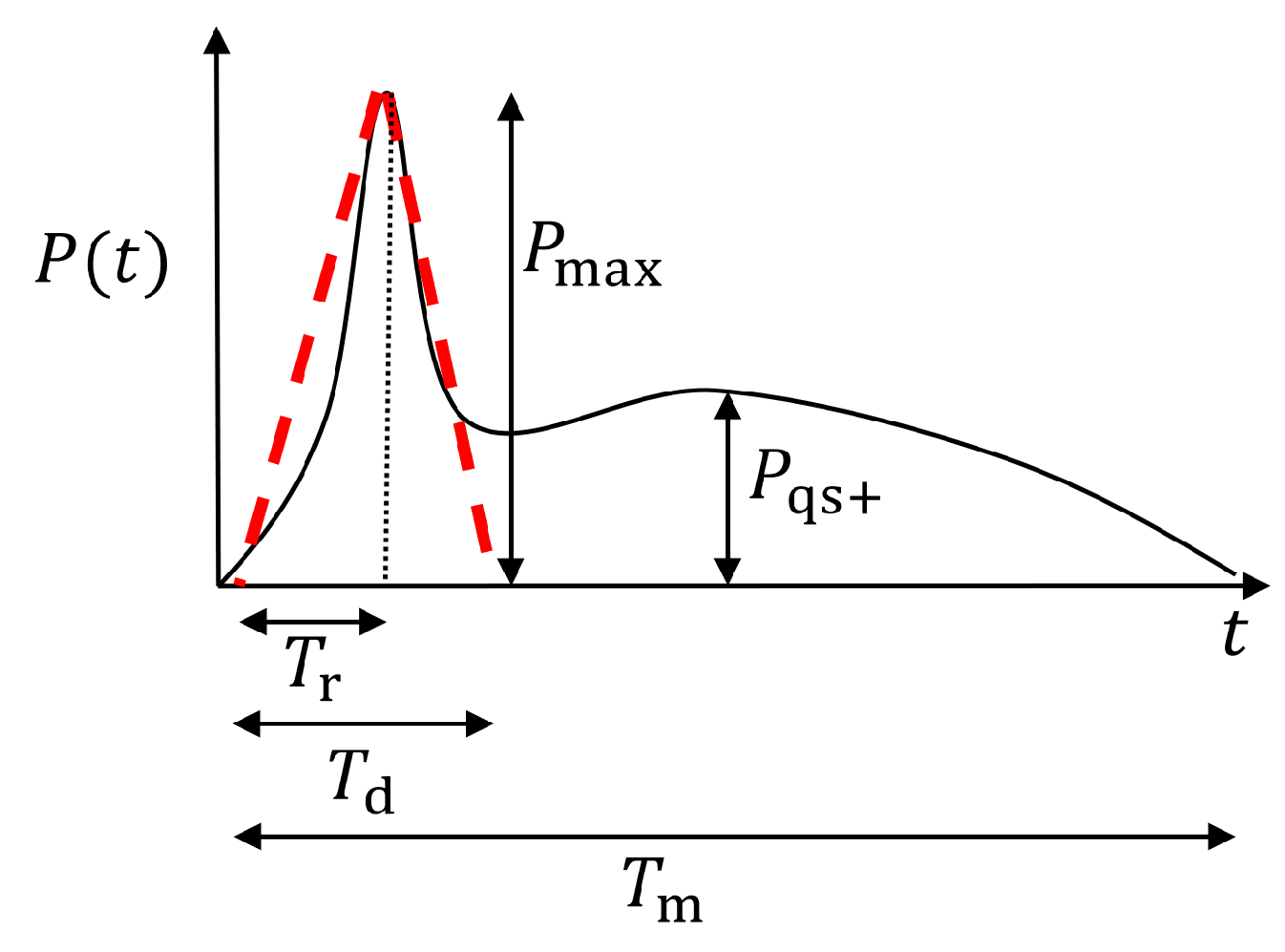
• (Slightly) breaking and impulsive wave loads occur when the incoming wave is high as compared to the water depth, combined with a steep sea-bottom or the presence of a rubble mound. The time-histories of breaking or impulsive wave loads consists of two components; a first peak of relatively short duration ($P_{\max }$), followed by a second, (s)lower wave peak ($P_{\mathrm{qs}+}$) with duration around the mean wave period $T_{\mathrm{m}}$ (see also Section 3.2.1). The typical duration of the peak lies between $T_{\mathrm{d}}=$ 0.01–0.2 s with rise times between $T_{\mathrm{r}}=$ 0.1–30 ms, see e.g., [14,15,16]. For (slightly) breaking and impulsive wave loads the ratio between the maximum and quasi-static peak lies between $1\le P_{\max }/P_{\mathrm{qs}+}\le 2.5$. For impact wave loads it lies above $P_{\max }/P_{\mathrm{qs}+}>2.5$. There exists a strong (negative) dependency between the loading magnitude $P_{\max }/P_{\mathrm{qs}+}$ and the duration of the peak $T_{\mathrm{d}}$, see [15,17].
• Post breaking waves occur when the waves break before they hit the structure. Their load history resembles that for slightly breaking wave loads. However, the presence of a large air content induces aerial damping which slightly decreases the magnitude and duration of the first breaking peak.

Both slender hydraulic structures and caisson structures typically have a quasi-static response to pulsating wave loads, and a dynamic response to breaking or impact wave loads (see Section 2.3 and Section 2.4). In the assessment of the applicability of GT to slender hydraulic structures it is therefore distinguished between pulsating wave loads on the one hand, and breaking and impact wave loads on the other hand (see Section 3).

2.3. Dynamic Characteristics of Slender Hydraulic Structures

Slender hydraulic structures come in all shapes and sizes. Their appearance varies from relatively simple plate-like structures of moderate dimensions (for example a glass plate as part of a water retaining wall [18], a splash barrier on top of a sea wall [11], or a small sluice gate as presented in Figure 2) to large elastic multi-structures composed of a number of structural elements such as plates, beams, and trusses (see for example the storm surge barriers presented in Figure 3 and Figure 4). Popular materials are steel, concrete, timber, or glass, which behave more or less linear elastic under normal circumstances. Due to their plain and slender nature, uplift wave loads are typically small. As they often consist of many components, slender hydraulic structures are assessed on both global (e.g., support reactions) and local failure mechanisms (e.g., cross-sectional assessment of components). Especially for the assessment of local failure mechanisms, a detailed description of the wave pressures over the height and width of the structure is needed.

The dynamic behavior of slender hydraulic structures depends on many factors, among which the dimensions of the structure or structural element, the structural boundary conditions (free, simply supported, clamped, etc.), the stiffness of the joints, and the material properties (modulus of elasticity, mass density, lateral contraction coefficient, etc.). A crucial aspect regards the influence of the fluid–structure interaction, which depends on the water level(s) surrounding the structure.

Several approaches exist to model the dynamic behavior of slender hydraulic structures subjected to wave loads [1]. These approaches range from relatively simple Single Degree Of Freedom (SDOF) analyses to the application of advanced 3D time-history analyses including fluid–structure interaction, non-linear material behavior, and complex geometries (typically conducted using finite element models). An insightful way of describing the dynamic behavior of slender hydraulic structures is modal analysis. Thereby the vibration of the structure is thought of as the summation of a number of separate (independent) modes that each vibrate in their own (3D) mode shapes and frequencies (see also Section 3.4). Not all modes contribute equally much to the total dynamic behavior of the structure. Which modes contributes most depends on aspects like the loading duration as compared to the modal frequency, the shape of the pressure distribution, and the modal damping.

A wide variety of slender hydraulic structures and structural elements exists in practice. Therefore also a wide variety of natural frequencies can be expected in practice. As a reference, Chen et al. [15] estimated a representative range of natural periods between 0.02 s and 0.5 s (2–50 Hz). This means that most hydraulic structures have characteristic natural periods much shorter than the mean wave period, but much longer than the characteristic duration of the breaking and impact wave loads. As a result, slender hydraulic structures typically have a quasi-static response to pulsating wave loads, and a dynamic response to breaking and impact wave loads.

The likelihood of encountering a certain wave loading type strongly depends on the type of structure under consideration. Water regulating structures like sluices or navigation locks are typically installed in sheltered areas such as (man-made) channels or behind breakwaters. They therefore typically encounter small, or low steepness waves. As one of their main functions is to ensure sufficient water depth (e.g., for shipping purposes), they are often positioned in relatively deep waters. Figure 1 shows that these conditions typically lead to pulsating wave loads, on which the structures are expected to have a quasi-static response. A typical example of this kind is the navigation lock in IJmuiden, The Netherlands [19].

On the other hand, there exist slender hydraulic structures with a purpose of flood or splash protection, such as splash guards [11] or storm-surge barriers [15], that operate during heavy storms with high wind-induced waves. These structures are sometimes positioned on a berm or steep sea-bed. Figure 1 shows that these type of structures are therefore more likely to be loaded by heavily breaking or impact wave loads, on which the structures are expected to have a dynamic response.

2.4. Dynamic Characteristics of Caisson Structures

Caisson breakwaters are designed to ensure calm waters behind them. They are heavy monolithic structures whose dynamic system is strongly determined by the mass of the caisson and the non-linear soil conditions of the sea-bed and rubble mound. They often consist of a vertical caisson structure on the one hand, and a rubble mound on the other hand. As they operate in open seas, they are subjected to all types of wave loads; from pulsating wave loads during calm seas to heavily breaking or impact wave loads during severe storms.

Vertical caisson breakwaters are typically assessed on the global sliding and overturning failure mechanisms only. Thereby both horizontal and uplift (or buoyancy) wave loads may play an important role. The main focus of their design is directed towards the adequate prediction of resultant forces and moments at the caisson base. The accurate description of wave pressures over the height and width of the structure is of lesser importance.

Several models exist to describe the dynamic system of caisson structures, of which an overview is provided in Cuomo et al. [17]. The vast majority of the models regard (analytical) N-Degree Of Freedom (NDOF) models [21,22,23,24,25], of which a selection is shown in Figure 5. Wave loads are typically modeled as horizontal point-loads at the location of the momentum center. The vertical wave loads are often disregarded, as they are slower or out phase with the horizontal wave loads (see for example Goda [26]).

Cuomo et al. [16] estimated the natural periods of several caisson breakwaters, and found values between 0.15 s and 2 s (0.5–6.7 Hz). According to Allsop et al. [8], Goda’s original wave load formula corresponds to caissons with natural periods between 0.1 and 0.3 s (3.3–10 Hz). This means that most caisson structures have characteristic natural periods much shorter than the mean wave period, but around or much longer than the duration of the impact or breaking peak. Caisson structures are therefore expected to have a quasi-static response to pulsating wave loads, and a dynamic response to breaking and impact wave loads.

2.5. Background on Goda–Takahashi Wave Load Formula

The GT wave load formula was primarily derived for the assessment of the sliding and overturning failure mechanisms of caisson breakwaters. To assess the applicability of GT to other structural types and failure mechanisms, it is thus important to know what the modeling assumptions were in its derivation, and how these relate to the deviating design situations. For this we performed a literature study on the historical backgrounds of GT, which is presented in Section 2.5.2. For convenience we first present the formulations of GT in Section 2.5.1.

2.5.1. Formulation of the GT Wave Load Formula

The GT wave load formula was derived in several stages and by several authors. The final version of the formula is presented in Goda [3], where distinction is made between ‘Goda’s original load formula’ and ‘Takahashi’s extensions’.

Goda’s Original Wave Load Formula

Goda’s original wave load formula was derived by Goda in [27,28]. It was later adjusted by Tanimoto [29] to account better for oblique wave attack, and by Takahashi et al. [30,31] and Kamikubo et al. [11] to account better for different wall types and shapes via modification factors (${\lambda }_i$). The assumed pressure distribution is presented in Figure 6. The ‘horizontal’ pressure intensity follows a trapezoidal shape between still water level ($p_1$), the sea bottom ($p_2$), and the top of the wave run-up ($\eta$). The ‘uplift’ pressure intensity is distributed triangularly between the seaward edge ($p_3$) to zero at the rear heal. The shape of the distribution is assumed not to change under any condition (wave type, the presence of a rubble mound, wave over-topping, etc.). In case of plain, vertical caisson structures the expressions for the wave run-up $\eta$ and pressure intensities $p_1,p_2,p_3$ are:

$$\begin{array}{cc}\hfill \eta & =0.75(1+cos\beta )H_{\mathrm{D}}\hfill \\ \hfill p_1& =0.5(1+cos\beta )\left({\alpha }_1+{\alpha }_2{cos}^2\beta \right)w_0{H}_{\mathrm{D}}\hfill \\ \hfill p_2& =\frac{p_1}{cosh\left(2\pi h/L_{\mathrm{D}}\right)}\hfill \\ \hfill p_3& ={\alpha }_3{p}_1\hfill \end{array}\begin{array}{cc}\hfill {\alpha }_1& =0.6+0.5{\left[\frac{4\pi h/L_{\mathrm{D}}}{sinh(4\pi h/L_{\mathrm{D}})}\right]}^2\hfill \\ \hfill {\alpha }_2& =min\left[\frac{1}{3}\left(1-\frac{d}{h_{\mathrm{b}}}\right){\left(\frac{H_{\mathrm{D}}}{d}\right)}^2,\frac{2d}{H_{\mathrm{D}}}\right]\hfill \\ \hfill {\alpha }_3& =1-\frac{h^{\prime }}{h}\left(1-\frac{1}{cosh(2\pi h/L_{\mathrm{D}})}\right)\hfill \end{array}$$

(5)

where ${\alpha }_1$ represents the pressure coefficient accounting for the slowly-varying (quasi-static) wave component, ${\alpha }_2$ the additional peak for the breaking wave component, h the design water depth at the seaward rubble mound base, $h_{\mathrm{b}}$ the design water depth at a distance five times the design significant wave height seawards from the structure, d the design water depth above the rubble mound, $\beta$ the incident wave direction, $w_0$ the specific weight of the water, $H_{\mathrm{D}}$ the design wave height as determined by formulae provided in Goda [28], $L_{\mathrm{D}}$ the design wave length, and $h^{\prime }$ the design water depth at the caisson base. In case of vertical slender hydraulic structures placed in (man-made) channels, it often holds $h^{\prime }=d$ and $\theta \approx 0$.

Takahashi’s Extensions

Takahashi et al. [32,33] found that Goda’s original wave load formula did not under all conditions adequately predicted the equivalent-static pressures under impulsive wave loads. They therefore extended Goda’s original wave load formula to better account for impact loads caused by wave breaking on the rubble mound. The modification is applied by changing ${\alpha }_2$ in Equation (5) to ${\alpha }^{*}=max\left([{\alpha }_2,{\alpha }_{\mathrm{I}}]\right)$ with:

$$\begin{array}{ccc}\hfill {\alpha }_{\mathrm{I}}& ={\alpha }_{\mathrm{I}0}{\alpha }_{\mathrm{I}1}\hfill & \\ \hfill {\alpha }_{\mathrm{I}0}& =min\left[H/d,2\right]\hfill & \\ \hfill {\alpha }_{\mathrm{I}1}& =\left\{\begin{array}{cc}cos\left({\delta }_2\right)/cosh\left({\delta }_1\right)\hfill & :{\delta }_2\le 0\hfill \\ 1/\left(cosh\left({\delta }_1\right)\sqrt{cosh\left(\delta 2\right)}\right)\hfill & :{\delta }_2>0\hfill \end{array}\right.\hfill \end{array}\begin{array}{cc}\hfill {\delta }_1& =min(20{\delta }_{11},15{\delta }_{11})\hfill \\ \hfill {\delta }_2& =min(4.9{\delta }_{22},3.0{\delta }_{22})\hfill \\ \hfill {\delta }_{11}& =0.93(B_{\mathrm{M}}/L_{\mathrm{D}}-0.12)+0.36(0.4-d/h)\hfill \\ \hfill {\delta }_{22}& =-0.36(B_{\mathrm{M}}/L_{\mathrm{D}}-0.12)+0.93(0.4-d/h)\hfill \end{array}$$

(6)

where ${\alpha }_{\mathrm{I}}$ represents the ‘impulsive’ pressure coefficient, ${\alpha }_{\mathrm{I}0}$ entails the effect of wave height, and ${\alpha }_{\mathrm{I}1}$ entails the effect of the mound width ($B_{\mathrm{M}}$).

2.5.2. Derivation of the Wave Load Formulae

Goda’s Original Wave Load Formula

Goda’s original wave load formula relies on a large number of experimental and theoretical considerations reported in various Japanese reports. The English summaries of these reports are understandably compressed and do not describe all steps in the derivation process. Based on some personal conversations with experienced persons in the field, combined with the available English and Japanese reports, a reconstruction of the derivation of the wave load formula could be made.

(1)

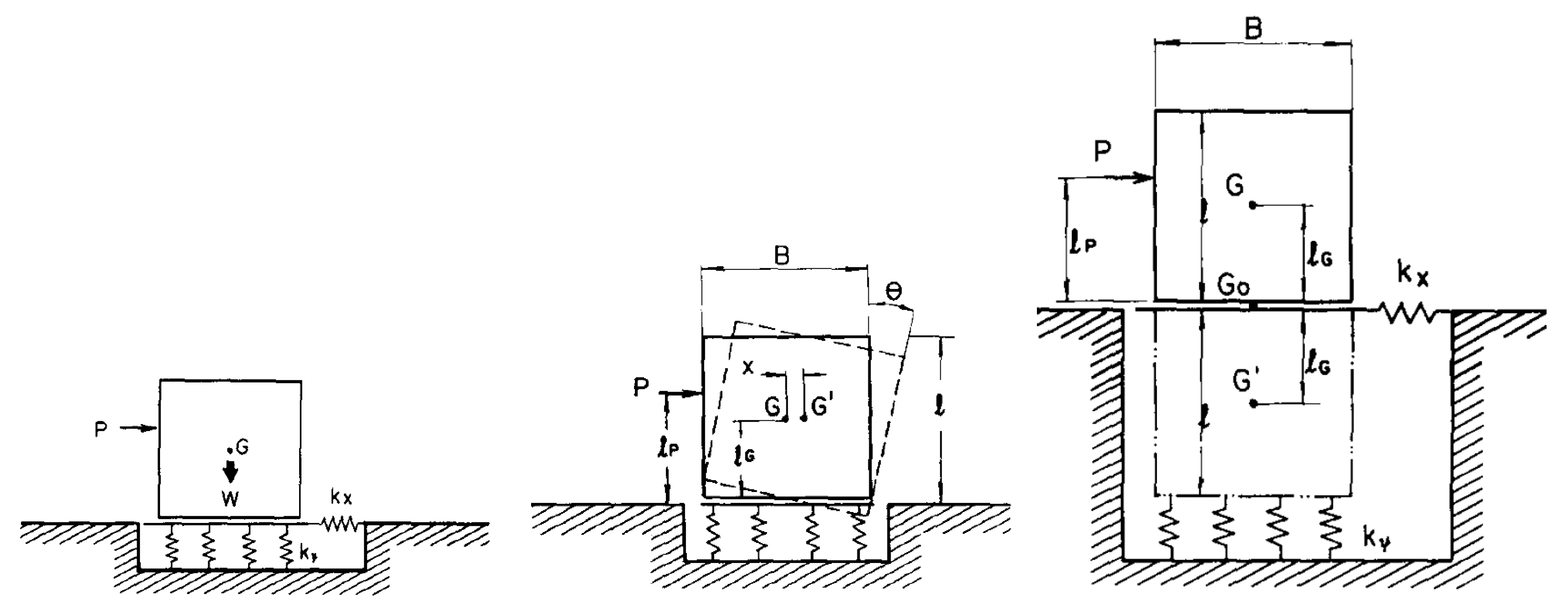
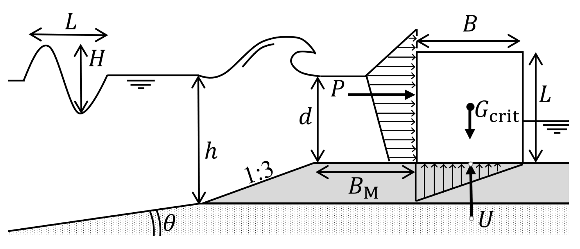
In the early 1970s, Goda conducted a large number of sliding experiments of which the supposed experimental set-up is visualized in Figure 7. A model caisson breakwater with self-weight G was positioned in a wave flume on a rubble mound with (known) friction coefficient $\mathsf{\mu }$. At the beginning of the wave flume a (regular) test wave was generated. When the wave reached the structure, it exerted a (time-dependent) horizontal $P\left(t\right)$ and uplift $U\left(t\right)$ wave load on it. Next, the critical caisson weight $G_{\mathrm{crit}}$ was determined for which just no sliding occurred. This was then used to calculate the corresponding equivalent-static wave loads by Coulombs friction law: $P_{\mathrm{eq},\mathrm{sliding}}=\mathsf{\mu }(G_{\mathrm{crit}}-U_{\mathrm{eq}})$. For this step, an estimate was made on the effective uplift forces $U_{\mathrm{eq}}$, of which the details are unknown. In the experiments, a large number different wave heights, wave periods, water levels, and mound heights were considered.

(2)

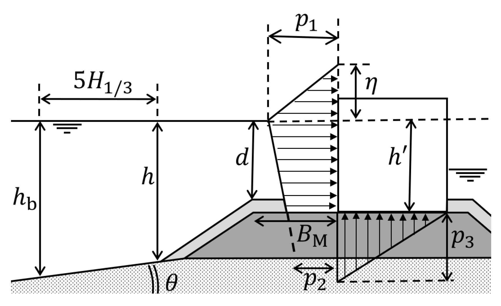
In 1972, Goda performed a smaller number of experiments in a wave flume where horizontal and uplift wave pressures were measured using pressure transducers [34,35]. Different wave heights, wave periods, water levels, and mound heights were considered. Both pulsating, (slightly) breaking, or post-breaking waves were included (regular waves only). Together with theoretical considerations on fourth-order standing wave theory from Goda [36], an idealized shape of the incoming wave pressure distribution was derived such as described by Equation (5).

(3)

Given the equivalent-static wave loads derived in step (1), and the idealized shape of the pressure distribution from step (2), Goda subsequently back-calculated the values of $p_1,p_2,p_3,\eta$ to empirically fit the results from the sliding experiments. This resulted in the final expressions for ${\alpha }_1,{\alpha }_2,{\alpha }_3$. About this derivation Goda [28] stated: “The results of the experiments [...] as well as the requirement of simplicity in the application of formulae have brought the author to propose the distribution of design wave pressure [...]. The pressure factors of ${\alpha }_1$ and ${\alpha }_2$ have been determined empirically on the basis of experimental data and the calibration of new formulae with the case studies of prototype breakwaters. [...]. Though the agreement between the formulae and the laboratory data is not excellent, the difference may be disregarded for the purpose of general formulation of wave pressure estimation”.

(4)

After the formula was derived it was calibrated against case-studies from real breakwater failures during heavy seas, see Goda [28]. It is not entirely clear to the authors of this study if this calibration was used for validation purposes only, or whether it was also used to update the previously derived model from step (3).

Most likely some additional aspects have played a role as well. In a discussion on the derivation of effective wave loads Takahashi et al. [37] state: “the standard way [...] is to first establish the pressure formula for the impact pressure on the wall, and then formulate a theoretical dynamic model of the dynamic response to calculate the effective pressure. [...]. The Goda pressure formula was basically formulated via this procedure”. What theoretical dynamic model Takahashi et al. [37] refer to, or how this information was taken into account, is not explicitly mentioned. Possibly Goda’s dynamic caisson model presented in [26,38] was used for this purpose.

Goda [28] does not mention the dynamic characteristics of the considered caisson structures in scope of the sliding experiments from step (1). According to Allsop et al. [8] the caissons considered by Goda had natural periods around 0.1 to 0.3 s. It should however be remarked that for a given set of incoming wave characteristics GT predicts a single value for the equivalent-static wave loads only, regardless of the exact natural period of the caisson structure under consideration. This means that in the derivation of the model a certain ’representative’ natural period of the caissons must have been chosen.

Takahashi’s Extensions

The derivation of Takahashi’s impulsive pressure coefficient followed more or less the same steps (1) and (3) as Goda. The sliding experiments were however performed by Tanimoto et al. [39], and were designed such that impact wave loads due to the wave breaking on the rubble mound were generated. The exact dynamic properties of the model caissons could not be retrieved. It is however expected that the natural periods of the caissons considered by Tanimoto et al. [39] are roughly within the same range as those considered by Goda, because the experiments were performed at the same facilities of the Port and Harbor Research Institute of Japan.

In the derivation of Takahashi’s extensions the actual shape of the wave pressure distribution in step (2) was not considered. Main reason for this is that Takahashi’s extensions were never intended to accurately predict wave pressures over the height of the structure (nor to accurately predict wave loads for that matter). The main purpose of the impulsive pressure coefficient was to indicate the risk of high impulsive wave loads, such that this information could be used to adapt the design of the structure.

2.6. Model Uncertainties in GT

This study investigates the applicability of GT for the assessment of slender hydraulic structures. Naturally, this applicability depends on the error we make when GT is applied to slender hydraulic structures. This error may emerge from difference causes. In the following paragraphs we therefore briefly discuss the different sources of errors, or ’model uncertainties’, inherent to GT, and how they can be quantified.

2.6.1. Different Sources of Model Uncertainties

Model uncertainties quantify the difference between a model’s prediction and reality [40]. In the application of GT to slender hydraulic structures, three sources of model uncertainties can be distinguished:

• Type (a) model uncertainties represent the uncertainties related to the lack of knowledge about the detailed interplay between the considered variables [40]. GT was derived empirically on the basis of a limited number of experiments including scaled model caissons and regular waves. It is however known that scaled wave loads do not fully represent reality [16], and neither do regular waves. Moreover, only a limited number of design situations was investigated and potentially important design situations may have been overlooked.
• Type (b) model uncertainties arise from the fact that the derivation of any model is guided by the balance between its ability to represent reality and the pragmatic need for simplicity and generality [40]. It was discussed in Section 2.5.2 that also in the derivation of Goda’s original wave load formula “requirements of simplicity” and “general formulation” have played an important role. Aspects that are for example deliberately ignored are: (i) the influence of wave over-topping on the pressure intensity at the height of the structure, or (ii) the influence of wave loading type on the shape of the pressure distribution, or (iii) the frequency-dependency of the caisson structures on the equivalent-static wave loads.
• The last type of model uncertainties is related to the application of a model outside of its intended scope. Reasons for this are either the lack of knowledge (no better model is available) or the need for simplicity (a more appropriate model is available but we choose to apply the less adequate model nonetheless). This inadequate application of the model introduces additional uncertainties which are referred to as type (c) model uncertainties. GT was derived to predict equivalent-static wave loads for the sliding and overturning failure mechanism of caisson breakwaters with natural periods between 0.1–0.3 s. It was not derived for the cross-sectional assessment of slender hydraulic structures with natural periods between 0.02 and 0.5 s. When applying GT to slender hydraulic structures it is thus clearly applied outside of its intended dynamic scope. The magnitude of the resulting type (c) uncertainties depends on the extent to which dynamic aspects play a role. In case of pulsating wave loads the type (c) uncertainties will be small, as both caissons and hydraulic structures will have a quasi-static response. In case of breaking or impact loads on hydraulic structures however the type (c) uncertainties become larger, as the dynamic response can differ.

This means that in case of pulsating wave loads the application of GT to slender hydraulic structures leads to type (a) and (b) model uncertainties only, whereas in case of breaking or impact wave loads additional type (c) model uncertainties are introduced.

2.6.2. Quantification of Model Uncertainties

There are several ways to investigate the model uncertainties inherent to GT for slender hydraulic structures. The most straightforward approach would be to perform a large number of experimental (laboratory) studies on slender hydraulic structures loaded by waves, and continuously measure the dynamic response $R_{\mathrm{dyn}}\left(t\right)$. Via Equations (1) and (2) then the maximum dynamic response $R_{\mathrm{dyn},\max }$ can be obtained and ’translated’ to the equivalent-static wave loads $P_{\mathrm{eq},R}$. The obtained value $P_{\mathrm{eq},R}$ can then be compared to the equivalent-static wave loads predicted by GT Equations (5) and (6). This approach provides direct insights in the combination of type (a), (b) and (c) uncertainties together. It would however be interesting to know the impact of the ’additional’ type (c) uncertainties in relation to the already present type (a) and (b) uncertainties. In the following section we therefore adopt an alternative approach, which quantifies the type (c) uncertainties separately.

3. Methodology

3.1. Bird-Eye Overview

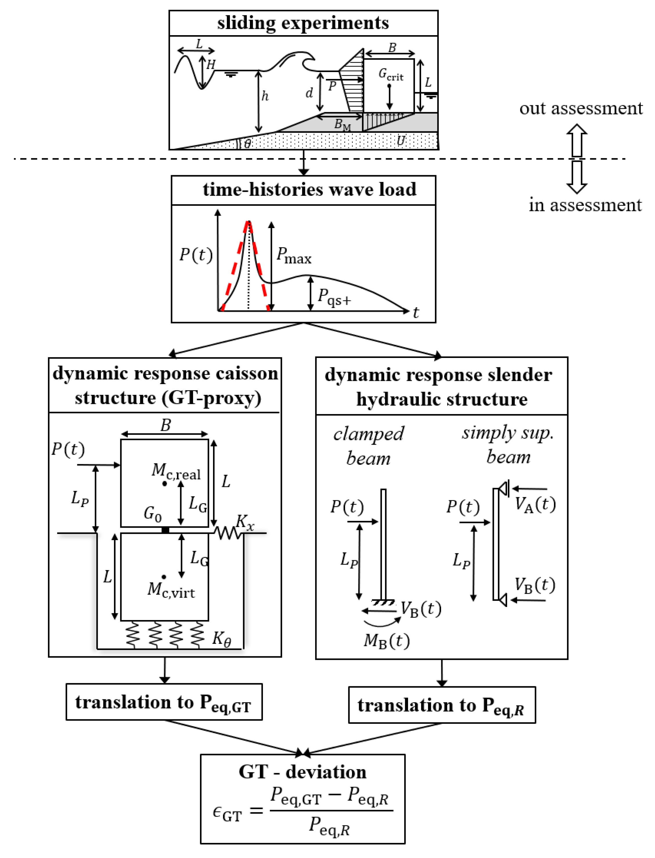
The idea behind the approach is as follows. In the derivation of GT the dynamic behavior of the caisson structures was captured by the sliding experiments from step (1) in Section 2.5.2. If similar experiments would have been conducted for slender hydraulic structures, this would naturally have resulted in different equivalent-static wave loads and therefore different predictions by GT. The (hypothetical) difference between the equivalent-static wave loads from the caisson sliding experiments on the one hand, and the slender hydraulic structures on the other hand, is thus a measure for the model uncertainties of type (c) only. In the approach we therefore aim at (analytically) mimicking the sliding experiments from step (1), whereby we additionally investigate the dynamic behavior of the slender hydraulic structures (see Figure 8). The differences in obtained equivalent-static wave loads for the caissons on the one hand, and the slender hydraulic structures on the other hand, then serves as a proxy for the type (c) model uncertainties related to the application of GT to slender hydraulic structures. The approach consists of the following steps:

(1)

First step is to attain a representative time-histories of an incoming wave load $P\left(t\right)$ such as occurred within the sliding experiments. The exact generation mechanism behind this incoming wave load (such as the incoming wave dimensions, mound dimensions, etc.) is assumed to be known. For details on the wave load modeling see Section 3.2.

(2)

Based on an analytic dynamic model we then mimic the dynamic behavior of the caisson breakwater at base shear and quantify the corresponding equivalent-static wave loads ($P_{\mathrm{eq},\mathrm{GT}}$). The obtained value for $P_{\mathrm{eq},\mathrm{GT}}$ then serves as a proxy for the equivalent-static wave loads as derived in the GT-sliding experiments. This is reasonable as long as: (i) the incoming wave load profiles resemble those underlying the GT-sliding experiments and ($ii$) the analytic dynamic caisson model adequately describes the dynamic behavior of the model caissons within the GT-sliding experiments. This step is further elaborated in Section 3.3.

(3)

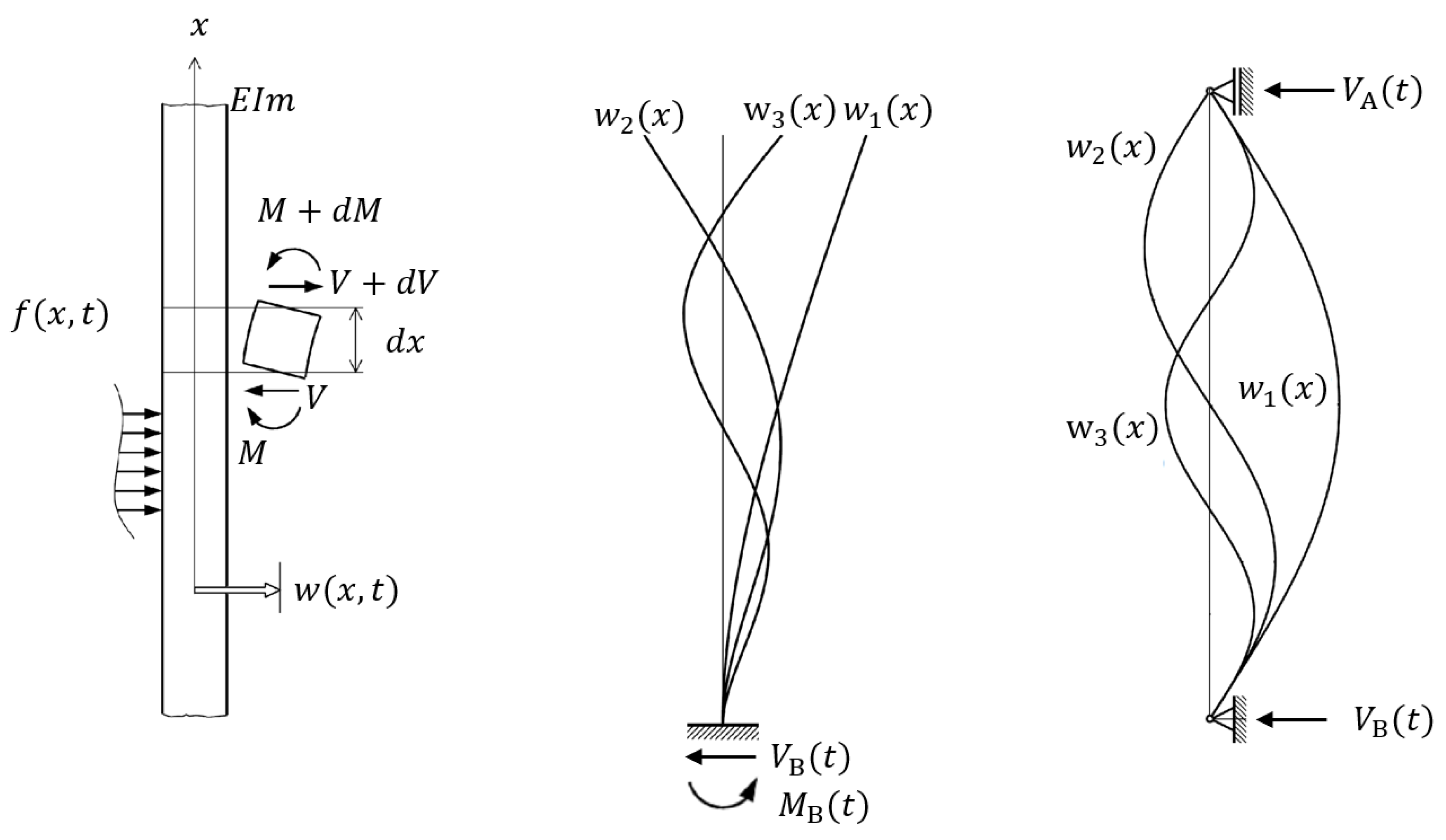
Next, the equivalent-static wave loads for two typical slender hydraulic structures subjected to the same incoming wave load $P\left(t\right)$ are determined. Two structural types are considered. The first is a 2D clamped plate whereby interest goes to the loads at base shear ($V_{\mathrm{B}}$) and base moment ($M_{\mathrm{B}}$). The second is a 2D simply supported plate whereby interest goes to top shear ($V_{\mathrm{A}}$) and bottom shear ($V_{\mathrm{B}}$). The clamped plate represents for example a typical splash-guard on top of a flood wall [11], and the simply supported plate represents for example the main beams of a rolling gate. This step is further elaborated in Section 3.4.

(4)

The difference in dynamic behavior is now referred to as the ’GT-deviation’ and is determined by:

$${ϵ}_{\mathrm{GT}}=\frac{P_{\mathrm{eq},\mathrm{GT}}-P_{\mathrm{eq},R}}{P_{\mathrm{eq},R}}·100\%$$

(7)

where $P_{\mathrm{eq},\mathrm{GT}}$ is the proxy for the equivalent-static wave loads as obtained during the GT-sliding experiments and $P_{\mathrm{eq},R}$ the equivalent-static wave load for the slender hydraulic structure subjected to the same incoming wave load.

3.2. Time-Histories of Incoming Wave Load

3.2.1. Church-Roof Wave Load Model

The incoming horizontal wave load is modeled as a single point-load $P\left(t\right)$ located at the height of the momentum center $L_P$. The vertical wave load is disregarded in the assessment, which was found to be common practice for both the caisson structures and slender hydraulic structures in dynamic assessments (see Section 2.4 and Section 2.3). The time-histories of the horizontal wave load is modeled according to the idealized church-roof shape by Oumeraci and Kortenhaus [25], which has been favored by many authors in the past, see e.g., [15,16] and Figure 9. In the literature however many other (more advanced) models exist as well, of which an overview is given in Cuomo et al. [17]. The expression for the church-roof wave load is:

$$P\left(t\right)=\left\{\begin{array}{cc}{P}_{\max }\frac{t}{T_{\mathrm{r}}}\hfill & :t\le T_{\mathrm{r}}\hfill \\ P_{\max }\left(1-\frac{t-T_{\mathrm{r}}}{T_{\mathrm{d}}-T_{\mathrm{r}}}\right)\hfill & :T_{\mathrm{r}}<t\le T_{\mathrm{d}}\hfill \\ 0\hfill & :t>T_{\mathrm{d}}\hfill \end{array}\right.$$

(8)

where $P_{\max }$ represents the breaking wave peak, $T_{\mathrm{r}}$ the rise time, and $T_{\mathrm{d}}$ the total impact duration.

It is remarked that the horizontal wave loads are simplified as resultant forces with a certain moment arm only. In case of slender hydraulic structures this simplification is not entirely correct, as the shape of the pressure distribution influences the dynamic response via expression (25), see later. The study however focuses on highly breaking or impact wave loads only, for which the peak pressure intensity is highly concentrated around the point of the impact location, see e.g., [41]. The simplifications are therefore expected to be sufficiently accurate for the purpose of this study.

3.2.2. Correction for Quasi-Static Part of the Wave Load

The church-roof wave load model from Oumeraci and Kortenhaus [25] considers the breaking peak ($P_{\max }$) only and does not account for the quasi-static part of the wave load ($P_{\mathrm{qs}+}$). In reality however the response of the structure is a function of the breaking ($P_{\max }$) and the quasi-static ($P_{\mathrm{qs}+}$) part combined. To account for this aspect a practical approach suggested by Chen et al. [15] is adopted, which assumes that the total equivalent-static wave load ($P_{\mathrm{eq},R}$) can be constructed by the summation of the response to the quasi-static part of the wave load ($P_{\mathrm{qs}+}$) and the church-roof part of the wave load ($P_{\max }$). Since $P_{\mathrm{qs}+}$ is assumed within the static loading domain of the structure, the equivalent-static wave load for reaction force R caused by this part of the load is equal to $P_{\mathrm{qs}+,\mathrm{eq},R}=P_{\mathrm{qs}+}$. The reaction force to the church-roof part of the wave load is then determined by a dynamic analysis such as described in the following subsections. Following this methodology, the equivalent-static reaction force to the total incoming wave load is expressed by:

$$\begin{array}{cc}\hfill P_{\mathrm{eq},R}& =P_{\mathrm{qs}+}+P_{\mathrm{eq},R}^{*}\hfill \end{array}$$

(9)

where $P_{\mathrm{eq},R}^{*}$ represents the equivalent-static wave load corresponding to the church-roof part of the wave load. Using Equation (4) the Equation (9) can also be written as:

$$P_{\mathrm{eq},R}=P_{\mathrm{qs}+}+{\mathrm{DLF}}_R^{*}{P}_{\max }$$

(10)

Although the method is merely an approximation, it was found to be in good agreement with the theoretically correct values for SDOF systems [15].

3.2.3. Investigated Wave Loads

In the study, the following wave load characteristics are investigated (see also

Table 1. Overview of input parameters adopted in this study.

Description	Symbol	Value (s)
Investigated wave loads $P\left(t\right)$
relative moment-arm wave load	$L_P/L$	0.3, 0.6, 0.8
impact loading duration	$T_{\mathrm{d}}$	0.01–0.2 s
relative rise time	$T_{\mathrm{r}}/T_{\mathrm{d}}$	0.5
relative impulsive magnitude
- (slightly) breaking wave loads	$P_{\max }/P_{\mathrm{qs}+}$	1–2.5
- impact wave loads	$P_{\max }/P_{\mathrm{qs}+}$	2.5-10
Caisson structures (proxy for GT caissons)
relative caisson width	$B/L$	1.25
relative center of gravity	$L_G/L$	0.5
ratio horizontal and rotational period of vibration	$T_{\theta }/T_x$	0.94
range of horizontal period of vibration	$T_x$	0.1–0.3 s *
Slender hydraulic structures
range of first modal period of vibration	$T_{n=1}$	0.05–2 s

* Values are summarized into a single representative value via Equation (21).

).

• Relative moment-arm ($L_P/L$): The value of the relative moment arm is highly depending on the design situation under consideration (wave height, period, water level, etc.). Since the GT-sliding experiments contained a whole range of wave dimensions, water levels, and mound heights, it is expected that relative moment arms from high to low were represented in the experiments. In this study, we investigate the ratios $L_P/L=[0.3,0.6,0.8]$.
• Impact duration ($T_{\mathrm{d}}$): The GT-sliding experiments embodied the whole range from slowly pulsating to heavily breaking or impact wave loads. It was found that typical impact durations were between 0.01–0.2 s (see Section 2.2) and it is expected that such orders of magnitude were embodied by the GT experiments as well. In this study, we therefore investigate the whole range of impact durations between $T_{\mathrm{d}}=0.01-0.2s$.
• Relative rise time ($T_{\mathrm{r}}/T_{\mathrm{d}}$): Depending on the breaker type in front of the caisson breakwater (flip through, vertical wave front, or plunging wave) different ratios for the rise time and total impact duration $T_{\mathrm{r}}/T_{\mathrm{d}}$ are observed in practice, see Cuomo et al. [42]. It is unknown what breaker types occurred during the GT-sliding experiments. In case no further information is provided, Cuomo et al. [16] suggest a symmetrical pulse shape ($T_{\mathrm{r}}/T_{\mathrm{d}}=0.5$). This value is adopted in this study as well.
• Relative impact magnitude ($P_{max}/P_{\mathrm{qs}+}$): The GT-sliding experiments contained the whole range from pulsating to highly impulsive wave loads. It can thus be expected that the whole range of impact magnitudes between roughly $1<P_{\max }/P_{\mathrm{qs}+}\le 10$ have occurred. In analogy with the wave classification by Kortenhaus and Oumeraci [12] we distinguish between relative impact magnitudes corresponding to breaking wave loads ($1<P_{\max }/P_{\mathrm{qs}+}\le 2.5$) and impact magnitudes corresponding to impact wave loads ($2.5<P_{\max }/P_{\mathrm{qs}+}<10$).

It should be noted that not all investigated loading situations are equally likely to be observed in practice. For example high impact loads ($P_{\max }/P_{\mathrm{qs}+}$) are more likely to occur with short impact duration ($T_{\mathrm{d}}$) as was also discussed in Section 2.2. Moreover, higher moment-arms ($L_P/L$) are more likely to occur than low moment-arms, for reasons that slender hydraulic structures are often designed such that over-topping is allowed.

3.3. Equivalent-Static Wave Loads for the GT-Sliding Experiments

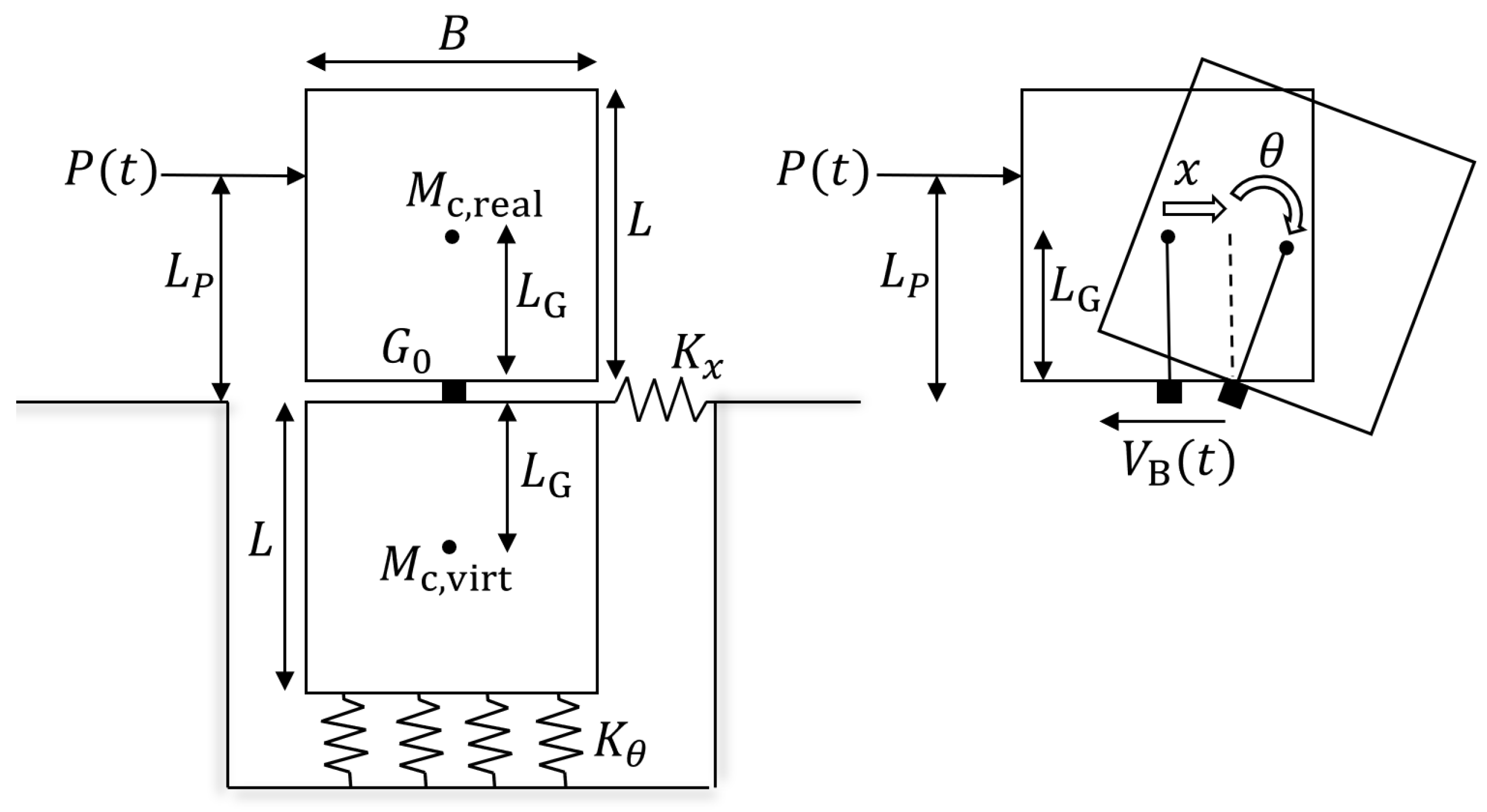
3.3.1. Analytic Dynamic Model

The dynamic behavior of the caissons is modeled on the basis of the analytic dynamic caisson model by Goda [26,38], see Figure 10. The motivation for this model is twofold. Firstly, it was found to adequately predict the sliding behavior of caisson structures. Secondly, it may have been used in the derivation of Goda’s original wave load formula (see Section 2.5.2).

Goda’s dynamic caisson model [26,38] has two degrees of freedom: the horizontal translation x and rotational displacement $\theta$. The caisson is represented as an effective mass $M_{\mathrm{c},\mathrm{real}}$ with dimensions $B\ast L$. The mass includes both the caisson mass and the added water mass, and acts at the center of gravity $L_G$. At the friction surface $G_0$ the mass is connected to a second, virtual mass $M_{\mathrm{c},\mathrm{virt}}$, which represents the effective mass of the rubble mound and foundation. The virtual mass is connected to a horizontal and rotational spring with stiffness per unit width:

$$K_x=K_x^{*}B,K_{\theta }=(1/12)K_{\theta }^{*}{B}^3$$

(11)

where $K_x^{*},K_{\theta }^{*}$ are the coefficients of soil reaction for the translational and rotational vibration. For the virtual mass Goda chooses $M_{\mathrm{c},\mathrm{virt}}=M_{\mathrm{c},\mathrm{real}}$, which is adopted in this study as well. Damping of the soil is not accounted for. As long as the shear force at $G_0$ does not exceed the friction, the real and virtual mass move together with total mass $M_{\mathrm{c}}=M_{\mathrm{c},\mathrm{real}}+M_{\mathrm{c},\mathrm{real}}$. This system is described by the following equations of motion:

$$\begin{array}{cc}\hfill & M_{\mathrm{c}}\ddot{x}\left(t\right)+K_{x}x\left(t\right)=P\left(t\right)\hfill \\ \hfill & M_{\mathrm{c}}(r_0^2+L_G^2)\ddot{\theta }\left(t\right)+K_{\theta }\theta \left(t\right)=L_{P}P\left(t\right)\hfill \end{array}$$

(12)

where $r_0^2=(B^2+L^2)/12$ describes the radius of gyration of the mass about its center of gravity. The solution to the church-roof part of the wave load $P\left(t\right)$ is given by [26]:

$$x\left(t\right)=\left\{\begin{array}{cc}\frac{P_{\max }}{M_{\mathrm{c}}}\left(\frac{t}{{\omega }_x^3{T}_{\mathrm{r}}}-\frac{sin\left({\omega }_{x}t\right)}{{\omega }_x^3{T}_{\mathrm{r}}}\right)\hfill & :t\le T_{\mathrm{r}}\hfill \\ \frac{P_{\max }}{M_{\mathrm{c}}{\omega }_x^3}\left(sin\left({\omega }_x(t-T_{\mathrm{r}})\right)\left(\frac{1}{T_{\mathrm{r}}}+\frac{1}{T_{\mathrm{d}}-T_{\mathrm{r}}}\right)-\frac{sin\left({\omega }_{x}t\right)}{T_{\mathrm{r}}}+\frac{{\omega }_x(T_{\mathrm{d}}-t)}{T_{\mathrm{d}}-T_{\mathrm{r}}}\right)\hfill & :T_{\mathrm{r}}\le t\le T_{\mathrm{d}}\hfill \\ \frac{P_{\max }}{M_{\mathrm{c}}{\omega }_x^3}\left(sin\left({\omega }_x(t-T_{\mathrm{r}})\right)\left(\frac{1}{T_{\mathrm{r}}}+\frac{1}{T_{\mathrm{d}}-T_{\mathrm{r}}}\right)-\frac{sin\left({\omega }_{x}t\right)}{T_{\mathrm{r}}}-\frac{sin\left({\omega }_x(t-T_{\mathrm{d}})\right)}{T_{\mathrm{d}}-T_{\mathrm{r}}}\right)\hfill & :t\ge T_{\mathrm{d}}\hfill \end{array}\right.$$

(13)

and for the rotational vibration:

$$\theta \left(t\right)=\left\{\begin{array}{cc}\frac{P_{\max }}{M_{\mathrm{c}}(r_0^2+L_G^2)}\left(\frac{t}{{\omega }_{\theta }^3{T}_{\mathrm{r}}}-\frac{sin\left({\omega }_{\theta }t\right)}{{\omega }_{\theta }^3{T}_{\mathrm{r}}}\right)\hfill & :t\le T_{\mathrm{r}}\hfill \\ \frac{P_{\max }}{M_{\mathrm{c}}(r_0^2+L_G^2){\omega }_{\theta }^3}\left(sin\left({\omega }_{\theta }(t-T_{\mathrm{r}})\right)\left(\frac{1}{T_{\mathrm{r}}}+\frac{1}{T_{\mathrm{d}}-T_{\mathrm{r}}}\right)-\frac{sin\left({\omega }_{\theta }t\right)}{T_{\mathrm{r}}}+\frac{{\omega }_x(T_{\mathrm{d}}-t)}{T_{\mathrm{d}}-T_{\mathrm{r}}}\right)\hfill & :T_{\mathrm{r}}\le t\le T_{\mathrm{d}}\hfill \\ \frac{P_{\max }}{M_{\mathrm{c}}(r_0^2+L_G^2){\omega }_{\theta }^3}\left(sin\left({\omega }_{\theta }(t-T_{\mathrm{r}})\right)\left(\frac{1}{T_{\mathrm{r}}}+\frac{1}{T_{\mathrm{d}}-T_{\mathrm{r}}}\right)-\frac{sin\left({\omega }_{\theta }t\right)}{T_{\mathrm{r}}}-\frac{sin\left({\omega }_{\theta }(t-T_{\mathrm{d}})\right)}{T_{\mathrm{d}}-T_{\mathrm{r}}}\right)\hfill & :t\ge T_{\mathrm{d}}\hfill \end{array}\right.$$

(14)

with natural frequencies:

$${\omega }_x=\sqrt{K_x/M_{\mathrm{c}}}{\omega }_{\theta }=\sqrt{K_{\theta }/\left(M_{\mathrm{c}}(r_0^2+L_G^2)\right)}$$

(15)

3.3.2. Input-Parameters

The dynamic behavior of the caissons is defined by the following parameters:

• Relative caisson width ($B/L$): The exact geometric characteristics of the caisson structures in scope of the GT-sliding experiments are unknown. The dimensions of the real-life caisson structures analyzed by Goda [28] in step (4) of Section 2.5.2 were however between $B/L=0.65-1.5$. A sensitivity study showed that within this range the exact value of $B/L$ had little influence on the dynamic response. In this study, therefore the value of $B/L=1.25$ is adopted, for reasons that this value was also taken in Goda [26].
• Relative caisson center of gravity ($L_G/L$): Caisson structures are often designed as rectangular concrete boxes filled with (more or less) homogeneous soil. A reasonable value for the relative center of gravity therefore seems $L_G/L=0.5$. Small deviations from this value were found to have little influence on the results and were not further investigated. The value $L_G/L=0.5$ was also taken in Goda [26].
• Ratio rotational and horizontal period of vibration ($T_x/T_{\theta }$): The ratio between the rotational and horizontal period of vibration is captured by Equations (11) and (15) and can be expressed by:

  $${\omega }_{\theta }/{\omega }_x=T_x/T_{\theta }=\sqrt{K_x^{*}/K_{\theta }^{*}\frac{1/12\left({(B/L)}^2+1\right)+{(L_G/L)}^2}{1/12{(B/L)}^2}}$$

  (16)
  Since the values for the relative caisson width ($B/L$) and relative center of gravity ($L_G/L$) are known, the ratio $T_x/T_{\theta }$ depends on the choice for $K_x^{*}/K_{\theta }^{*}$ only. It is unknown what soil properties were used during the GT-sliding experiments. Goda [26] adopted the value $K_x^{*}/K_{\theta }^{*}=0.25$, which is adopted in this study as well. Substituting the chosen values for $B/L=1.25$, $L_G/L=0.5$ and $K_x^{*}/K_{\theta }^{*}=0.25$ into Equation (16) leads to the fixed ratio $T_x/T_{\theta }=0.94$. This means that the horizontal and rotational degree of freedom vibrate in more or less the same natural period.
• Natural period of horizontal vibration ($T_x$): According to Allsop et al. [8] the caissons in scope of Goda’s original wave load formula had natural periods between 0.1 and 0.3 s. It is not mentioned to which degree of freedom these natural periods correspond to. Since both degrees of freedom were found to vibrate in more or less the same period ($T_x/T_{\theta }=0.94$), the exact choice is of minor importance and the horizontal degree of freedom x was taken.

3.3.3. Equivalent-Static Wave Loads for Base Shear

Interest goes to the dynamic response at base-shear $V_{\mathrm{B},\mathrm{dyn}}\left(t\right)$, which can be calculated as the difference between the incoming wave load $P\left(t\right)$ and the horizontal components of the inertia forces, see Figure 10:

$$V_{\mathrm{B},\mathrm{dyn}}\left(t\right)=P\left(t\right)-M_{\mathrm{c},\mathrm{real}}(\ddot{x}+L_G\ddot{\theta })$$

(17)

The maximum dynamic response is evaluated for a period as long as the duration of the wave impact ($T_{\mathrm{d}}$) and a single ‘free’ period of horizontal vibration ($T_{\mathrm{x}}$):

$$V_{\mathrm{B},\mathrm{dyn},\max }=max{\left[V_{\mathrm{B},\mathrm{dyn}}\left(t\right)\right]}_{T_{\mathrm{d}}+T_x}$$

(18)

No longer period is investigated, as from hereon it is expected that damping starts playing a significant role—decreasing the dynamic response. Using Equation (2) the corresponding equivalent-static wave load can be determined by:

$$P_{\mathrm{eq},\mathrm{sliding}}^{*}=V_{\mathrm{B},\mathrm{dyn},\max }$$

(19)

where the asterisk indicates the fact that it corresponds to the church-roof part of the wave load only. Correction of the quasi-static part of the wave load by Equations (9) and (10) leads to:

$$\begin{array}{cc}\hfill P_{\mathrm{eq},\mathrm{sliding}}& =P_{\mathrm{qs}+}+P_{\mathrm{eq},\mathrm{sliding}}^{*}\hfill \\ \hfill & =P_{\mathrm{qs}+}+{\mathrm{DLF}}_{\mathrm{sliding}}^{*}{P}_{\max }\hfill \end{array}$$

(20)

It was discussed before that for a given set of incoming wave characteristics GT predicts a single value for the equivalent-static wave loads only, regardless of the exact natural period of the caisson structure under consideration. We should thus ’summarize’ our obtained equivalent-static wave loads into a single, representative value. It is unknown what this representative value corresponds to (mean value, envelope value, median value). For the purpose of this study we assume that it corresponds to the unweighted average over the equivalent-static wave loads $P_{\mathrm{eq},\mathrm{sliding}}$ as obtained over the range of caisson periods $T_{\mathrm{x}}$ = 0.1–0.3, i.e.,

$$P_{\mathrm{eq},\mathrm{GT}}=\mu {\left(P_{\mathrm{eq},\mathrm{sliding}}\right)}_{T_{\mathrm{x}}\in [0.1-0.3]s}$$

(21)

where $\mu (.)$ stands for the mean value and $P_{\mathrm{eq},\mathrm{GT}}$ for the proxy of the equivalent-static wave loads obtained by the GT sliding experiments. It is noted that a different definition for $P_{\mathrm{eq},\mathrm{GT}}$ leads to different estimates of the GT-deviation. The differences are however expected to be small, for reasons that otherwise (most likely) a frequency–dependency would have been introduced into the GT wave load formula.

3.4. Analytic Dynamic Models for Slender Hydraulic Structures

3.4.1. Analytic Dynamic Model

The slender hydraulic structures are modeled as 2D Euler–Bernoulli beams with flexural stiffness $EI$ and equally distributed mass m. This effective mass is assumed to include an (equally distributed) added water mass such as determined by more advanced methods as presented in e.g., [1,43]. The equations of the transverse motion of the Euler–Bernoulli beam are given by [44]:

$$EI\frac{{\delta }^{4}w(x,t)}{\delta x^4}+m\frac{{\delta }^{2}w(x,t)}{\delta t^2}=I\left(x\right)P\left(t\right)$$

(22)

with $I\left(x\right)=0$ for $x\ne L_P$ and $I\left(x\right)=1$ for $x=L_P$. Structural damping is thus not accounted for in the analysis. Equation (22) is solved using modal analysis, where the beam displacement $w(x,t)$ is taken as a summation over n modes with modal shapes $w_n\left(x\right)$ and modal amplitudes $q_n\left(t\right)$:

$$w(x,t)=\sum _{n=1}^N{w}_n\left(x\right)q_n\left(t\right)$$

(23)

where N stands for the number of modes, for which we take $N=10$. The solutions for the modal shapes and frequencies are presented in

Table 2. Modal frequency and shape for clamped and simply supported beam with ${\omega }_0={\left(\frac{\pi }{L}\right)}^2\sqrt{\frac{EI}{m}}$ [44].

	Clamped	Simply Supported
modal frequency	${\omega }_1={0.6}^2{\omega }_0$, ${\omega }_n=\frac{1}{2}{\omega }_0$	${\omega }_n=n^2{\omega }_0$
modal shape	$A_n\left(\frac{cosh\left({\beta }_{n}x\right)-cos\left({\beta }_{n}x\right)}{cosh\left({\beta }_{n}L\right)+cos\left({\beta }_{n}L\right)}-\frac{sinh\left({\beta }_{n}x\right)-sin\left({\beta }_{n}x\right)}{sinh\left({\beta }_{n}L\right)+sin\left({\beta }_{n}L\right)}\right)$	$A_{n}sin\left(\frac{n\pi x}{L}\right)$
	with ${\beta }_1=0.6\frac{\pi }{L}$, ${\beta }_n=\left(1-\frac{1}{2}\right)\frac{\pi }{L}$

and Figure 11. The solution to the modal amplitude is given by (expressions derived by the author):

$$q_n\left(t\right)=\left\{\begin{array}{cc}\frac{P_n}{M_n}\left(\frac{t}{{\omega }_n^3{T}_{\mathrm{r}}}-\frac{sin\left({\omega }_{n}t\right)}{{\omega }_n^3{T}_{\mathrm{r}}}\right)\hfill & :t\le T_{\mathrm{r}}\hfill \\ \frac{P_n}{M_n{\omega }_n^3}\left(sin\left({\omega }_n(t-T_{\mathrm{r}})\right)\left(\frac{1}{T_{\mathrm{r}}}+\frac{1}{T_{\mathrm{d}}-T_{\mathrm{r}}}\right)-\frac{sin\left({\omega }_{n}t\right)}{T_{\mathrm{r}}}+\frac{{\omega }_n(T_{\mathrm{d}}-t)}{T_{\mathrm{d}}-T_{\mathrm{r}}}\right)\hfill & :T_{\mathrm{r}}\le t\le T_{\mathrm{d}}\hfill \\ \frac{P_n}{M_n{\omega }_x^3}\left(sin\left({\omega }_n(t-T_{\mathrm{r}})\right)\left(\frac{1}{T_{\mathrm{r}}}+\frac{1}{T_{\mathrm{d}}-T_{\mathrm{r}}}\right)-\frac{sin\left({\omega }_{n}t\right)}{T_{\mathrm{r}}}-\frac{sin\left({\omega }_n(t-T_{\mathrm{d}})\right)}{T_{\mathrm{d}}-T_{\mathrm{r}}}\right)\hfill & :t\ge T_{\mathrm{d}}\hfill \end{array}\right.$$

(24)

with the modal mass ($M_n$), stiffness ($K_n$), load ($P_n$), and frequency (${\omega }_n$) given by: 2

$$\begin{array}{cc}\hfill M_n& =m\underset{0}{\overset{L}{\int }}{w}_n^2\left(x\right)\mathrm{d}x\hfill \\ \hfill K_n& =EI\underset{0}{\overset{L}{\int }}{w}_n^2\left(x\right)\frac{{\delta }^4{w}_n\left(x\right)}{\delta x^4}\mathrm{d}\hfill \end{array}$$

$$\begin{array}{cc}\hfill P_n& =\underset{0}{\overset{L}{\int }}{w}_n\left(x\right)f(x,t)\mathrm{d}x\hfill \\ \hfill {\omega }_n& =\sqrt{K_n/M_n}\hfill \end{array}$$

(25)

3.4.2. Equivalent-Static Wave Loads for Reaction Force R

The internal shear and moment in the Euler-Bernoulli beams are obtained by [44]:

$$V(x,t)=-EI\frac{{\delta }^{3}w(x,t)}{\delta x^3}$$

(26)

$$\begin{array}{c}\hfill M(x,t)=-EI\frac{{\delta }^{2}w(x,t)}{\delta x^2}\end{array}$$

(27)

In case of the clamped beam interest goes to the dynamic reaction force at base shear $V_{\mathrm{B},\mathrm{dyn}}\left(t\right)$ and base moment $M_{\mathrm{B},\mathrm{dyn}}\left(t\right)$. These are obtained by substituting $x=0$ into Equations (26) and (27) respectively and accounting for the equilibrium. In case of the simply-supported beam, interest goes to top shear $V_{\mathrm{A},\mathrm{dyn}}$(t) and bottom shear $V_{\mathrm{B},\mathrm{dyn}}\left(t\right)$. These are obtained by substituting $x=L$ and $x=0$ in Equation (26) and accounting for the equilibrium. The maximum dynamic response is evaluated for the period as long as the duration of the impact load ($T_{\mathrm{d}}$) and the first natural period of the structure ($T_{n=1}$):

$$R_{\mathrm{dyn},\max }=max{\left[R_{\mathrm{dyn}}\left(t\right)\right]}_{T_{\mathrm{d}}+T_{n=1}}$$

(28)

whereby $R_{\mathrm{dyn}}\left(t\right)$ represents either one of the reaction forces of the clamped or simply supported beam. No longer time-frame is investigated, as from here-on it is expected that damping starts to play a significant role. The equivalent-static wave loads to reaction force R are obtained by:

$$P_{\mathrm{eq},R}^{*}=f_{P\to R}^{-1}\left(R_{\mathrm{dyn},\max }\right)$$

(29)

where the asterisk denotes the fact that it corresponds to the church-roof part of the wave load only. Correction of the quasi-static part of the wave load by Equations (9) and (10) leads to:

$$\begin{array}{cc}\hfill P_{\mathrm{eq},R}& =P_{\mathrm{qs}+}+P_{\mathrm{eq},\mathrm{R}}^{*}\hfill \\ \hfill & =P_{\mathrm{qs}+}+{\mathrm{DLF}}_R^{*}{P}_{\max }\hfill \end{array}$$

(30)

3.4.3. Considered Natural Periods

For a given set of incoming wave characteristics, the dynamic response of the slender hydraulic structures is uniquely defined by their first natural period ($T_{n=1}$) only. This value is highly structure dependent, as was discussed in Section 2.3. To gain a good general overview, the whole range between $T_{n=1}$ = 0.05–2 s was investigated.

4. Results

For each set of incoming wave load characteristics and for each support reaction R, the GT-deviation was determined according to the methodology described in the previous section. Before investigating the results, we first take a closer look at the dynamic response to the church-roof part of the wave load only, as this lays on the basis of the GT-deviations and provides valuable insights. In Section 4.1 the time-histories of a single (church-roof) design situation is presented. In Section 4.2 a summary of all other (church-roof) design situations is presented. Section 4.3 presents the resulting GT-deviations for a large number of case-studies. The results were validated with Abaqus Non-Linear Finite Element Analysis (SIMULIA).

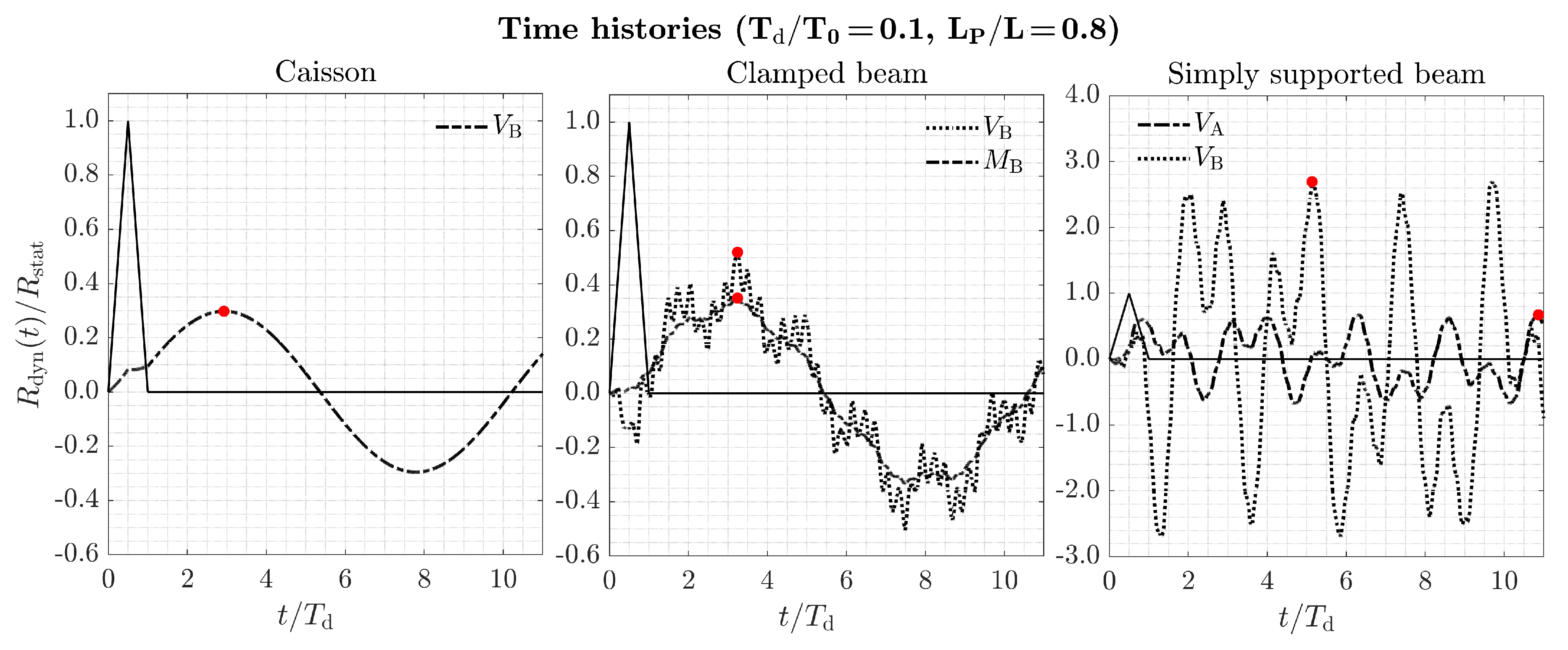
4.1. Time-Histories of Reaction Forces for Representative (Church-Roof) Design Situation

Figure 12 shows the time-histories of the dynamic support reactions for the caisson structure (left), clamped beam (middle), and simply supported beam (right) subjected to a wave load with moment arm $L_P/L=0.8$ and impact duration $T_{\mathrm{d}}=0.01$ s (for all other input parameters see Table 1). The characteristic natural periods of the caisson and slender hydraulic structure used the same value $T_0=T_x=T_{n=1}=0.1$ s. The static reaction force is presented by a black-solid line. All other lines represent the resulting dynamic responses. The red dots indicate the maximum dynamic response over the considered period of time. For convenience, all reaction forces $R_{\mathrm{dyn}}\left(t\right)$ are normalized with their static equivalent $R_{\mathrm{stat}}$. The values denoted by the red dots therefore correspond to the dynamic load factor DLF${}_R^{*}$.

Caisson structure: In the case of the caisson structure the dynamic reaction at base shear first increases up to the value of $V_{\mathrm{B},\mathrm{dyn}}\left(t\right)/V_{\mathrm{B},\mathrm{stat}}\approx 0.1$, then remains more or less constant, and then attains a smooth, sinusoidal vibration with period around $T\approx 0.1$ s. The dynamic load factor is equal to ${\mathrm{DLF}}_{\mathrm{sliding}}^{*}\approx 0.3$, meaning that the caisson structure behaves impulsively on the church-roof part of the wave load.

Clamped beam: For the clamped beam the dynamic response of the base shear ($V_{\mathrm{B}}$) is presented as a dotted line and the dynamic response of the base moment ($M_{\mathrm{B}}$) as a dashed line. The obtained DLF for the base moment is equal to ${\mathrm{DLF}}_{M_{\mathrm{B}}}^{*}\approx 0.35$ and the obtained DLF for the base shear is equal to ${\mathrm{DLF}}_{V_{\mathrm{B}}}^{*}\approx 0.52$. Both support reactions thus have impulsive behavior. For both support reactions the free vibration is dominated by the first modal period of $T_{n=1}=0.1$, yet with some additional, high-frequent components superposed.

Simply supported beam: For the simply supported beam the dynamic response of the lower support reaction ($V_{\mathrm{B}}$) is presented as a dotted line and the dynamic response of the upper support reaction ($V_{\mathrm{A}}$) as a dashed line. The obtained DLF for the upper support reaction is equal to ${\mathrm{DLF}}_{V_{\mathrm{A}}}^{*}\approx 0.7$ and the obtained DLF for the lower support reaction is equal to ${\mathrm{DLF}}_{V_{\mathrm{B}}}^{*}\approx 2.7$. The dynamic amplification of the lower support reaction ($V_{\mathrm{B}}$) is significantly higher than for the upper support reaction ($V_{\mathrm{A}}$). This is related to the elevation level at which the load is applied (see also next Section 4.2). For both the upper and lower support reaction four peaks are observed in the free vibration with intermediate period $\Delta T\approx 0.025$ s. This period corresponds to the second vibration mode of the structure, as can be obtained by the formulas in Table 2 with $n=2$. The relative importance of this second vibration mode is attributed to the fact that relative moment-arm $L_P/L=0.8$ lies closely to the point of maximum deflection for the considered mode shape, which lies at $L_P/L=0.75$ (see Figure 11).

Damping: In case of the slender hydraulic structures, the negligence of damping is clearly visible. As a result, the total dynamic response of the slender hydraulic structures is slightly over-estimated. For example, in the case of the simply supported beam and the upper support reaction ($V_{\mathrm{A}}$), the maximum dynamic response occurs around time $t/T_{\mathrm{d}}=10$. In reality however the second mode ($n=2$) would probably have damped out here already to a certain extent, and the actual maximum dynamic response would thus have been somewhere before $t/T_{\mathrm{d}}<10$ (most likely somewhere around the first two ‘free’ vibrations of the second mode, so between $t/T_{\mathrm{d}}=1-4$). It is however expected that the difference in obtained DLFs is relatively small, as can be obtained from the figure as well.

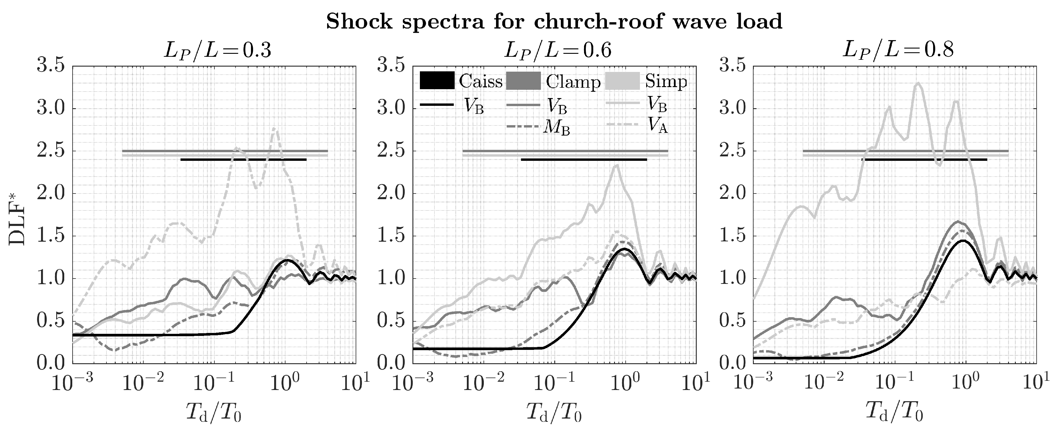
4.2. Dynamic Load Factors for All Other Design Situations (Shock-Spectra)

The same analysis is conducted for all other design situations. The results are summarized in Figure 13, which presents the obtained dynamic load factors as a function of impact loading duration ($T_{\mathrm{d}}$) as compared to the characteristic natural period of the structure ($T_0=T_x=T_{n=1}$). For each structure the ‘range of interest’ is indicated by a horizontal line. For caisson structures this range of interest lies between $T_{\mathrm{d}}/T_x\in 0.033-2.0$ and for the slender hydraulic structures between $T_{\mathrm{d}}/T_{n=1}\in 0.005-4.0$ (see Table 1). The presented DLFs for the caisson structures correspond to the equivalent-static wave loads as obtained by Equation (19). It is noted that the DLFs as obtained in the example of Section 4.1 can be found from Figure 13 as well.

The obtained DLFs differ greatly from structure to structure and from support reaction to support reaction. Some clear (expected) patterns are however observed. Regardless of the structure or support reaction, for $T_{\mathrm{d}}/T_0>5$ the response converges towards the quasi-static loading domain and for $T_{\mathrm{d}}/T_0\to 0.001$ towards the impulsive loading domain. For loading duration around $T_{\mathrm{d}}/T_0\approx 1$ the dynamic response is most pronounced, with DLFs sometimes far above 1.

Caisson structure: The shock spectra of the caisson structure follow a smooth pattern, and the dynamic behavior rapidly moves into the impulsive loading domain. Already for values around $T_{\mathrm{d}}/T_0<0.1$ the obtained DLFs systematically lie below $0.5$; a behavior which is also expected from the multitude of references investigating the impulsive behavior of caisson structures subjected to wave impacts, see e.g., [32]. For values $T_{\mathrm{d}}/T_0\to 0$ the shock spectra converge to a constant value not equal to zero. This is related to the adopted analytic description of the caisson model (see Section 3.3), for which it can be derived that this lower-bound converges to ${\mathrm{DLF}}_{\mathrm{caisson}}^{*}=1/2-\left(L_P{L}_G\right)/\left(2(r_0^2+L_G^2)\right)$.

Clamped beam: The DLFs for the base shear ($V_{\mathrm{B}}$) and base moment ($M_{\mathrm{B}}$) are presented as solid and dashed lines respectively. The results for the base moment ($M_{\mathrm{B}}$) show great similarities with the ones obtained for the caisson structure; this especially holds for $L_P/L=0.8$. In case of the base shear ($V_{\mathrm{B}}$) however the results deviate from the caisson structure, and starting from $T_{\mathrm{d}}/T_0<0.3$ systematically higher DLFs are obtained.

Simply supported beam: The DLFs for the lower support reaction ($V_{\mathrm{B}}$) and upper support reaction ($V_{\mathrm{A}}$) are presented in solid and dashed lines respectively. The ‘dynamic sensitivity’ of the simply supported beam is much larger than for the other structural types. DLFs up to the value of 3.3 are obtained, see for example $L_P/L=0.8$ and $0.1<T_{\mathrm{d}}/T_0\le 1$. A remarkable difference with the other structural types is the pronounced sensitivity of the obtained DLFs to the moment-arm $L_P/L$. The DLFs for the lower support reaction ($V_{\mathrm{B}}$) systematically increase with increasing moment-arm, whereas the DLFs for the upper support reaction ($V_{\mathrm{A}}$) systematically decrease with increasing moment-arm. This behavior will come back in the results for the GT-deviation as well (see Figure 15).

4.3. Investigation of the GT-Deviation

Figure 14 and Figure 15 show the obtained GT-deviations for the clamped and simply supported beam as a function of relative moment-arm ($L_P/L$), impact loading duration ($T_{\mathrm{d}}$), impact magnitude ($P_{\max }/P_{\mathrm{qs}+}$) and natural period of the structure ($T_{n=1}$). The values for $1\le P_{\max }/P_{\mathrm{qs}+}\le 2.5$ are presented as a range corresponding to the breaking wave load type, and the values for $2.5\le P_{\max }/P_{\mathrm{qs}+}\le 10$ are presented as a range corresponding to the impact wave load type. For brevity the results for impact duration $T_{\mathrm{d}}=[0.01,0.05,0.1,0.2]$ s are presented only. The gray horizontal lines demarcate the GT-deviations above or below 25%. GT-deviations above ${ϵ}_{\mathrm{GT}}>0$ indicate an over-estimation of the equivalent-static wave loads for reaction force R and GT-deviations below ${ϵ}_{\mathrm{GT}}<0$ indicate an under-estimation of the equivalent-static wave loads for reaction force R.

The results strongly depend on the considered design situation, and it is difficult to establish clear patterns. They will be further discussed for the clamped and simply supported beam separately. It is remarked that not all design situations are equally likely to be observed in practice, as was discussed previously in the paper as well.

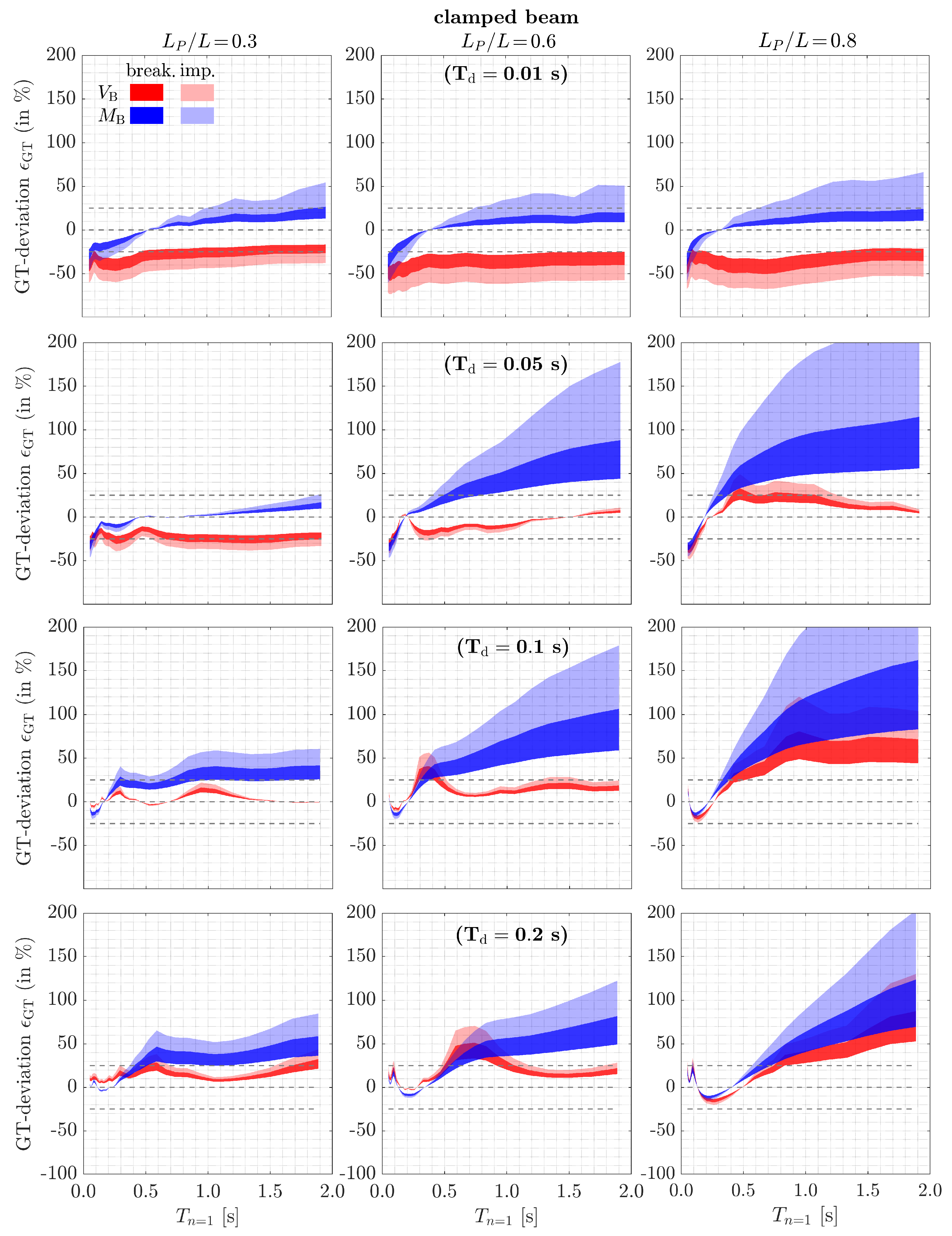
4.3.1. GT-Deviations for the Clamped Beam

The GT-deviations for the clamped beam are presented in Figure 14. The values for the base shear ($V_{\mathrm{B}}$) are presented in red and the values for the base moment ($M_{\mathrm{B}}$) are presented in blue. In case of the base shear ($V_{\mathrm{B}}$) and for the shorter loading duration ($T_{\mathrm{d}}=0.01$ s and $T_{\mathrm{d}}=0.05$ s) the vast majority of the design situations has GT-deviations below ${ϵ}_{\mathrm{G}\mathrm{T}}<0$. Under-estimations up to 50% are observed for breaking wave loads, and over 50% for impact wave loads. For the longer loading duration ($T_{\mathrm{d}}=0.1$ s and $T_{\mathrm{d}}=0.2$ s) the vast majority of the design situations have GT deviations above ${ϵ}_{\mathrm{G}\mathrm{T}}>0$. Over-estimations up to 60% are observed for breaking wave loads, and over 100% for impact wave loads. In case of base moment ($M_{\mathrm{B}}$) and natural periods below $T_{n=1}<0.5$ s, the vast majority of the design situations lies within $-25\%<{ϵ}_{\mathrm{GT}}\le 25\%$. For increasing natural periods $T_{n=1}>0.5$ s, systematic over-estimations are obtained, with GT-deviations over 100% in case of breaking wave loads and over 200% in case of impact wave loads (see for example $T_{\mathrm{d}}=0.05$, $L_P/L=0.8$ and $T_{n=1}>1.5$ s). For both support reactions the GT-deviations increase with increasing natural period $T_{n=1}$. This positive tendency is explained by the fact that the model caissons from the GT-sliding experiments had natural periods between 0.1 and 0.3 s only, whereas for the slender hydraulic structures natural periods up to $T_{n=1}=2$ s are investigated; for natural periods above $T_{n=1}>0.3$ s thus not only the differences in structural system between the caisson and slender hydraulic structure play a role, but also the differences in natural frequencies as well.

4.3.2. GT-Deviations for the Simply Supported Beam

The GT-deviations for the simply supported beam are presented in Figure 15. The values for the lower support ($V_{\mathrm{B}}$) are presented in blue and for the upper support reaction ($V_{\mathrm{A}}$) in red. In case of the lower support reaction ($V_{\mathrm{B}}$) the vast majority of the design situations has GT-deviations below ${ϵ}_{\mathrm{G}\mathrm{T}}<0$. Under-estimations up to 80% are observed for breaking wave loads and over 90% for impact wave loads, see for example $T_{\mathrm{d}}=0.01$ s and $L_P/L=0.8$. Similar values are found for the upper support reaction ($V_{\mathrm{A}}$). For some design situations GT-deviations above ${ϵ}_{\mathrm{GT}}>0$ are observed, with values up to 50% for breaking waves and up to 90% for impact wave loads (see $T_{\mathrm{d}}=0.05$ s and $L_P/L=0.8$). Similar as for the clamped beam, the GT-deviations slightly increase with increasing natural period $T_{n=1}$. This tendency is however weaker than for the clamped beam, for reasons that the differences in dynamic behavior and natural periods between the model caissons and the simply supported beam cancel each other out to a certain extent.

5. Discussion

5.1. Comparison of Model Uncertainties

This study investigates the applicability of GT for slender hydraulic structures. This applicability depends on the error we make when GT is applied to slender hydraulic structures. In Section 2.6 we distinguished between three sources of model uncertainties: those related to a lack of knowledge (type a); those related to deliberate simplifications (type b); those related to its application outside of its dynamic domain (type c). In the previous section, a first estimate on the type (c) uncertainties was gained for a number of design situations (see Figure 14 and Figure 15). The following paragraphs discuss how the additional type (c) uncertainties relate to the already present type (a) and (b) uncertainties.

5.1.1. Model Uncertainties Related to Lack of Knowledge and Deliberate Simplifications-Type (a) and (b)

Several experimental and numerical studies quantified the type (a) and (b) model uncertainties in relation to caisson structures, see e.g., [9,11,42,45,46,47,48,49]. Probably the most extended studies were those performed by Meer et al. [45,46], who quantified model uncertainties in Goda’s original wave load formula on the basis of a large number of experiments carried out at several hydraulic institutes. The experiments comprised different caisson dimensions and shapes, foreshore conditions, mound dimensions, and hydraulic loading conditions. In total, 134 data sets were investigated for the horizontal forces and moments, and 31 for the uplift wave forces and moments. The model uncertainty was defined by:

$${\chi }_{\mathrm{ab}}=\frac{P_{\mathrm{measured}}}{P_{\mathrm{predicted}}}$$

(31)

The unweighted mean, standard deviation, and coefficient of variation of all realizations were obtained. For convenience, the results of the mean and coefficient of variation are presented in

Table 3. Mean ($\mu$) and coefficient of variation (V) of the model uncertainties in Goda’s original wave load formula as established by Meer et al. [46]. Model uncertainty defined by Equation (31).

Reaction		$\mathsf{\mu }\left({\mathit{\chi }}_{\mathbf{ab}}\right)$	$\mathbf{V}\left({\mathit{\chi }}_{\mathbf{ab}}\right)$
horizontal	force	0.83	0.30
	moment	0.75	0.53
vertical	force	0.71	0.35
	moment	0.67	0.55

. About the results, Meer et al. [46] state: “In all cases the ratio is smaller than one, which means an over-prediction by the Goda formulae. The most important conclusion is that the standard deviations are large. The variation coefficient $\sigma /\mu$ amounts to 30–50%! It can be concluded that the Goda method gives only a rough estimation of the forces and moments”.

In case of slender hydraulic structures main interest goes to the horizontal wave loads, for which the mean and coefficient of variation (c.o.v.) are found to be equal to $\mu \left({\chi }_{\mathrm{ab}}\right)=0.83$ and $\mathrm{V}\left({\chi }_{\mathrm{ab}}\right)=30\%$. These quantities will form the benchmark for the comparison with the additional type (c) model uncertainties in the following paragraphs.

5.1.2. Model Uncertainties Related to Differences in Dynamic Behavior-Type (c)

In Section 4.3 we quantified the GT-deviations for the clamped and simply supported beam. These results can directly be used for the quantification of type (c) model uncertainty, which is defined by:

$${\chi }_{\mathrm{c}}=\frac{P_{\mathrm{eq},R}}{P_{\mathrm{eq},\mathrm{GT}}}=\frac{1}{(1+{ϵ}_{\mathrm{GT}}/100\%)}$$

(32)

where the equivalent-static wave loads $P_{\mathrm{eq},R}$ are considered as the ‘true’ value, and the equivalent-static wave loads $P_{\mathrm{eq},\mathrm{GT}}$ the ’predicted’ value. Similar as Meer et al. [45,46] the unweighted mean and c.o.v. of the model uncertainty over all investigated design situations was calculated. A distinction was made between the reaction force (base shear, base moment, etc.) and the type of wave load (pulsating, breaking, and impact). Although it is remarked that this way of quantifying model uncertainties does not fully reflect the likelihood of encountering certain design situations, it does give a very first impression on the expected overall uncertainties. The results are presented in

Table 4. Mean ($\mu$) and coefficient of variation (V) of the model uncertainties in GT wave load formula caused by differences in dynamic behavior between slender hydraulic structures and caisson structures. Model uncertainty defined by Equation (32).

		Pulsating Waves		Breaking Waves		Impact Waves
Structure	Reaction	$\mathsf{\mu }\left({\mathbf{\chi }}_{\mathbf{c}}\right)$	V$\left({\mathbf{\chi }}_{\mathbf{c}}\right)$	$\mathsf{\mu }\left({\mathbf{\chi }}_{\mathbf{c}}\right)$	V$\left({\mathbf{\chi }}_{\mathbf{c}}\right)$	$\mathsf{\mu }\left({\mathbf{\chi }}_{\mathbf{c}}\right)$	V$\left({\mathbf{\chi }}_{\mathbf{c}}\right)$
clamped	base shear ($V_{\mathrm{B}}$)	-	-	0.95	0.27	0.98	0.42
	base moment ($M_{\mathrm{B}}$)	-	-	0.75	0.26	0.67	0.26
simply supported	lower shear ($V_{\mathrm{B}}$)	-	-	1.44	0.38	1.66	0.55
	upper shear ($V_{\mathrm{A}}$)	-	-	1.18	0.40	1.30	0.55

. For pulsating wave loads type (c) uncertainties do not exist. In case of breaking and impact wave loads, the following is observed.

Mean value: On average, GT over-predicts for the clamped beam and under-predicts for the simply supported beam. For the clamped beam the obtained bias lies between $\mathsf{\mu }({\chi }_{\mathrm{c}}$) = 0.67–0.98, whereas for the simply supported beam it lies between $\mathsf{\mu }({\chi }_{\mathrm{c}}$) = 1.18–1.66. The obtained bias for the additional type (c) uncertainties is thus slightly larger than the one for the type (a) and (b) uncertainties, which was equal to $\mu \left({\chi }_{\mathrm{ab}}\right)=0.83$.

Coefficient of variation: In case of the clamped beam, the obtained c.o.v. lies between V(${\chi }_{\mathrm{c}}$) = 26–42%, whereas in case of the simply supported beam it lies between V$({\chi }_{\mathrm{c}}$) = 38–55%. This means that the obtained c.o.v. for the type (c) uncertainties is thus slightly larger than for the type (a) and (b) uncertainties, which was equal to V$\left({\chi }_{\mathrm{ab}}\right)=30$%.

5.1.3. Total Uncertainties-Type (a), (b), and (c)

The total uncertainties in the application of GT to slender hydraulic structures depends on the way that the uncertainties ${\chi }_{\mathrm{ab}}$ and ${\chi }_{\mathrm{c}}$ add up, as well as the extent to which ${\chi }_{\mathrm{ab}}$ and ${\chi }_{\mathrm{c}}$ are statistically dependent on each other. If we conservatively assume that the model uncertainties ${\chi }_{\mathrm{ab}}$ and ${\chi }_{\mathrm{c}}$ are multiplicative and statistically independent, the total model uncertainty is expressed by:

$${\chi }_{\mathrm{abc}}={\chi }_{\mathrm{ab}}{\chi }_{\mathrm{c}}$$

(33)

Using statistical rules for products of random variables, the mean and c.o.v. of ${\chi }_{\mathrm{abc}}$ can be calculated by [50]:

$$\begin{array}{cc}\hfill \mu \left({\chi }_{\mathrm{abc}}\right)& =\mu \left({\chi }_{\mathrm{ab}}\right)\mu \left({\chi }_{\mathrm{c}}\right)\hfill \\ \hfill \mathrm{V}\left({\chi }_{\mathrm{abc}}\right)& =\sqrt{\left(1+\mathrm{V}{\left({\chi }_{\mathrm{ab}}\right)}^2\right)\left(1+\mathrm{V}{\left({\chi }_{\mathrm{c}}\right)}^2\right)-1}\hfill \end{array}$$

(34)

The results for the horizontal wave load are shown in

Table 5. Mean and coefficient of variation of the total model uncertainties in GT wave load formula caused by (a) knowledge uncertainties, (b) deliberate simplifications, and (c) differences in dynamic behavior between slender hydraulic structures and caisson structures.

		Pulsating Waves		Breaking Waves		Impact Waves
Structure	Reaction	$\mathsf{\mu }\left({\mathbf{\chi }}_{\mathbf{abc}}\right)$	V $\left({\mathbf{\chi }}_{\mathbf{abc}}\right)$	$\mathsf{\mu }\left({\mathbf{\chi }}_{\mathbf{abc}}\right)$	V $\left({\mathbf{\chi }}_{\mathbf{abc}}\right)$	$\mathsf{\mu }\left({\mathbf{\chi }}_{\mathbf{abc}}\right)$	V $\left({\mathbf{\chi }}_{\mathbf{abc}}\right)$
clamped	base shear ($V_{\mathrm{B}}$)	0.83	0.30	0.79	0.41	0.81	0.53
	base moment ($M_{\mathrm{B}}$)	0.83	0.30	0.62	0.40	0.55	0.40
simply supported	lower shear ($V_{\mathrm{B}}$)	0.83	0.30	1.20	0.50	1.38	0.65
	upper shear ($V_{\mathrm{A}}$)	0.83	0.30	0.98	0.51	1.08	0.65

. In case of pulsating wave loads, the total uncertainties are equal to the uncertainties of type (a) and (b) only. In case of breaking and impact wave loads the total uncertainties have increased. For the clamped beam, this results in a total c.o.v. between V$({\chi }_{\mathrm{abc}}$) = 40–53%, whereas in case of the simply supported beam it results in a total c.o.v. of between V$({\chi }_{\mathrm{abc}}$) = 50–65%. Given that the c.o.v. of the type (a) and (b) uncertainties was equal to V$\left({\chi }_{\mathrm{ab}}\right)=30$%, this means that the ’additional’ type (c) uncertainties have increased the c.o.v. of the total uncertainties with a factor of roughly 1.3–2.2.

5.1.4. Model Uncertainties in Probabilistic Assessments

To judge whether the total uncertainties from Table 5 are acceptable or not, the following should be considered. The assessment of slender hydraulic structures loaded by waves is subjected to a wide variety of uncertainties; uncertainties in the incoming wave characteristics; uncertainties in the water levels; uncertainties in the resistance models; uncertainties in the resistance parameters, etc. The model uncertainties from Table 5 should thus be seen in the light of other sources of uncertainties as well.

To investigate this, Meer et al. [45,46] performed a number of full-probabilistic assessments of caisson breakwaters including the model uncertainties as presented in Table 3. Based on these calculations, they showed that the model uncertainty inherent to Goda’s original wave load model “has by far the largest influence of all parameters on the probability of failure.” To properly judge the impact and acceptability of the additional type (c) uncertainties to the already present type (a) and (b) uncertainties, it is therefore recommended to perform similar studies for slender hydraulic structures as well.

5.2. Practical Recommendations for the Assessment of Individual Structures

The previous subsection discussed the model uncertainties inherent to GT for the whole stock of possible design situations, not on the model uncertainties for individual structures.

On the level of individual structures GT-deviations up to ${ϵ}_{\mathrm{GT}}\approx 200\%$ and down to ${ϵ}_{\mathrm{GT}}\approx -90\%$ were found. These large over- or under-estimations are undesirable from both an economic or safety point of view, and identify the need for an improvement of the current design tools for the determination of the equivalent-static wave loads for slender hydraulic structures.

Several solutions to this problem exist. One could for example introduce a modification factor into GT to better account for the dynamic behavior of slender hydraulic structures. Such a modification factor could operate in the same way as the ${\lambda }_i$ factors by Takahashi et al. [30,31] or Kamikubo et al. [11]. Another solution could be to derive a completely new wave pressure formula, which is devoted to the assessment of slender hydraulic structures specifically. However, neither solutions will probably be easy to derive. The results in Section 4 showed that strong differences in dynamic behavior exist between different structural types (clamped, simply supported), and also between different cross-sections within the same structure. In principle each cross section within each structure requires a different equivalent-static wave load, which raises the question to what extent it is at all possible to derive a single, generic formula for the prediction of equivalent-static wave loads for slender hydraulic structures. When highly breaking or impact wave loads are expected, it is thus strongly recommended to perform a dynamic assessment, see e.g., [1]. Thereby the simplification of the structure into an (equivalent) SDOF system is not recommended, as the results of this study showed that higher modes ($n>1$) play an important role in the dynamic response of slender hydraulic structures as well (see Section 4.1). Moreover, SDOF systems do not capture the fact that different cross-sections within the same structure may have a different dynamic response.

5.3. Final Remark

The literature study showed that the GT wave load model was not derived to accurately predict wave pressures over the height and width of the structure. It is however known from many references that the trapezoidal pressure distribution predicted by GT deviates from the one observed in reality, see e.g., Van Maris [51] for pulsating wave loads and and Hofland et al. [41] for impact wave loads. Although many studies investigated model uncertainties of the type (a) and (b) inherent to GT [9,11,42,45,46,47,48,49], most of these studies focused on resultant forces or wave pressures at still water level only. For an appropriate application of GT to slender hydraulic structures it is therefore recommended to conduct similar studies on the level of wave pressures as well.

6. Conclusions

The aim of this study was to gain a better insight in the valid application area of GT for slender hydraulic structures. This was done based on a literature review on the historical backgrounds of GT, and a comparison of the dynamic characteristics between slender hydraulic structures and caisson breakwaters. It was concluded that GT can safely be applied for slender hydraulic structures loaded by pulsating wave loads, but that systematic over- or under-estimations are expected for breaking or impact wave loads. Based on a large number of case-studies, a first estimate was gained on the uncertainties related to the application of GT outside its valid dynamic application area. Two idealized slender hydraulic structures subjected to breaking and impact wave loads were considered. The application of GT to these design situations was found to lead to additional type (c) model uncertainties with a bias between 0.67–1.66 and a c.o.v. between 26–55%. For individual cases, differences up to 200% were obtained. The additional type (c) uncertainties were found to be slightly larger than the already existing type (a) and (b) uncertainties, which had a bias of 0.83 and a c.o.v. of 30%. A combination of the type (a), (b), and (c) uncertainties resulted in total model uncertainties with a bias between 0.55–1.38 and c.o.v. between 30–65%. In case of breaking or impact wave loads, the additional type (c) model uncertainties increased the the total model uncertainties with a factor 1.3–2.2 in the c.o.v. This large increase in total model uncertainties as well as the high over- and under-estimations for individual structures underline the need for an improvement of the current design tools for slender hydraulic structures loaded by breaking or impact wave loads.

References

1. Tieleman, O.; Tsouvalas, A.; Hofland, B.; Peng, Y.; Jonkman, S. A three dimensional semi-analytical model for the prediction of gate vibrations immersed in fluid. Mar. Struct. 2019, 65, 134–153. [Google Scholar] [CrossRef] [Green Version]
2. Brusewicz, K.; Wersocki, W.; Jankowski, R. Modal Analysis of a Steel Radial Gate Exposed to Different Water Levels. Arch. -Hydro-Eng. Environ. Mech. 2017, 64, 37–47. [Google Scholar] [CrossRef] [Green Version]
3. Goda, Y. Random Seas and Design of Maritime Structures, 3rd ed.; World Scientific Publishing Co. Pte. Ltd.: Singapore, 2009. [Google Scholar]
4. Technische Adviescommissie voor de Waterkeringen (TAW). Leidraad Kunstwerken; TAW: Delft, The Netherlands, 2003. [Google Scholar]
5. US Army Corps of Engineers. Coastal Engineering Manual; US Army Corps of Engineers: Washington, DC, USA, 2002; Volume 1110. [Google Scholar]
6. van Bree, B.; Delhez, R.; Jongejan, R.; Casteleijn, A. Werkwijzer Ontwerpen Waterkerende Kunstwerken-Ontwerpverificaties Voor de Hoogwatersituatie. Groene Versie; Technical Report; Rijkswaterstaat-Water, Verkeer en Leefomgeving Waterkeringen: Utrecht, The Netherlands, 2018. (In Dutch) [Google Scholar]
7. Delhez, R.; van Bree, B. WTI 2017 Toetsregels Kunstwerken. Toetsspoorrapport Sterkte en Stabiliteit Puntconstructies; Technical Report 1220087-004-GEO-0007; Deltares: Delft, The Netherlands, 2015. (In Dutch) [Google Scholar]
8. Allsop, N.W.H.; Vicinanza, D.; McKenna, J.E. Wave Forces on Vertical and Composite Breakwaters; Technical Report SR 443; HR Wallingford: Wallingford, UK, 1996; Available online: https://eprints.hrwallingford.com/1/ (accessed on 6 January 2020).
9. Castellino, M.; Sammarco, P.; Romano, A.; Martinelli, L.; Ruol, P.; Franco, L.; De Girolamo, P. Large impulsive forces on recurved parapets under non-breaking waves. A numerical study. Coast. Eng. 2018, 136, 1–15. [Google Scholar] [CrossRef]
10. de Almeida, E.; Hofland, B. Validation of pressure-impulse theory for standing wave impact loading on vertical hydraulic structures with short overhangs. Coast. Eng. 2020, 159, 103702. [Google Scholar] [CrossRef]
11. Kamikubo, K.; Yamamoto, Y.; Sugawara, K.; Kimura, K.; Shimizu, T. Experimental Study on Damage to Wave Splash Barrier for a Coastal Road. J. Jpn. Soc. Civ. Eng. Ser. Coast. Eng. 2009, 65, 821–825. [Google Scholar] [CrossRef]
12. Kortenhaus, A.; Oumeraci, H. Classification of wave loading on monolithic coastal structures. Proc. Coast. Eng. Conf. 1998, 1, 867–880. [Google Scholar]
13. Holthuijsen, L. Waves in Oceanic and Coastal Waters; Cambridge University Press: Cambridge, UK, 2007. [Google Scholar]
14. Kolkman, P.; Jongeling, T. Dynamic Behaviour of Hydraulic Structures. Part B: Structures in Waves; Technical Report; WL Delft Hydraulics Publication: Delft, The Netherlands, 2007. [Google Scholar]
15. Chen, X.; Hofland, B.; Molenaar, W.; Capel, A.; Gent, M.R.V. Use of impulses to determine the reaction force of a hydraulic structure with an overhang due to wave impact. Coast. Eng. 2019, 147, 75–88. [Google Scholar] [CrossRef]
16. Cuomo, G.; Piscopia, R.; Allsop, W. Evaluation of wave impact loads on caisson breakwaters based on joint probability of impact maxima and rise times. Coast. Eng. 2010, 58, 9–27. [Google Scholar] [CrossRef] [Green Version]
17. Cuomo, G.; Lupoi, G.; Shimosako, K.; Takahashi, S. Dynamic response and sliding distance of composite breakwaters under breaking and non-breaking wave attack. Coast. Eng. 2011, 58, 953–969. [Google Scholar] [CrossRef] [Green Version]
18. Breteler, M.K. Praktijkproeven Op Glaswand in Waterkering van Neer en Golfoverslagproeven; Technical Report ENW-T-20-11; Deltares: Delft, The Netherlands, 2020. (In Dutch) [Google Scholar]
19. Tuin, H.; Voortman, H.; Wijdenes, T.; Van der Stelt, W.; Van Goolen, D.; Van Lierop, P.; Lous, L.; Kortlever, W. Spectral analysis of wave forces for the design of rolling gates of the lock of Amsterdam. In Proceedings of PIANC-World Congress Panama City; PIANC: Brussels, Belgium, 2018. [Google Scholar]
20. Visser, T. Ontwerpnota Stormvloedkering Oosterschelde. Boek 4: De Sluitingsmiddelen; Technical Report; Rijkswaterstaat, Deltadienst: The Hague, The Netherlands, 2003. [Google Scholar]
21. Loginov, V. Dynamic analysis of the stability of harbour protective structures under the action of wave impacts. Tr. SNIIMF 1958, 19, 58–68. [Google Scholar]
22. Hayashi, T. Virtual mass and the damping factor of the breakwater during rocking, and the modification by their effect on the expression of the thrusts exerted upon breakwater by the action of breaking waves. Coast. Eng. Jpn. 1965, 8, 105–117. [Google Scholar] [CrossRef]
23. Ito, Y.; Fujishima, M.; Kitatani, T. On the Stability of Breakwaters; Technical Report PARI Report 005-14; Port and Airport Research Institute: Yokosuka, Japan, 1966. (In Japanese) [Google Scholar]
24. Moroz, L.; Smirnov, G. Dynamic analysis of vertical structures. Sb. Tr. MISI 1970, 78, 4–17. (In Russian) [Google Scholar]
25. Oumeraci, H.; Kortenhaus, A. Analysis of the dynamic response of caisson breakwaters. Coast. Eng. 1994, 22, 159–183. [Google Scholar] [CrossRef]
26. Goda, Y. Dynamic response of upright breakwaters to impulsive breaking wave forces. Coast. Eng. 1994, 22, 135–158. [Google Scholar] [CrossRef]
27. Goda, Y. A new method of wave pressure calculation for the design of composite breakwater. Rept. Port Habour Res. Inst. 1973, 12, 31–70. (In Japanese) [Google Scholar]
28. Goda, Y. A new method of wave pressure calculation for the design of composite breakwater. In Proceedings of the 14th Conference on Coastal Engineering, Copenhagen, Denmark, 24–28 June 1974; ASCE: Reston, VA, USA; pp. 1702–1720. [Google Scholar]
29. Tanimoto, K.; Moto, K.; Ishizuka, S.; Goda, Y. An investigation on design wave formulae of composite-type breakwaters. In Proceedings of the 23rd Conference Coastal Engineering, Honolulu, HI, USA, 11–17 July 1976; pp. 11–16. (In Japanese). [Google Scholar]
30. Takahashi, S.; Shimasako, K.; Sasaki, H. Experimental study on wave forced acting on perforated wall caisson breakwaters. Rept. Port Habour Res. Inst. 1991, 30, 3–34. (In Japanese) [Google Scholar]
31. Takahashi, S.; Shimosaka, K. Wave pressure on a perforated wall. In Proceedings of the International Conference on Hydro-Technical Engineering for Port and Harbor Construction, Yokosuka, Japan, 19–21 October 1994. [Google Scholar]
32. Takahashi, S.; Tanimoto, K.; Shimosako, K. Experimental Study of Impulsive Pressures on Composite Breakwaters-Fundamental Feature of Impulsive Pressure and the Impulsive Pressure Coefficient; Technical Report PARI Report 031-05-02; Port and Harbour Institute, Ministry of Transport: Yokosuka, Japan, 1993.
33. Takahashi, S.; Tanimoto, K.; Shimosako, K. A Proposal of Impulsive Pressure Coefficient for the Design of Composite Breakwaters. In Hydro-port’94, Proceedings of the International Conference on Hydro-Technical Engineering for Port and Harbor Construction, Yokosuka, Japan, 19–21 October 1994; Port and Harbour Research Institute: Yokosuka, Japan, 1994; pp. 489–504. [Google Scholar]
34. Goda, Y.; Fukumori, T. Laboratory investigation of wave pressures exerted upon vertical and composite walls. Rept. Port Habour Res. Inst. 1972, 11, 3–45. (In Japanese) [Google Scholar]
35. Goda, Y. Experiments on the transition from nonbreaking to post breaking wave pressures. Coast. Eng. Jpn. 1972, 15, 81–90. [Google Scholar] [CrossRef]
36. Goda, Y.; Kakizaki, S. Study on finite anplitude standing waves and their pressurs upon a vertical wall. Coast. Eng. Jpn. 1967, 10, 1–11. [Google Scholar] [CrossRef]
37. Takahashi, S. Design of Vertical Breakwaters; Technical Report; Port and Airport Research Institute Japan: Yokosuka, Japan, 1996. [Google Scholar]
38. Goda, Y. Motion of composite breakwater on elastic foundation under the action of impulsive breaking wave pressure. Rept. Port Habour Res. Inst. 1973, 12, 3–29. (In Japanese) [Google Scholar]
39. Tanimoto, K.; Takahashi, S.; Kitatani, T. Experimental study of impact breaking wave forces on a vertical wall-caisson of composite breakwater. Rept. Port Habour Res. Inst. 1981, 20, 3–39. (In Japanese) [Google Scholar]
40. Ditlevsen, O. Model uncertainty in structural reliability. Struct. Saf. 1982, 1, 73–86. [Google Scholar] [CrossRef]
41. Hofland, B.; Kaminski, M.; Wolters, G. Large Scale Wave Impacts on a Vertical Wall; Smith, J.M., Lynett, P., Eds.; Coastal Engineering Proceedings No 32 (2010); Coastal Engineering, 2011; Available online: https://journals.tdl.org/icce/index.php/icce/about/contact (accessed on 6 January 2020).
42. Cuomo, G.; Allsop, W.; Bruce, T.; Pearson, J. Breaking wave loads at vertical seawalls and breakwaters. Coast. Eng. 2010, 57, 424–439. [Google Scholar] [CrossRef] [Green Version]
43. El Baroudi, A.; Razafimahery, F. Transverse vibration analysis of Euler-Bernoulli beam carrying point masse submerged in fluid media. Int. J. Eng. Technol. 2015, 4, 369–380. [Google Scholar] [CrossRef] [Green Version]
44. Spijkers, J.M.J.; Vrouwenvelder, A.C.W.M.; Klaver, E.C. Structural Dynamics CT4140-Part 1 Structural Vibrations; Lecture Notes; Delft University of Technology, Faculty of Civil Engineering and Geosciences: Delft, The Netherlands, 2005. [Google Scholar]
45. Van der Meer, J.; Juhl, J.; Van Driel, G. Probabilistic Calculations of Wave Forces on Vertical Structures. In MAST G6-S Coastal Structures, Proceedings of the Final Overall Workshop, Lisbon, Portugal, 5–6 November 1992; Allsop, N.W.H., Ed.; HR Wallingford: Wallingford, UK, 1992. [Google Scholar]
46. Van der Meer, J.W.; d’Angremond, K.; Juhl, J. Probabilistic calculations of wave forces on vertical structures. Coast. Eng. 1994, 1994, 1754–1767. [Google Scholar]
47. Bruining, J. Wave forces on Vertical Breakwaters. Reliability of Design Formula. Master’s Thesis, Delft University of Technology, Delft, The Netherlands, 1994. [Google Scholar]
48. Hou, H.S.; Chiou, Y.D.; Chien, C.H. Experimental Study and Theoretical Comparison of Irregular Wave Pressures on Deepwater Composite Breakwaters. In Proceedings of the 16th Conference on Ocean Engineering, Yokosuka, Japan, 19–21 October 1994. [Google Scholar]
49. Gurhan, G.; Unsalan, D. A comparative study of the first and second order theories and Goda’s formula for wave-induced pressure on a vertical breakwater with irregular waves. Ocean Eng. 2005, 32, 2182–2194. [Google Scholar] [CrossRef]
50. Davenport, A. On the assessment of the reliability of wind loading on low buildings. J. Wind. Eng. Ind. Aerodyn. 1983, 11, 21–37. [Google Scholar] [CrossRef]
51. van Maris, B. Wave Loads on Vertical Walls-Validation of Design Methods for non-Breaking Waves of Bimodal Spectra. Master’s Thesis, Delft University of Technology, Delft, The Netherlands, 2018. [Google Scholar]
Figure 1. Wave loading classification as proposed by Kortenhaus and Oumeraci [12] and adapted for slender hydraulic structures by TAW [4]. With permission from TAW, 2020.
Jmse 08 00868 g001
Figure 2. Example: First three modal shapes and frequencies of fictitious, three–sided simply supported model for a coastal sluice gate, adapted from Tieleman et al. [1], with permission from Elsevier, 2020. Width * height * thickness = 12 × 7.5 × 0.243 m. E = 200 × 10 9 kg/m 3 and ν = 0.3 . Modal periods include the effects of fluid–structure interaction.
Jmse 08 00868 g002
Figure 3. Example: First three modal shapes and frequencies of single gate in Eastern Scheld Storm Surge Barrier adapted from [20], with permission from RWS, 2020. Width * height ≈ 45 × 28 m. Modal periods include the effects of fluid–structure interaction.
Jmse 08 00868 g003
Figure 4. Example: First three modal shapes and frequencies of fictitious radial flood gate adapted from Bruscewicz et al. [2], with permission from Sciendo, 2020. Modal periods include the effects of fluid–structure interaction.
Jmse 08 00868 g004
Figure 5. A selection of N-Degree Of Freedom (NDOF) models for caisson structures as presented by Goda [26], with permission from Elsevier, 2020. Left: Ito et al. [23]. Middle: Hayashi et al. [22]. Right: Goda [26].
Jmse 08 00868 g005
Figure 6. Distribution of horizontal wave pressures upon a vertical wall according to Goda [27,28].
Jmse 08 00868 g006
Figure 7. Schematic overview of sliding experiments such as performed by Tanimoto et al. [39] and used for the derivation of Takahashi’s impulsive pressure coefficient [32,33]. A similar set-up is expected for Goda’s sliding experiments in step (1).
Jmse 08 00868 g007
Figure 8. Methodology adopted in this study for the determination of the Goda–Takahashi wave load formula (GT)-deviation.
Jmse 08 00868 g008
Figure 9. Time-histories of typical breaking or impulsive wave load (in black) with idealized church-roof wave impulse (in red) according to Oumeraci and Kortenhaus [25]. The idealized time-histories is also adopted in this study.
Jmse 08 00868 g009
Figure 10. Analytic dynamic model of caisson breakwater as proposed by Goda [26].
Jmse 08 00868 g010
Figure 11. Left: sign convention of Euler–Bernoulli beam as adopted in this study. Middle: first three modal shapes of clamped Euler–Bernoulli beam. Right: first three modal shapes of simply supported Euler–Bernoulli beam.
Jmse 08 00868 g011
Figure 12. Time-histories of the (normalized) static and dynamic support reactions for caisson structure (left), clamped beam (middle), and simply supported beam (right) subjected to the same a church-roof wave load with moment-arm L P / L = 0.8 and impact duration T d / T 0 = 0.1 . Red dots identify the maximum value of dynamic support reaction in time. Total simulated duration is equal to T d + T 0 .
Jmse 08 00868 g012
Figure 13. Shock spectra for different structural types and support reactions as a function of relative moment arm L P / L . Horizontal lines define the full range of design situations which are most likely to be observed in practice.
Jmse 08 00868 g013
Figure 14. GT-deviations for clamped beam such as calculated in this study.
Jmse 08 00868 g014
Figure 15. GT-deviations for simply-supported beams such as the ones calculated in this study.
Jmse 08 00868 g015