In this section, the canonical problems of dam-break are investigated. Two different setups are considered to validate the solver from different aspects including the flow velocity, development of the air–water interface and the impact on the obstacle.
3.1.1. Dam-Break No.1
This section discusses the interaction between a vertical square cylinder and a single large wave caused by the dam break. The flow velocity in front of the obstacle and the impact force on the square cylinder are examined. The experimental data is found in [
24] provided by Profs. Catherine Petroff and Harry Yeh. Numerical results are also provided in [
24] using their three-dimensional Eulerian-Lagrangian marker and micro-cell method.
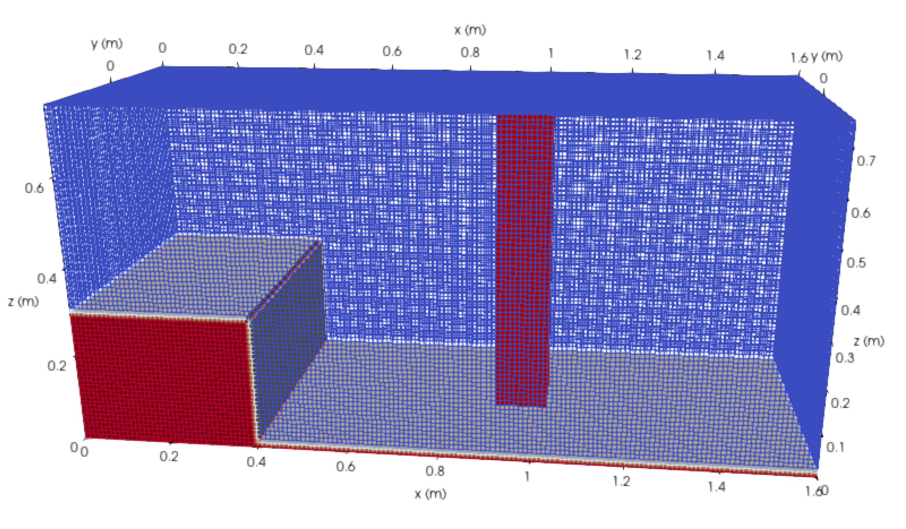
Figure 4 illustrates the setup of the numerical simulation. The dimensions of the tank are
. A volume of water with the size
is initially placed at the left end of the tank. The dimensions of the vertical obstacle are
. It is placed downstream of the volume of water with center of the bottom of the obstacle at
. As reported by Petroff and Yeh, the bottom of the tank was not completely drained in the physical experiment. Therefore, a thin layer of water with
in depth is setup in the present simulation as shown in
Figure 4.
It should be noted the way that the water is released in the present simulation is different from how the experiment was conducted. In the physical experiment, the water is blocked by a gate that is lifted vertically with finite speed at the beginning of the test, whereas in the simulation the water is released instantaneously. Lin and Chen [
25] discuss the influence of the opening speed of the gate on the time history of the impact force on the obstacle. Their results show that the peak of the impact force is delayed as the finite opening speed of the gate decreases.
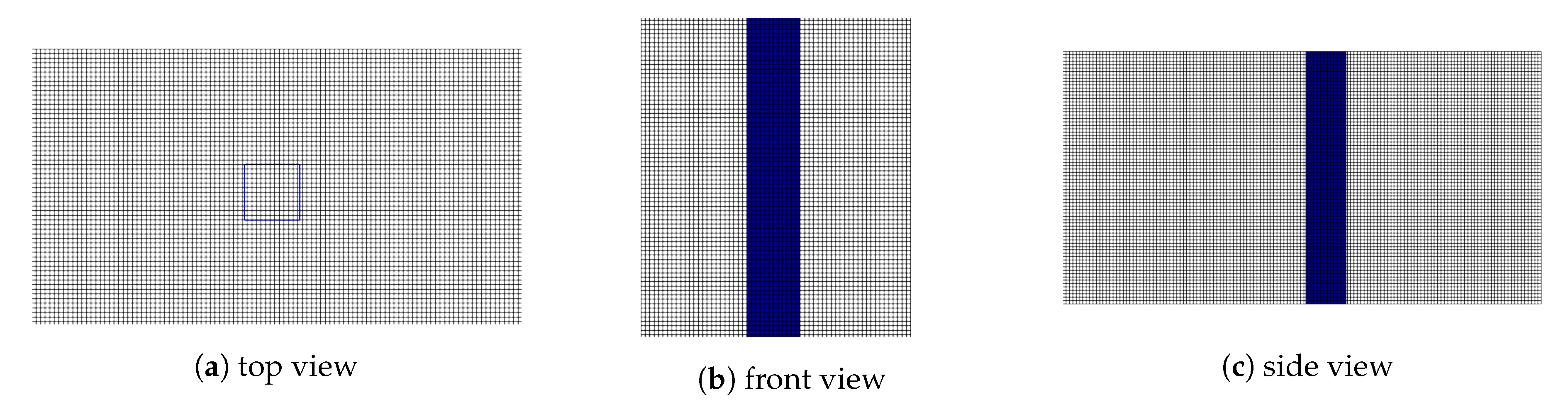
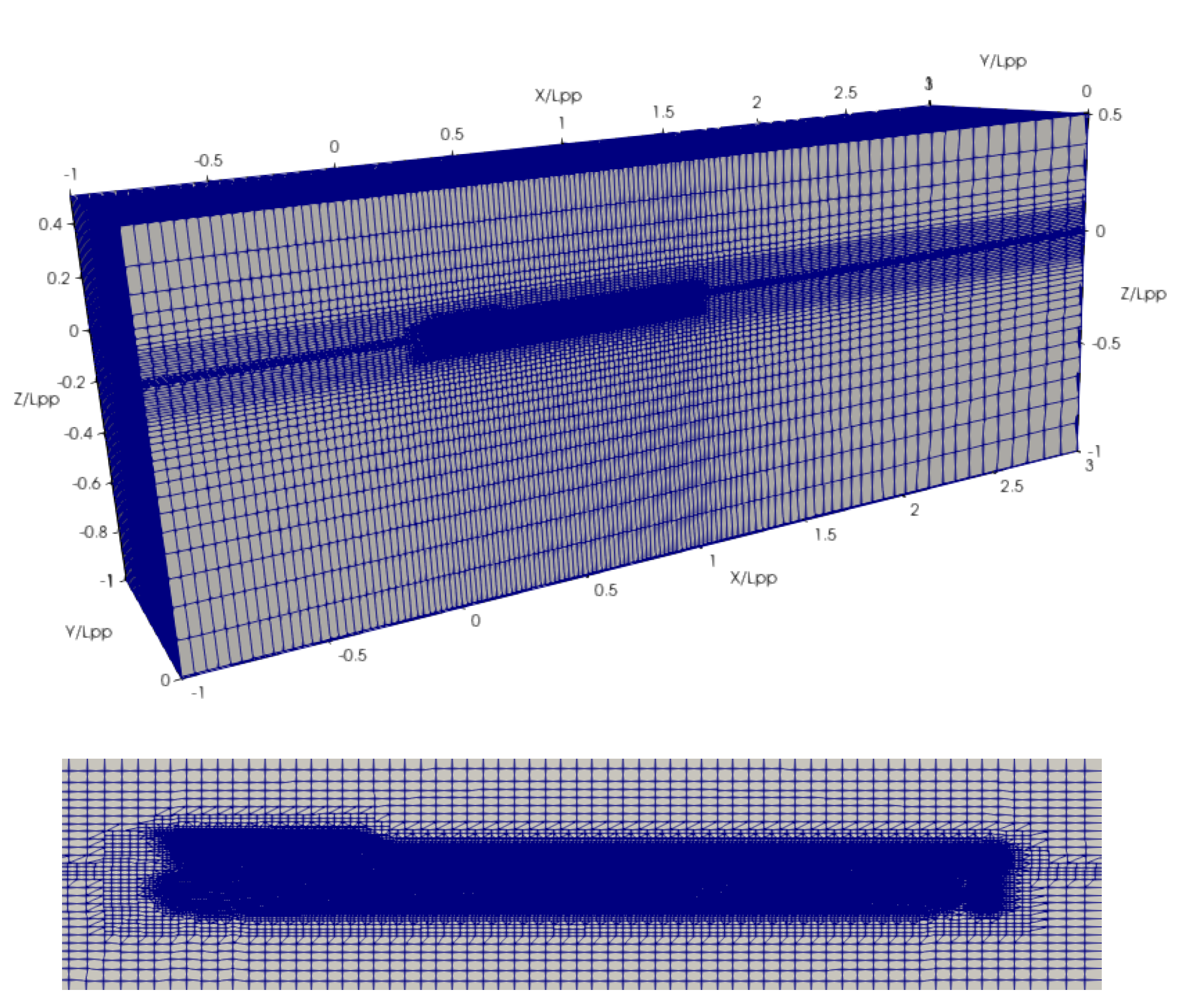
In the present simulations, the walls of the tank are represented by the body-fitted wall boundaries as shown in
Figure 4. The solid walls of the vertical obstacle are represented by an IB surface. A set of three background meshes with a refinement ratio of
in each direction is used to validate the solver. The total numbers of cells of the background meshes are
,
and
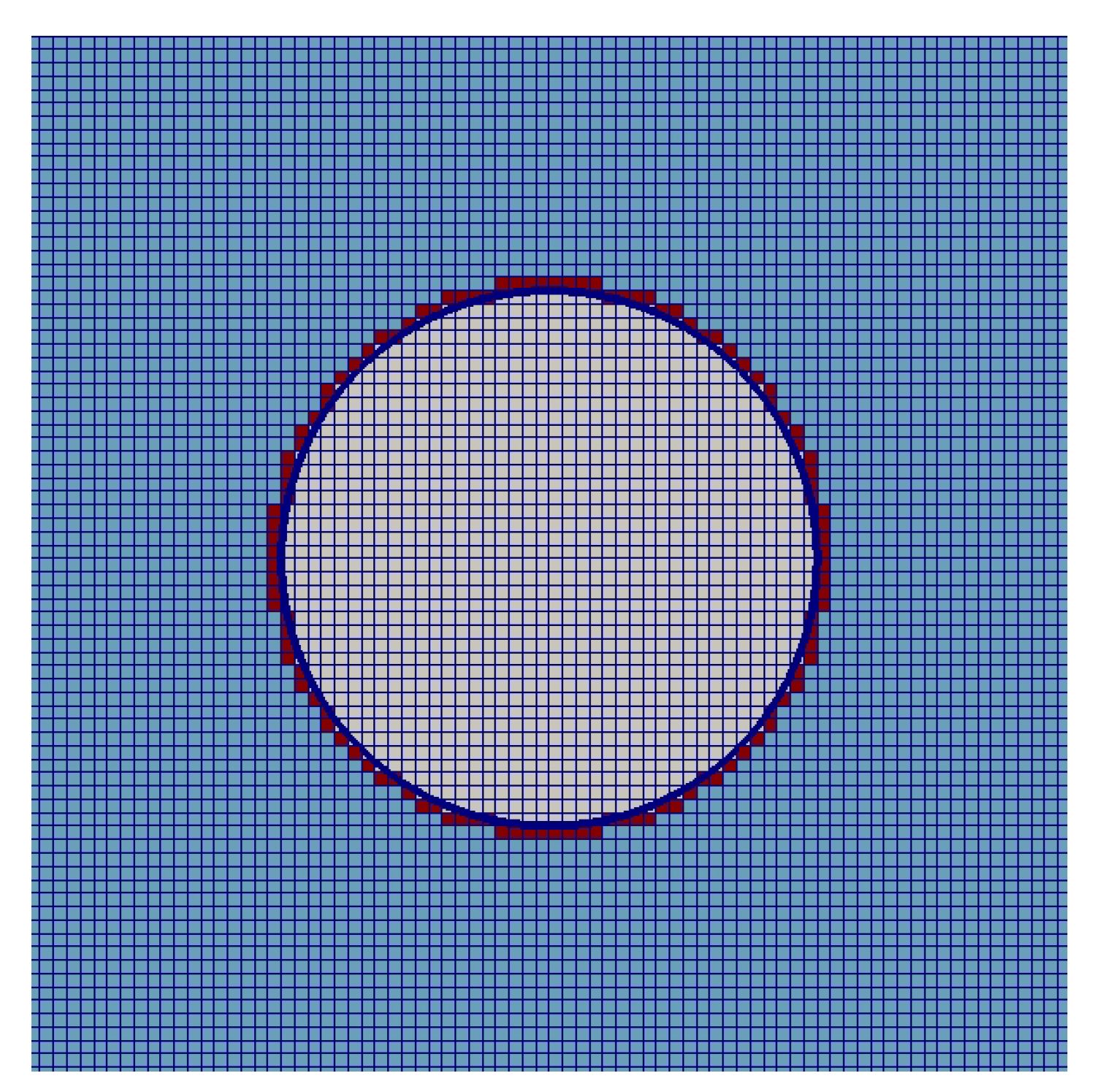
, respectively. The position of the IB in the tank is shown in
Figure 5.
The density and viscosity are , for the water, and , for the air. The gravitational acceleration is . In the simulations, the time step size is adjusted automatically to keep the Courant number less than 1.0.
A probe is used to record the flow velocity at a location in front of the obstacle at . In addition, the impact force on the obstacle is calculated.
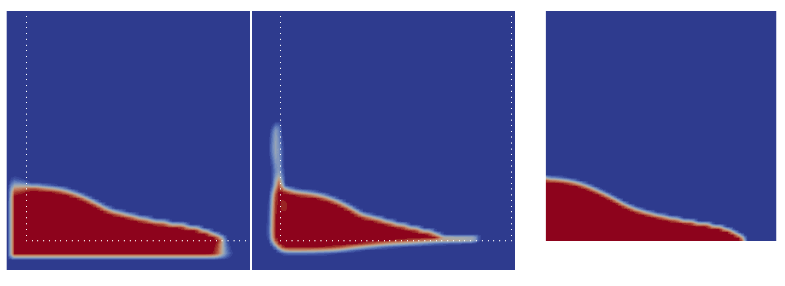
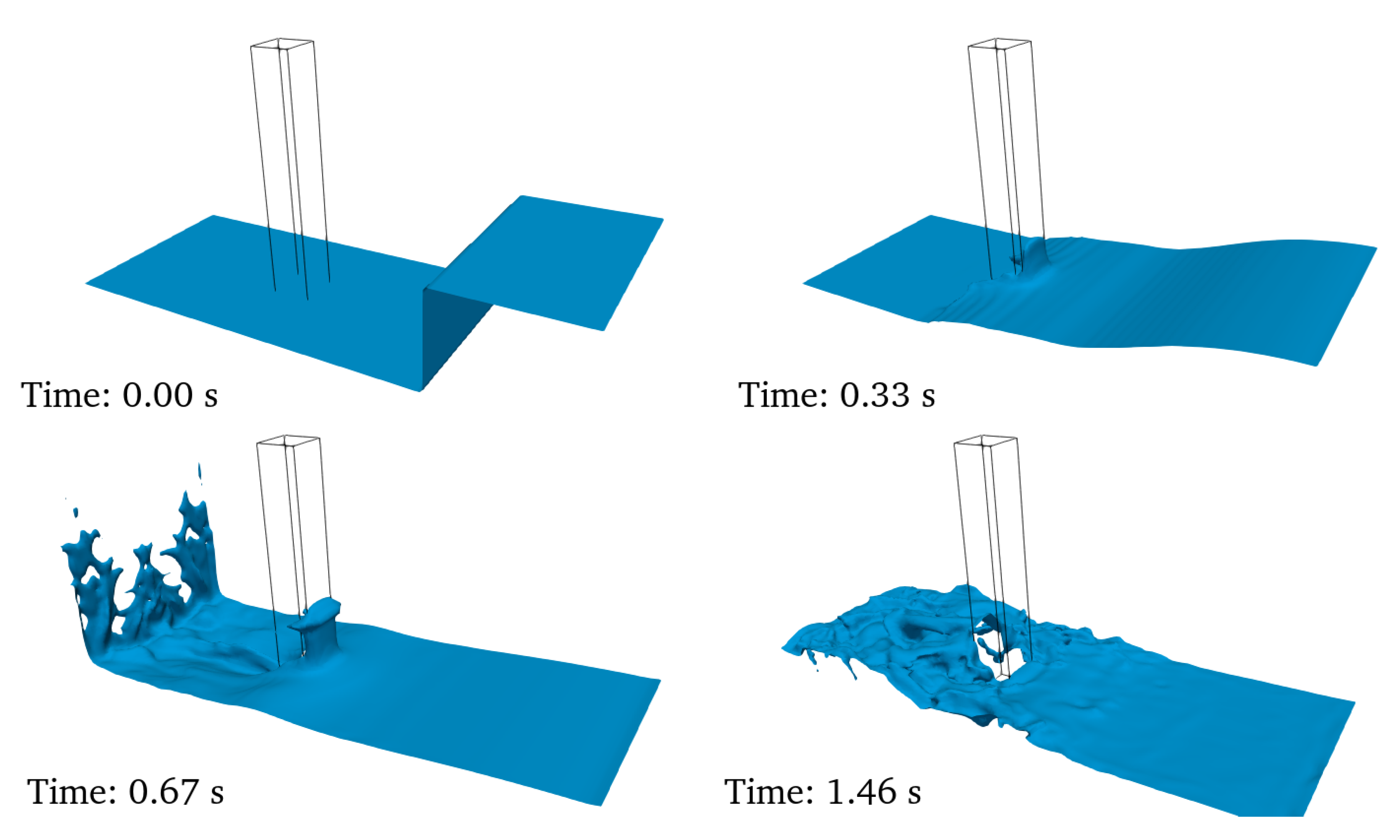
Figure 6 shows the wave propagation and its interaction with the obstacle at different time instants. It provides a general idea of what the critical phases of the dam-break problem look like. At
s, the water is released. After the water hits the front side of the obstacle, it runs up along the front wall and causes a large impact force. Afterwards, the water that travels around the obstacle joins together behind the obstacle, travels to the end of the tank, and hits the back side of the obstacle after being reflected by the end wall of the tank. It causes a second impact in the opposite direction compared to the first peak of impact. The second impact force is expected to be weaker than the first one because the velocity of the front of the wave is decreasing in general.
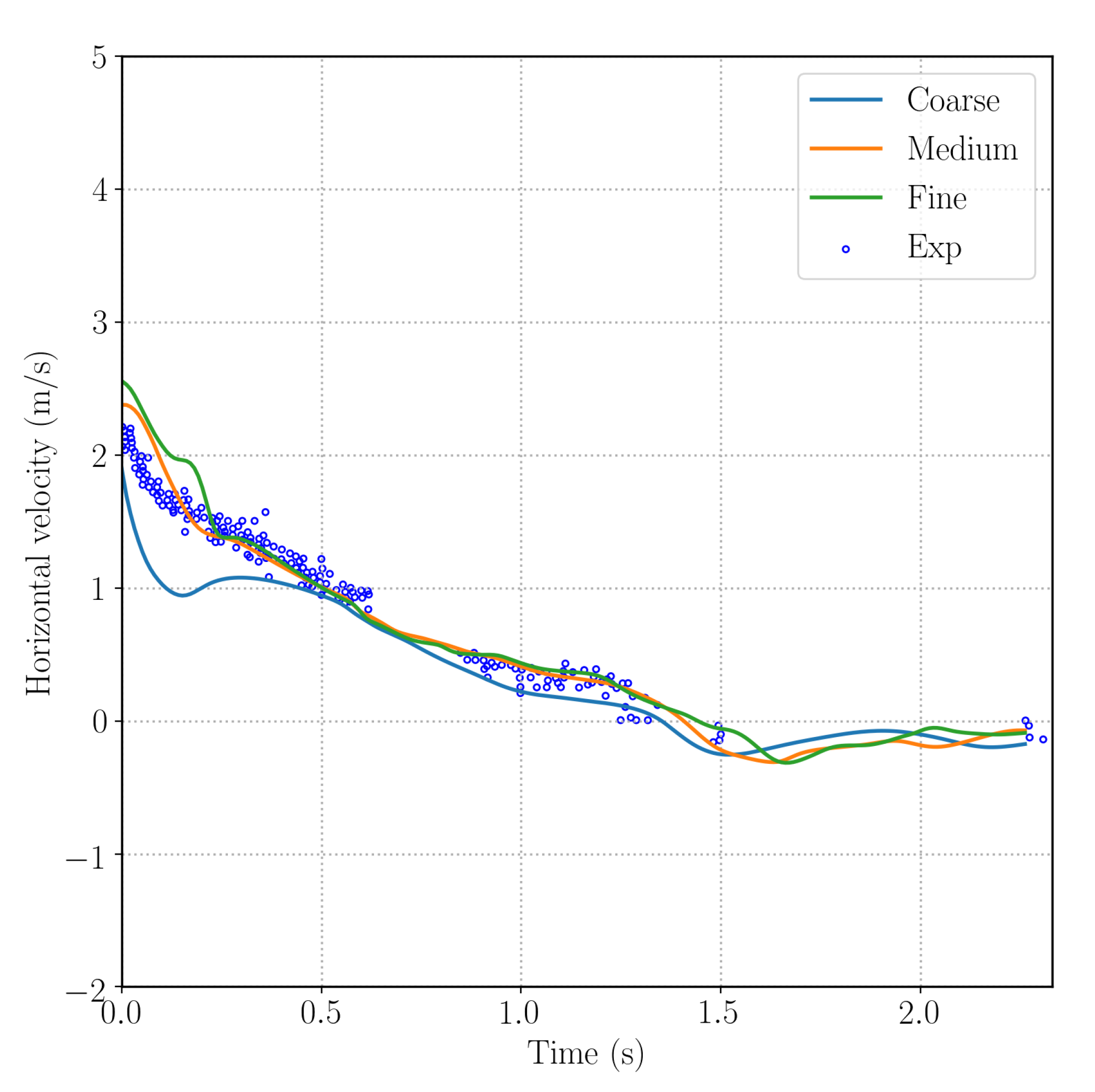
To further evaluate the accuracy of the solver,
Figure 7 shows the
x-component of the velocity at the velocity probe using all three background meshes. The data is shifted in time such that
s in the figure is the moment when the water first reaches the probe. Specifically,
in the figure corresponds to
s after the water is released. The experimental data is plotted together for the purpose of comparison. The gaps in the experimental data at
s and
s are due to the presence of bubbles in the water as explained in [
24]. The velocity at
is slightly overpredicted by the medium and fine meshes, which means the water moves faster in present simulations than in the experiment. It should be noted that in the simulations, the floor is set to be covered by a thin layer of water of thickness
. The layer of water is used to mimic the wet floor in the experiment. However it cannot perfectly reproduce the experimental environment. Another reason is that the gate in front of the water is released with finite speed in the experiment, which reduces the velocity at the water front near the floor. A similar conclusion is drawn in [
25] by investigating the influence of the release speed of the gate. The medium and fine meshes correctly predict the decrease in the velocity of the water (e.g.,
) due to the blockage of the obstacle. After
, the wave is reflected from the tank wall at
, and it is further blocked by the back side of the obstacle. The water near the bottom floor in front of the obstacle is almost stationary. This can be confirmed from
Figure 7 that the velocity at the probe drops to almost zero after
.
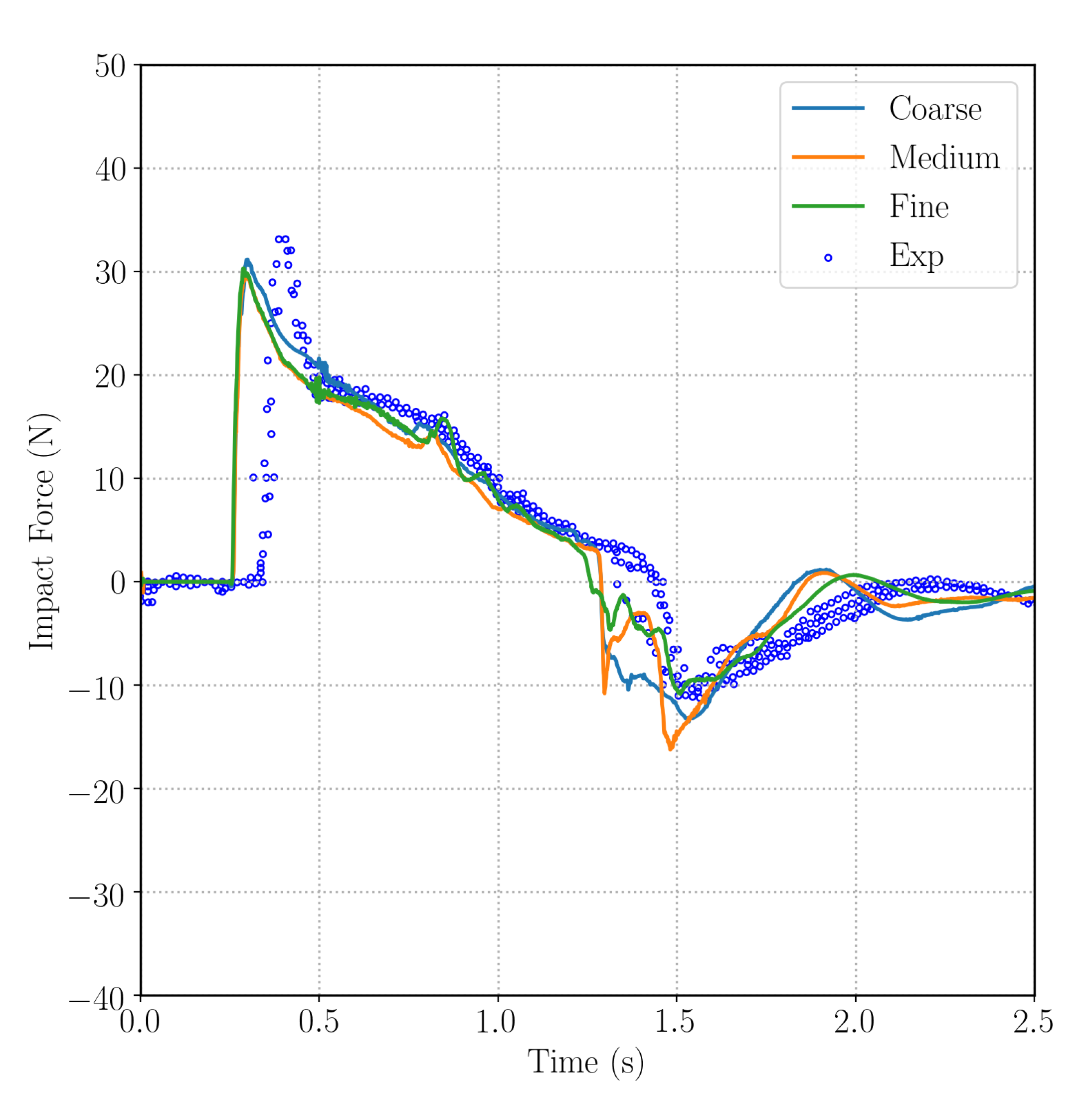
Figure 8 shows the impact force on the obstacle. It is worth pointing out that
in this figure corresponding to the time when the simulation starts, which explains the zero impact force at about
. The different background meshes predict a consistent start time of the impact. Compared with the experimental data, it can be seen that the first impact happens earlier than in the experiment, which is consistent to the behavior of the horizontal velocity at the velocity probe discussed before.
Figure 8 shows that the numerical results slightly underpredict the positive peak value at around
. Afterwards, the impact force decreases gradually to zero around
, which is consistent with experimental data. At
, the wave reflected from the end the tank arrives and impacts on the back side of the obstacle causing a negative peak of the impact force. During the last phase of the dam break, the impact force decreases to zero again.
In summary, the accuracy of the solver is demonstrated via the comparisons between the numerical solutions and the experimental data for the impact force and the horizontal velocity in the front of the obstacle.
3.1.2. Dam-Break No.2
In the previous section, the discussion is focused on the velocity of the water and the total impact force, which is an integrated variable. It is equally important to investigate the local pressure during the impact, as well as the water elevation at different places. To fulfill this goal, a different setup of the 3D dam-break problem with an obstacle is used in this section. The height of the obstacle is much smaller than in the previous case, which means the water also flows over the top of the obstacle. The physical experiment was carried out by the Maritime Research Institute Netherlands (MARIN, [
26]) to investigate the phenomenon of green water on the deck of a ship. Local pressure at different positions of the obstacle, and the water elevation at different locations of the tank were recorded in the experiment. The results of numerical simulations are also provided in [
26].
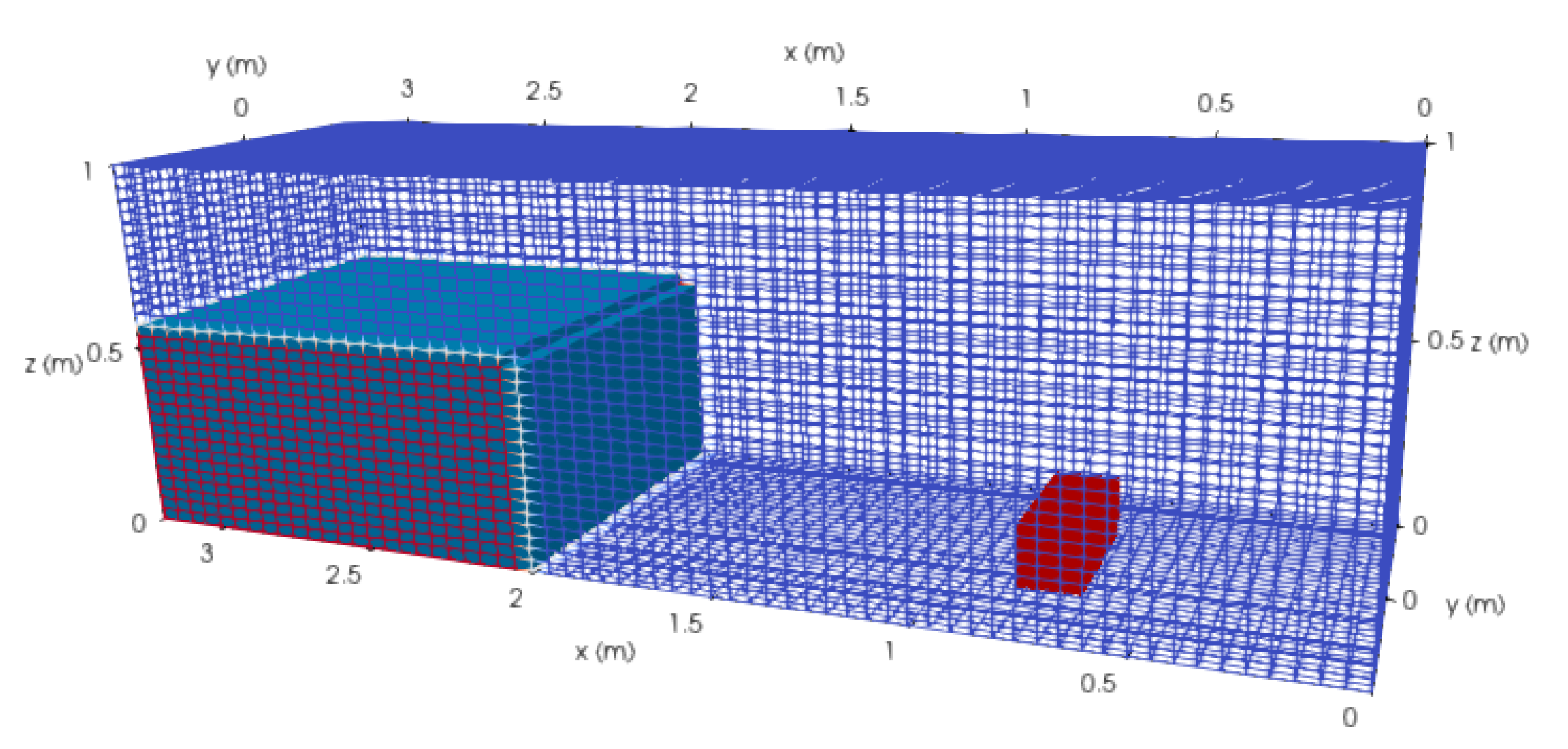
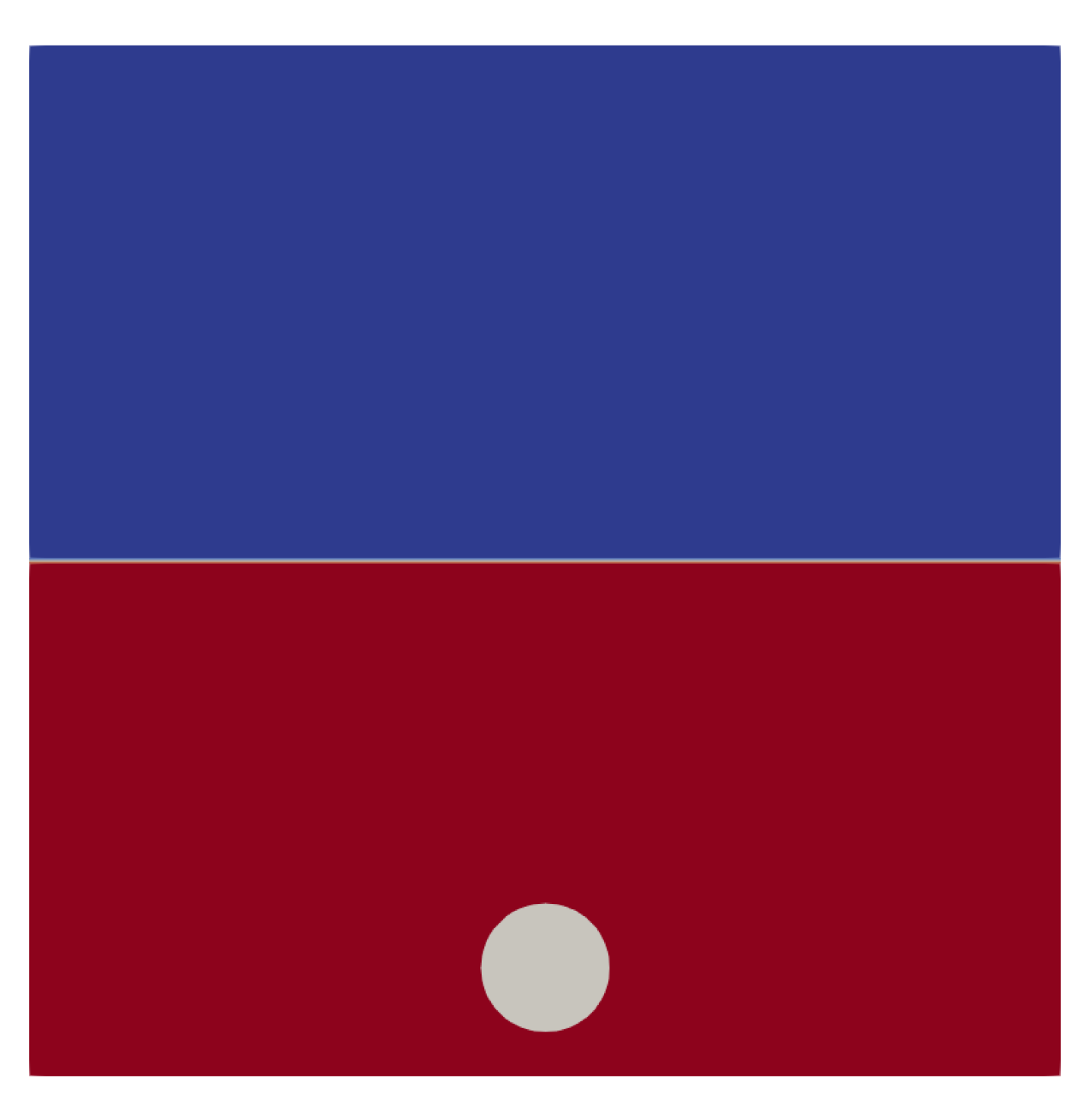
Figure 9 shows the computational domain and the numerical setup. The dimensions of the tank are
. At the beginning of the simulation, the volume of water with the size
is located at the end of the tank from
. A rectangular obstacle is placed in front of the dam to represent a container on the deck of the ship. The dimensions of the obstacle are
with its front side (the side which faces the dam) positioned at
. The water elevation is monitored at two places along the vertical plane
, which are
and
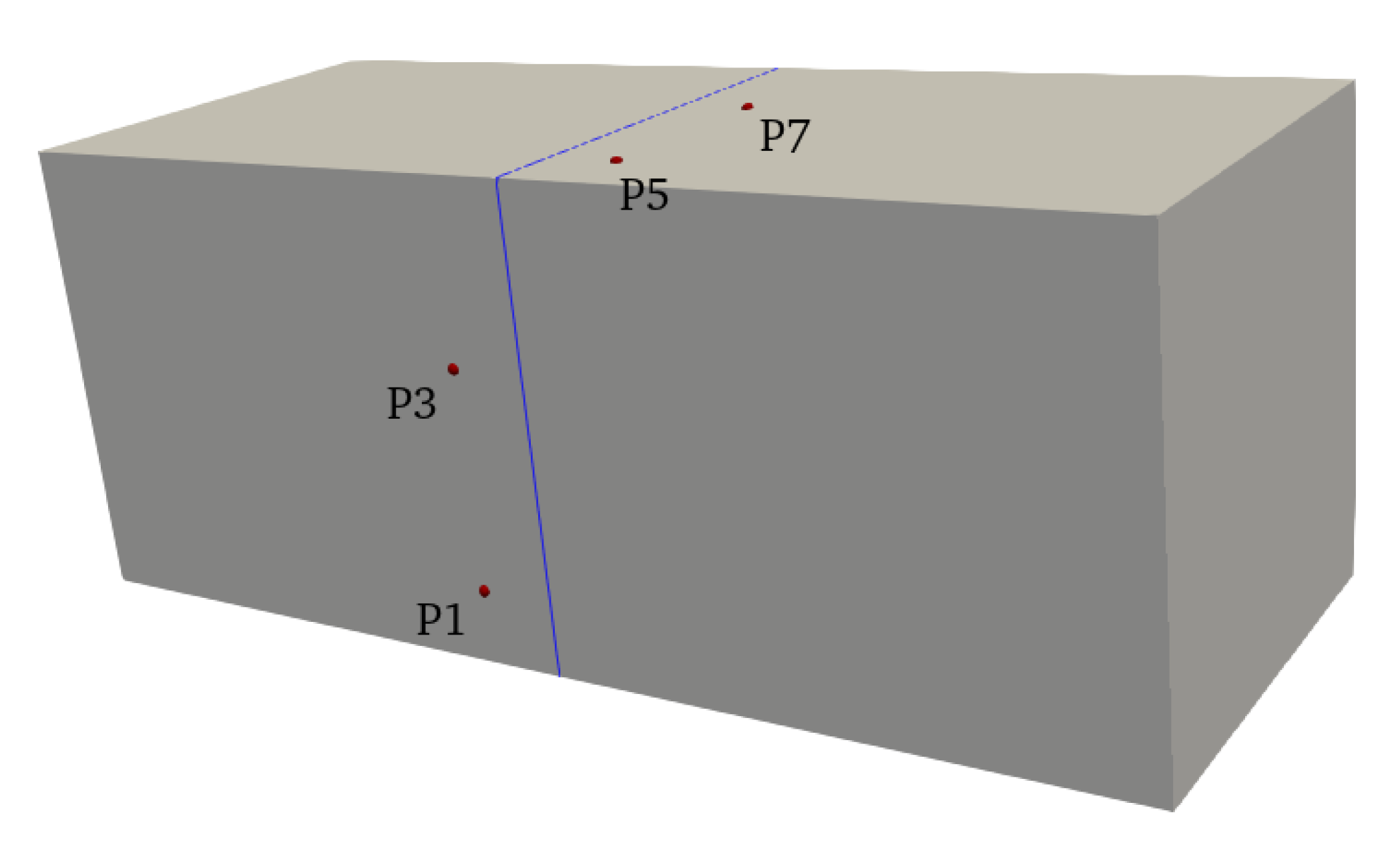
. Eight sensors are used to record the local pressure on the top and front sides of the obstacle, and the locations are listed in
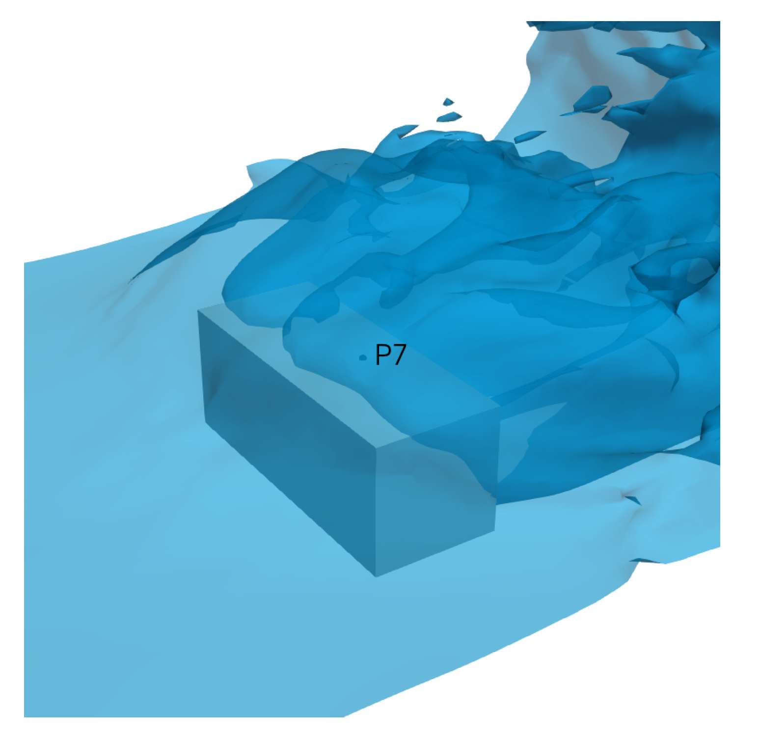
Table 1. The numerical results of the time histories at the pressure sensors P1, P3, P5 and P7 are compared with the experimental data. The locations of these four sensors are illustrated in
Figure 10. The sensors P1 and P3 are on the side facing to the initial volume of water. The blue solid line represents the plane
as a reference.
The density and viscosity of the water are , , and , for the air. The gravitational acceleration is . Similar to the previous section, a set of three background meshes with a refinement ratio of in each direction is used. The number of cells of the background meshes are , and , respectively. All the sides of the tank are represented by the body-fitted boundary conditions as no-slip walls, and the obstacle is modeled with an IB. The time step size is adjusted automatically to keep the global Courant number less than 0.75 and the Courant number near the free surface less than 0.3.
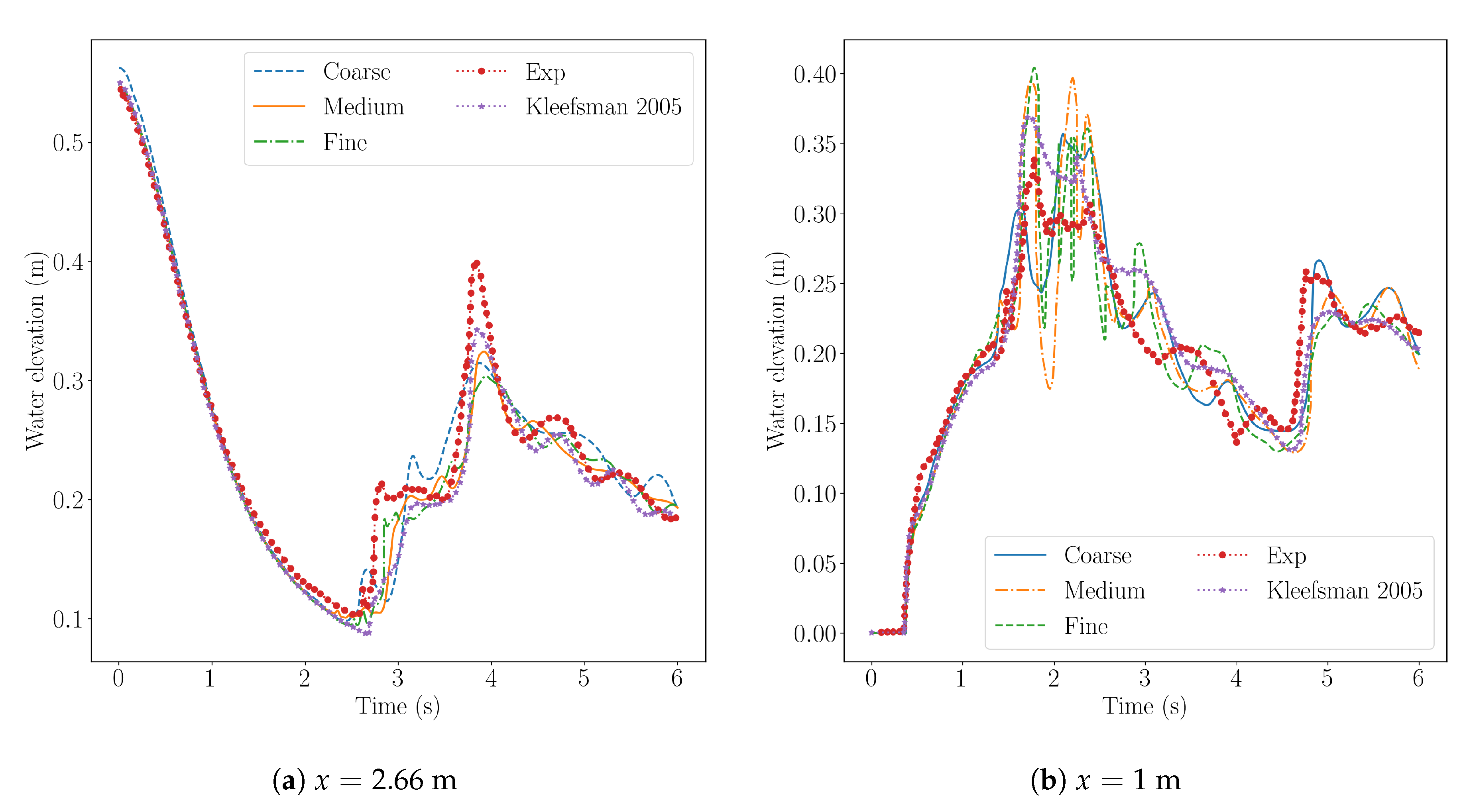
Figure 11 shows the time histories of the water elevation at the locations
and
, which are inside the initial position of the dam and in front of the obstacle, respectively. During the initial part of the time series the comparison between the experiment and simulation is very close. At about
and
, the water reflected from the wall of the tank at
arrives to the two probes, and causes a random unsteady and high frequency response. For the second part of the time histories, there are differences between the numerical results and the experimental data with regard to the high frequency part, yet the mean elevation is in very close agreement. For example in the probe at
, the front of the water arrives at around
s, and the numerical results accurately capture the instant when the air–water interface starts to rise in accordance with the experiments.
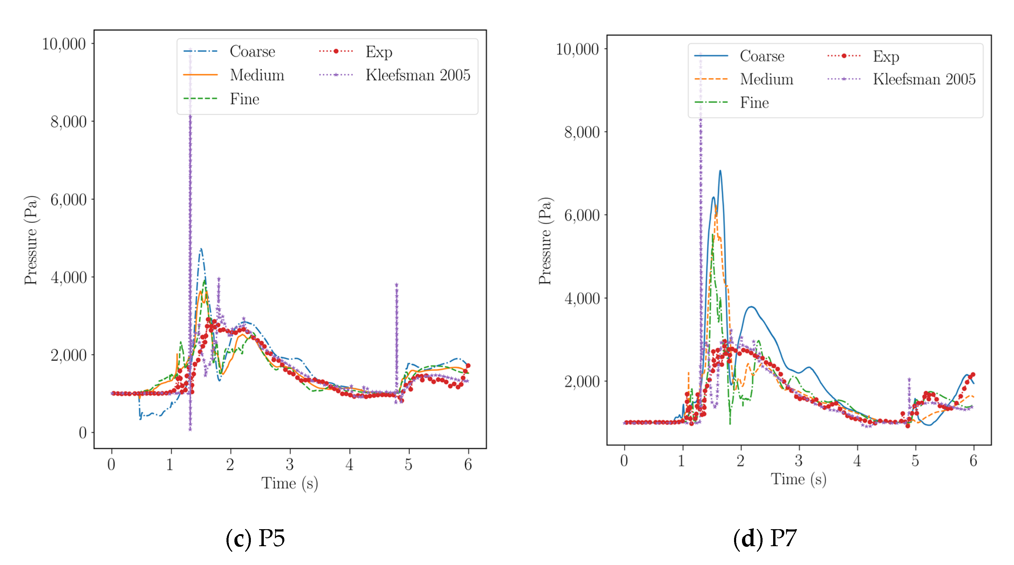
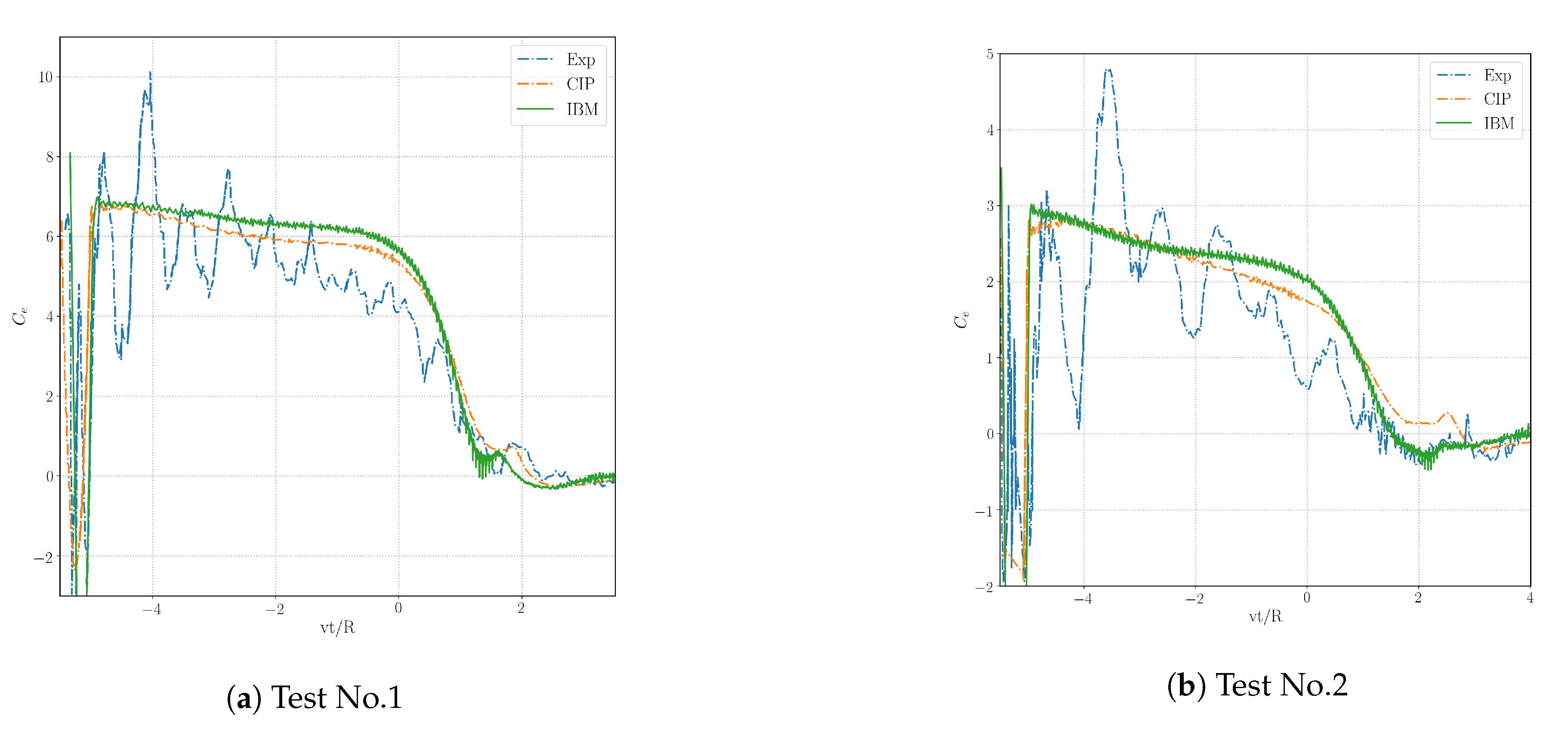
As shown in Figure
12, the time histories of the local pressure at four different sensors are selected to compare with the experimental data. The present numerical simulation captures the behavior when the water first impacts the sensors, especially for the ones on the front side of obstacle. The peak pressure at P1 matches with the experimental data very well, while the peak pressure at P3 is underpredicted by the fine mesh. At around
, the pressure at both sensors drops gradually.
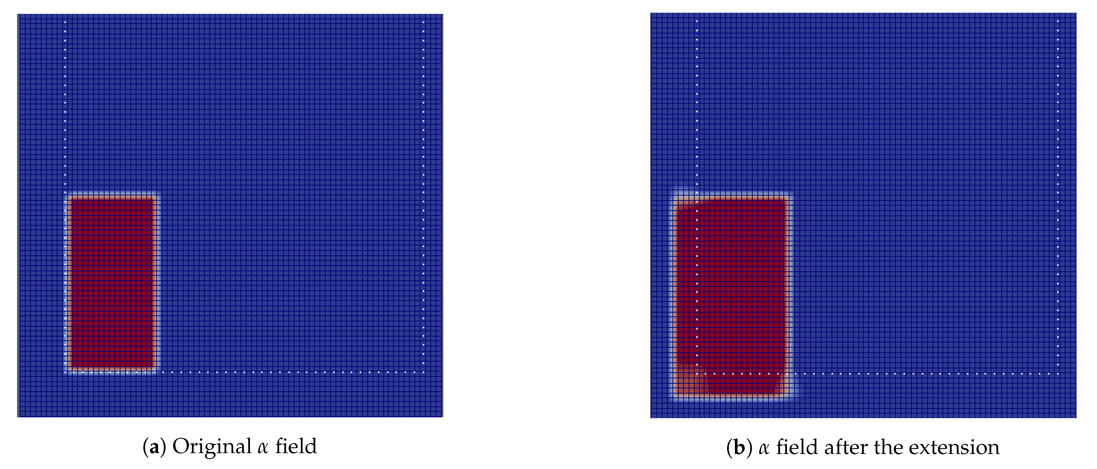
For the numerical results at P5 and P7, which are on the top surface of the obstacle, the numerical results show a large oscillation. It is because when the water flow over the obstacle, the large vertical velocity of the water causes the water to detach from the surface of the obstacle. Subsequently, air is entrapped when the water starts to impact on the top the obstacle. However, the effect of air compressibility is not considered in the current solver.
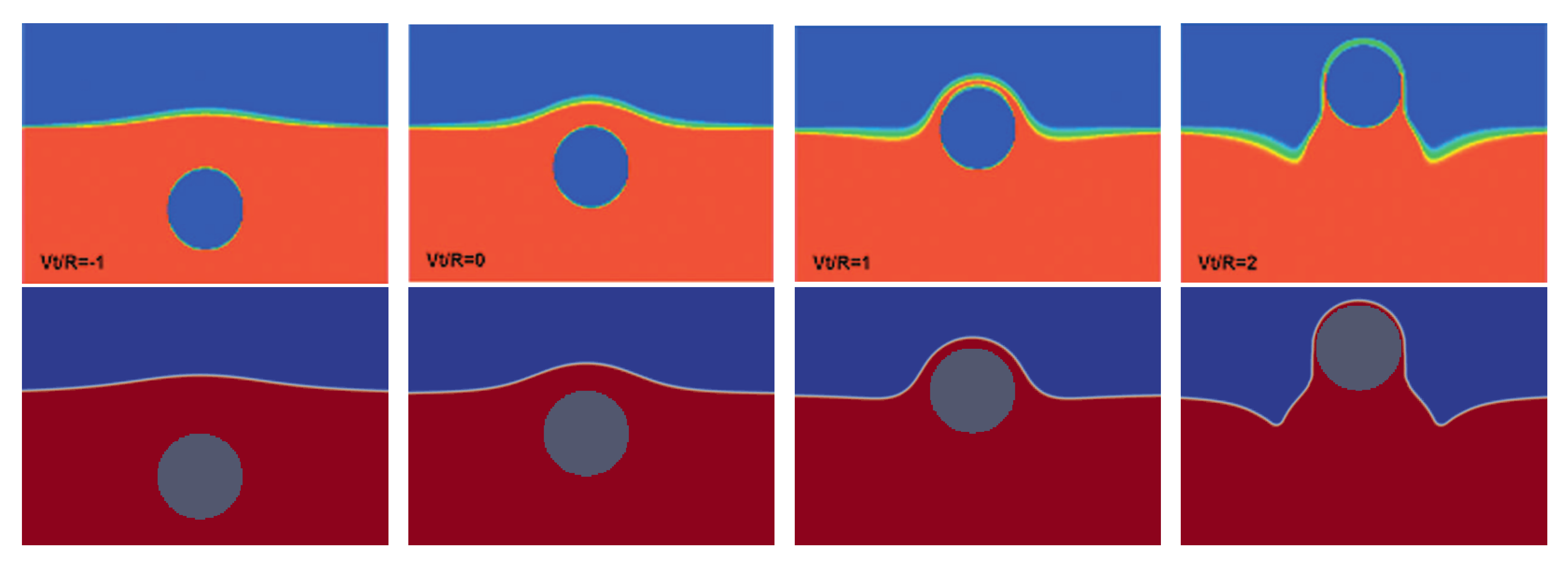
Figure 13 shows the profile of the air–water interface around the pressure sensor P7 at around
. It can be clearly seen that the air is entrapped and a bubble is formed around P7. As a result, the large oscillation appears in the numerical results at P5 and P7 in the limitations of the current numerical framework.
Overall, the results demonstrate that the present IBM solver can handle the problems of wave interaction with solid walls with respect to the evolution of the air–water interface, velocity of the water, force on the obstacle and the local pressure due to the impact.


