Impact of Hard Fouling on the Ship Performance of Different Ship Forms


Abstract
1. Introduction
2. Materials and Methods
2.1. Governing Equations
2.2. Resistance, Open Water and Propulsion Characteristics
3. Computational Model
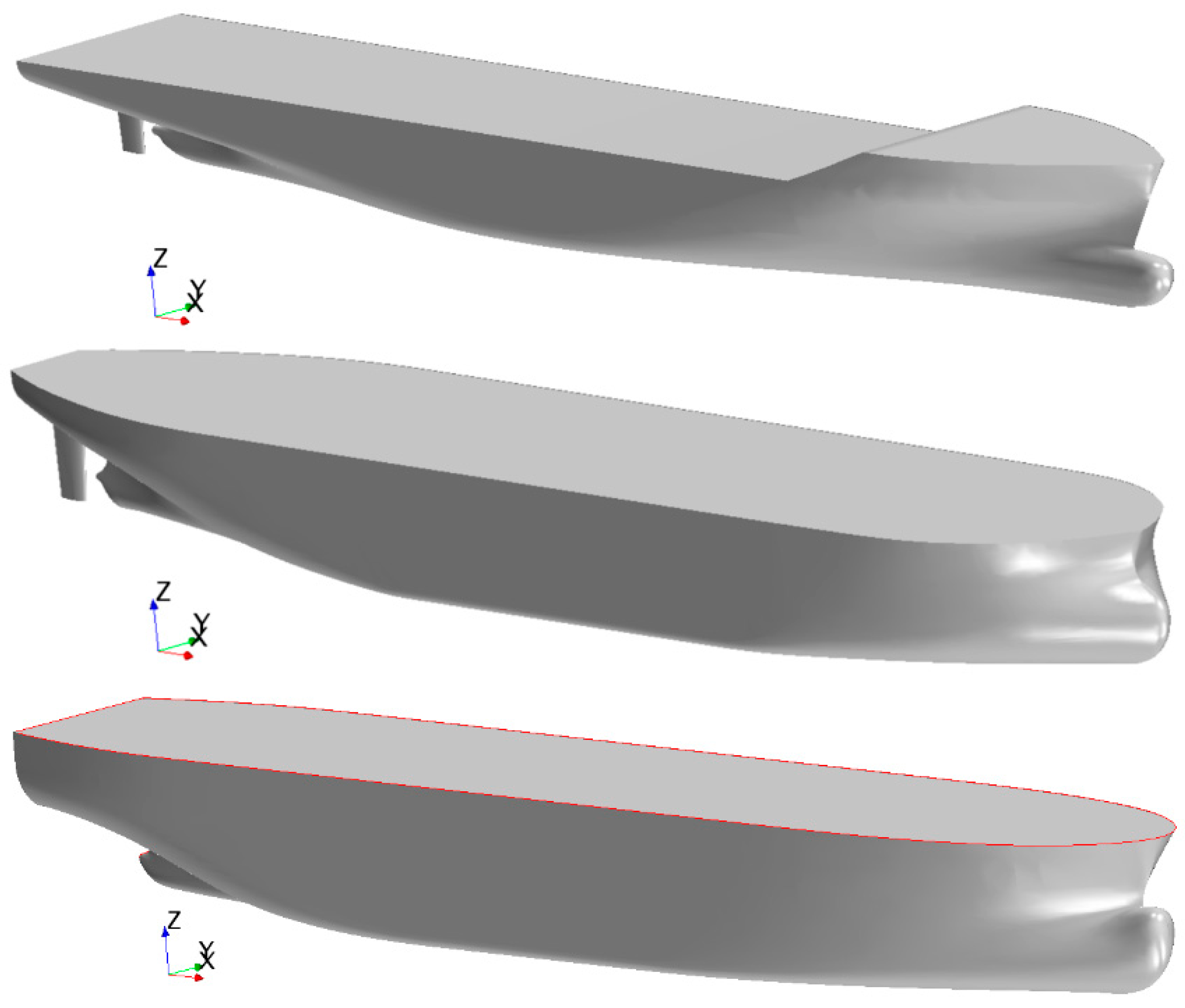
3.1. Case Study
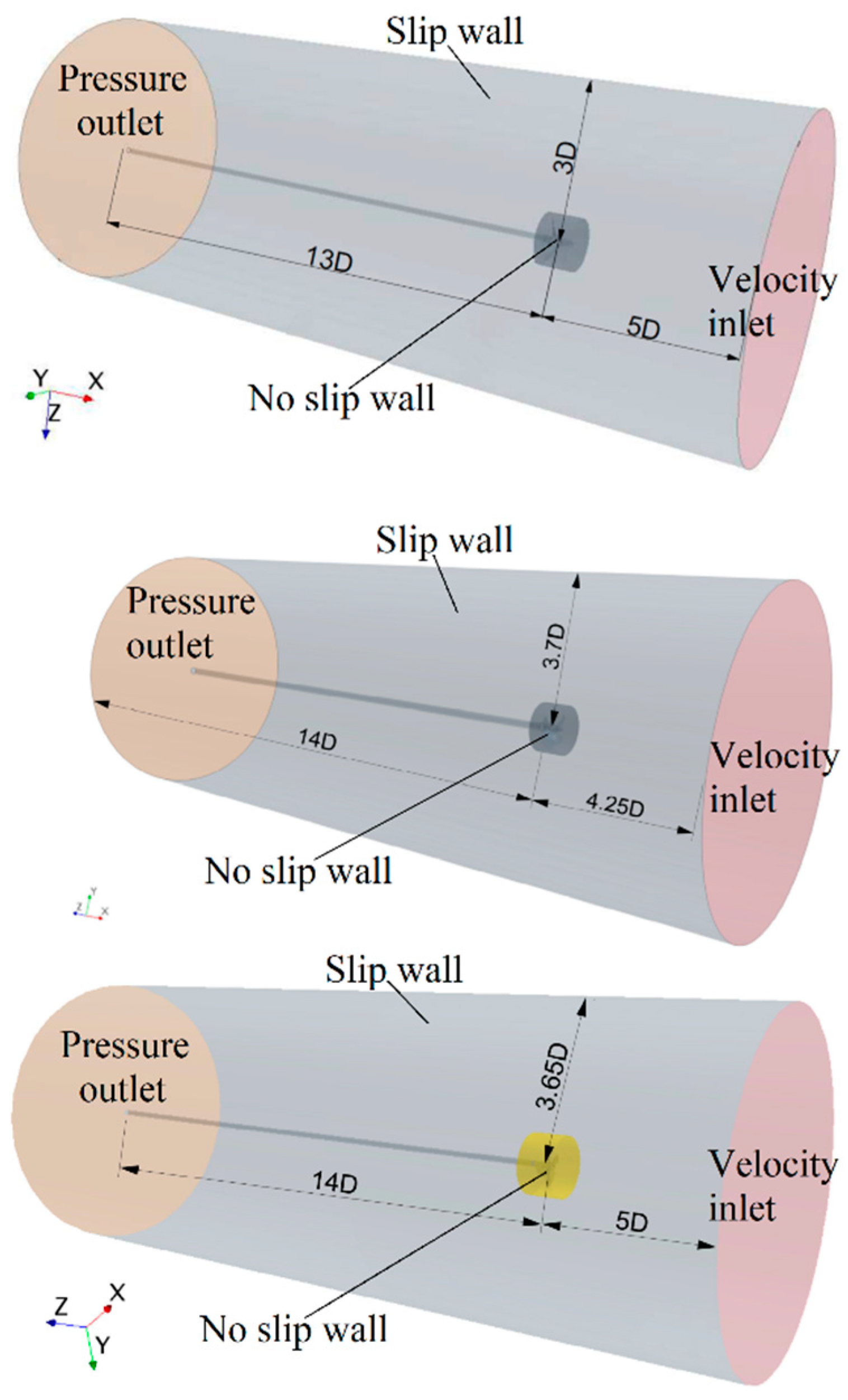
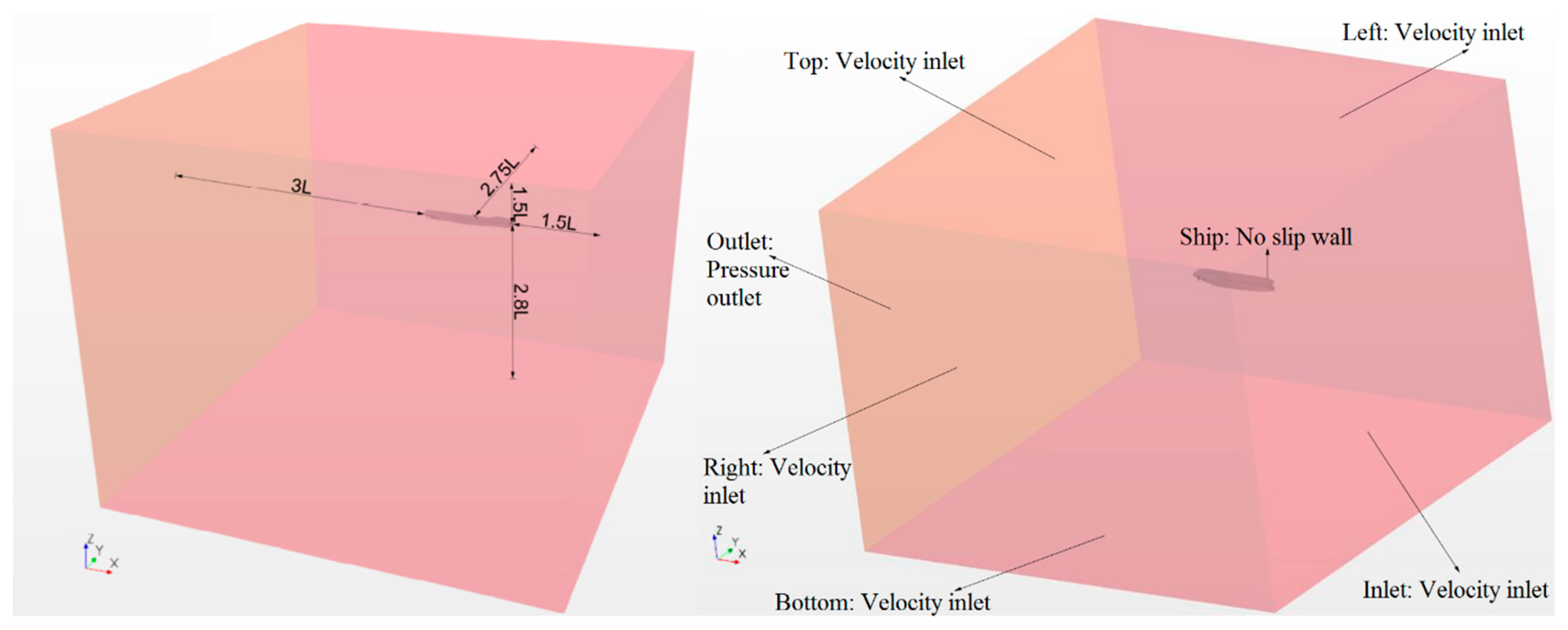
3.2. Computational Domain and Boundary Conditions
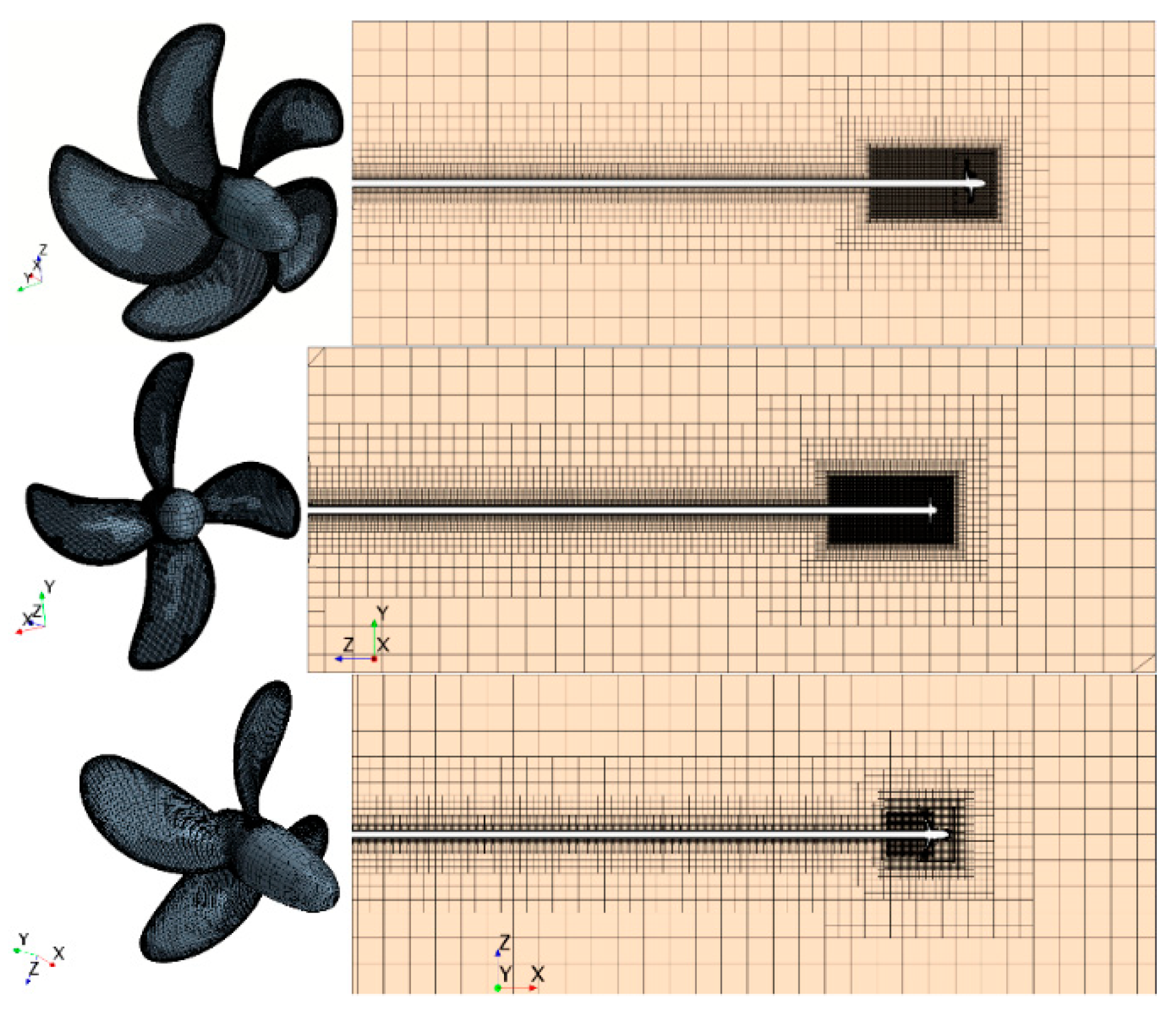
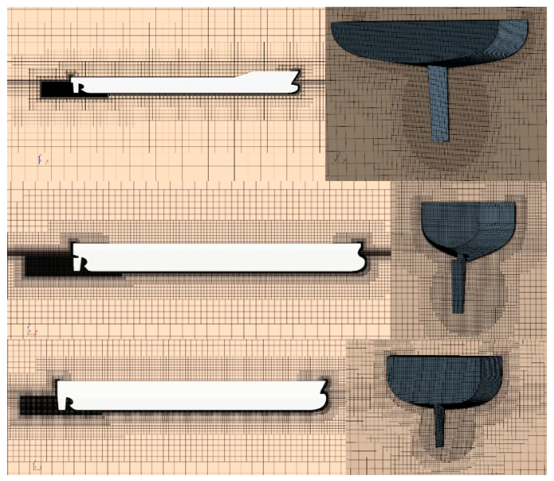
3.3. Discretization of Computational Domain and Computational Setup
4. Verification and Validation Study
4.1. Verification Study
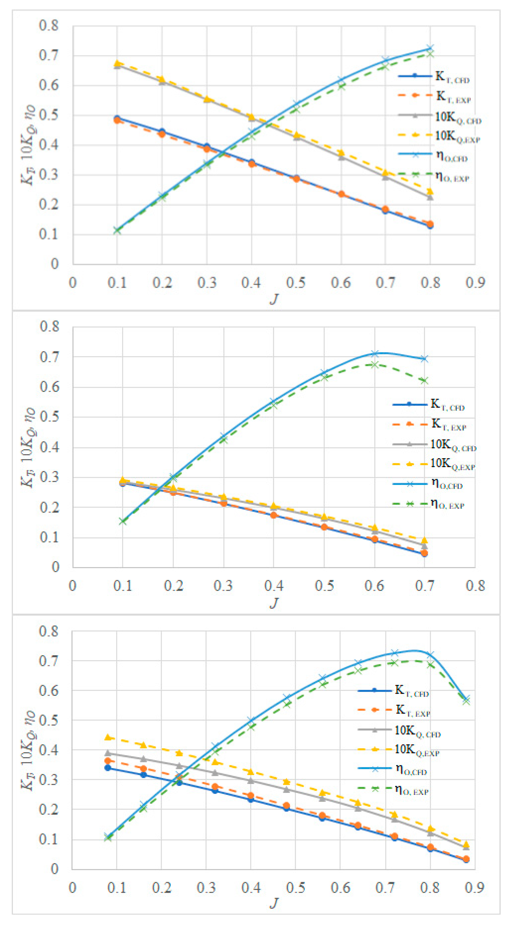
4.2. Validation Study
5. The Impact of Hard Fouling on the Ship Performance
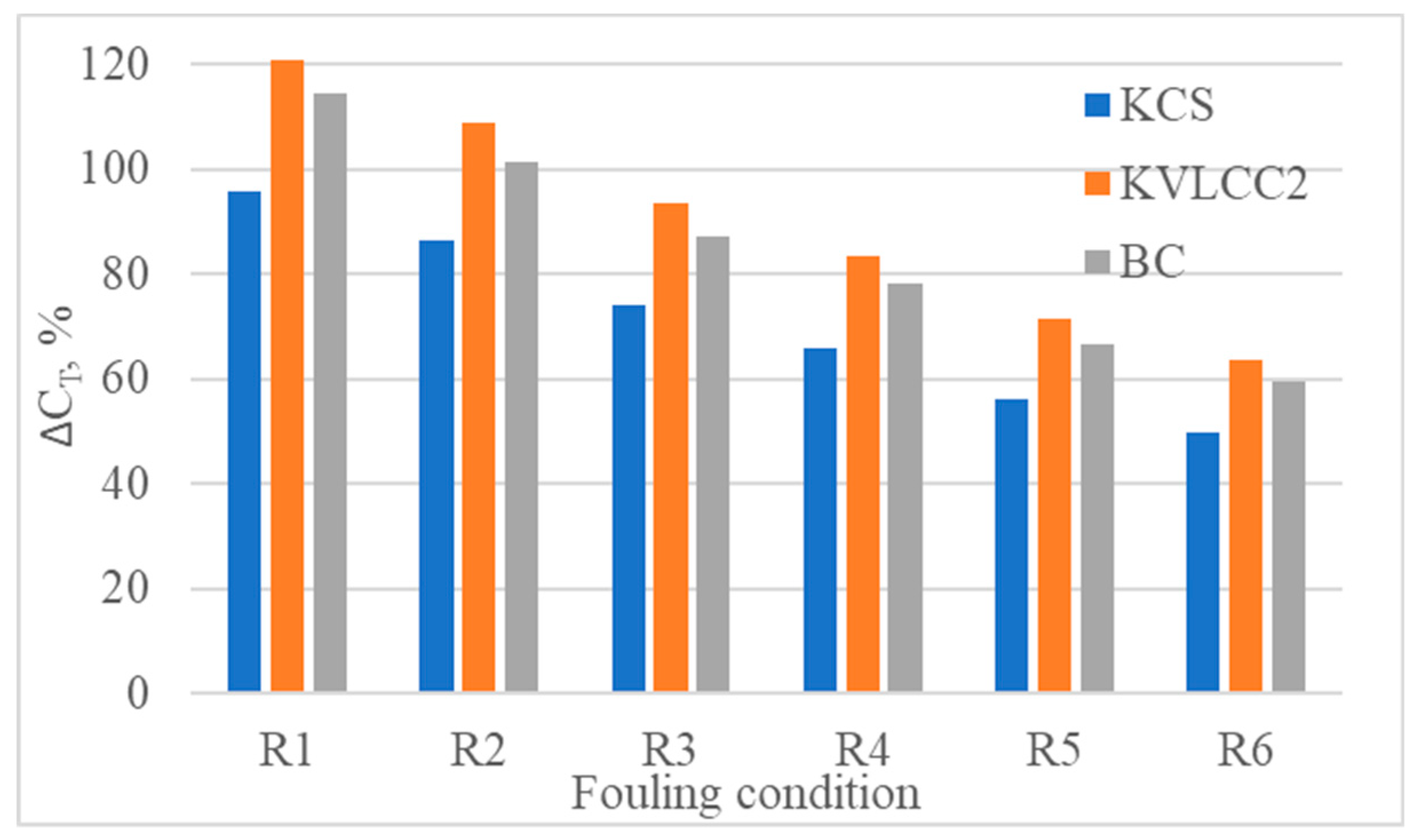
5.1. The Impact of Hard Fouling on Resistance Characteristics
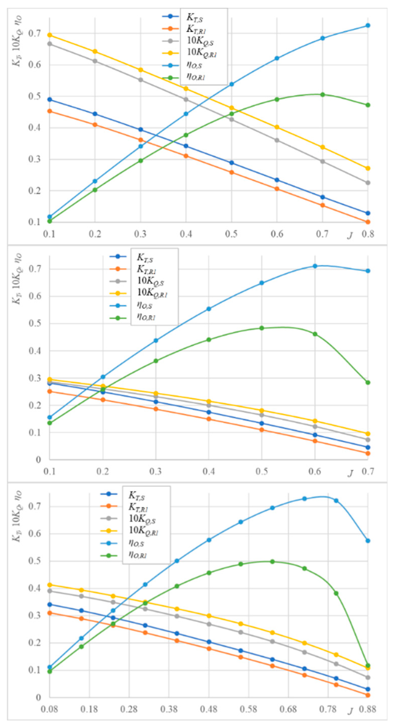
5.2. The Impact of Hard Fouling on Open Water Characteristics
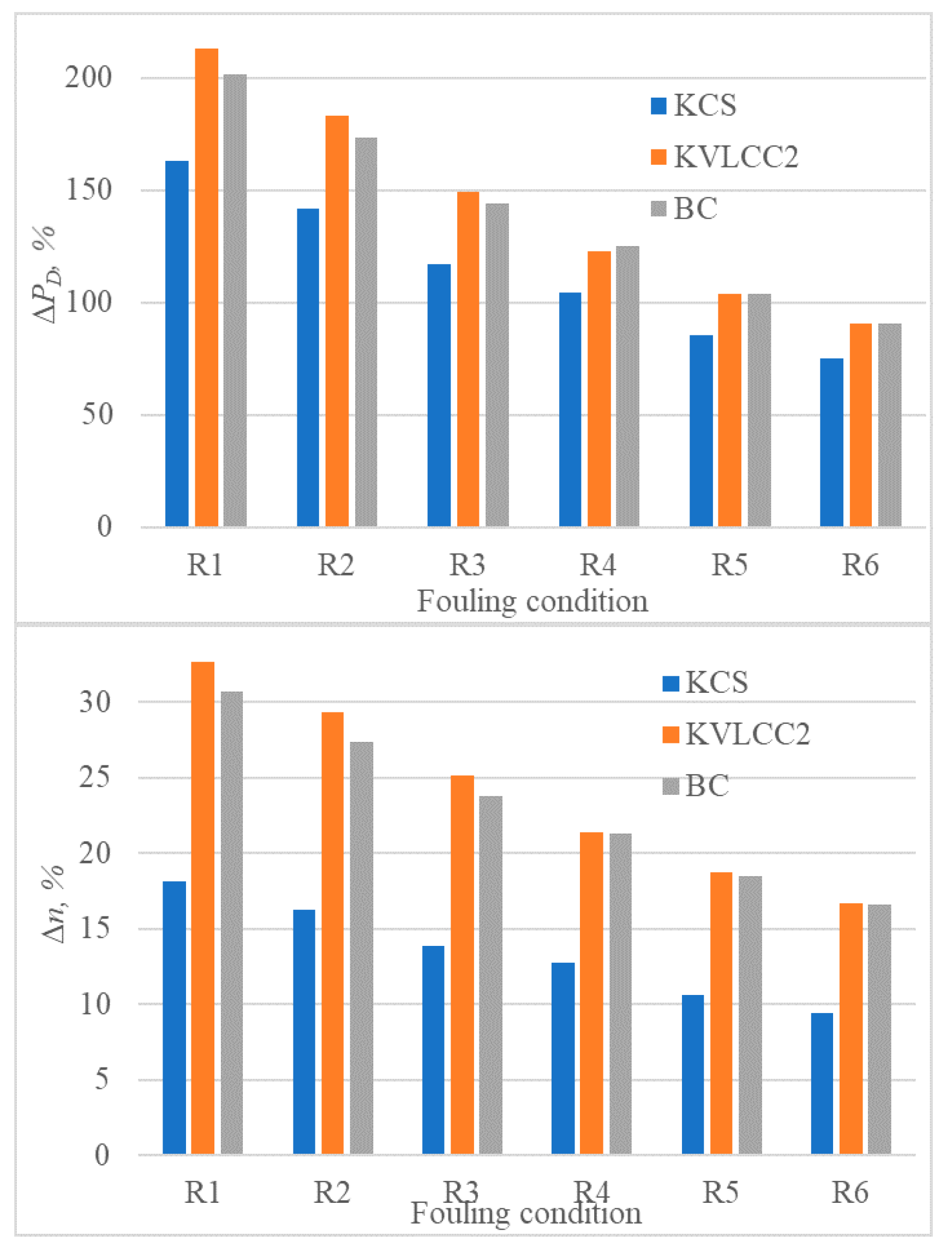
5.3. The Impact of Hard Fouling on Propulsion Characteristics
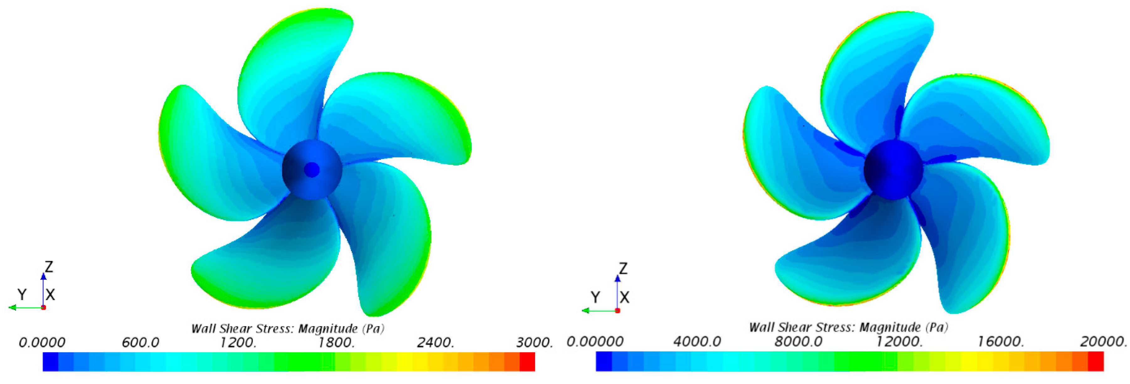
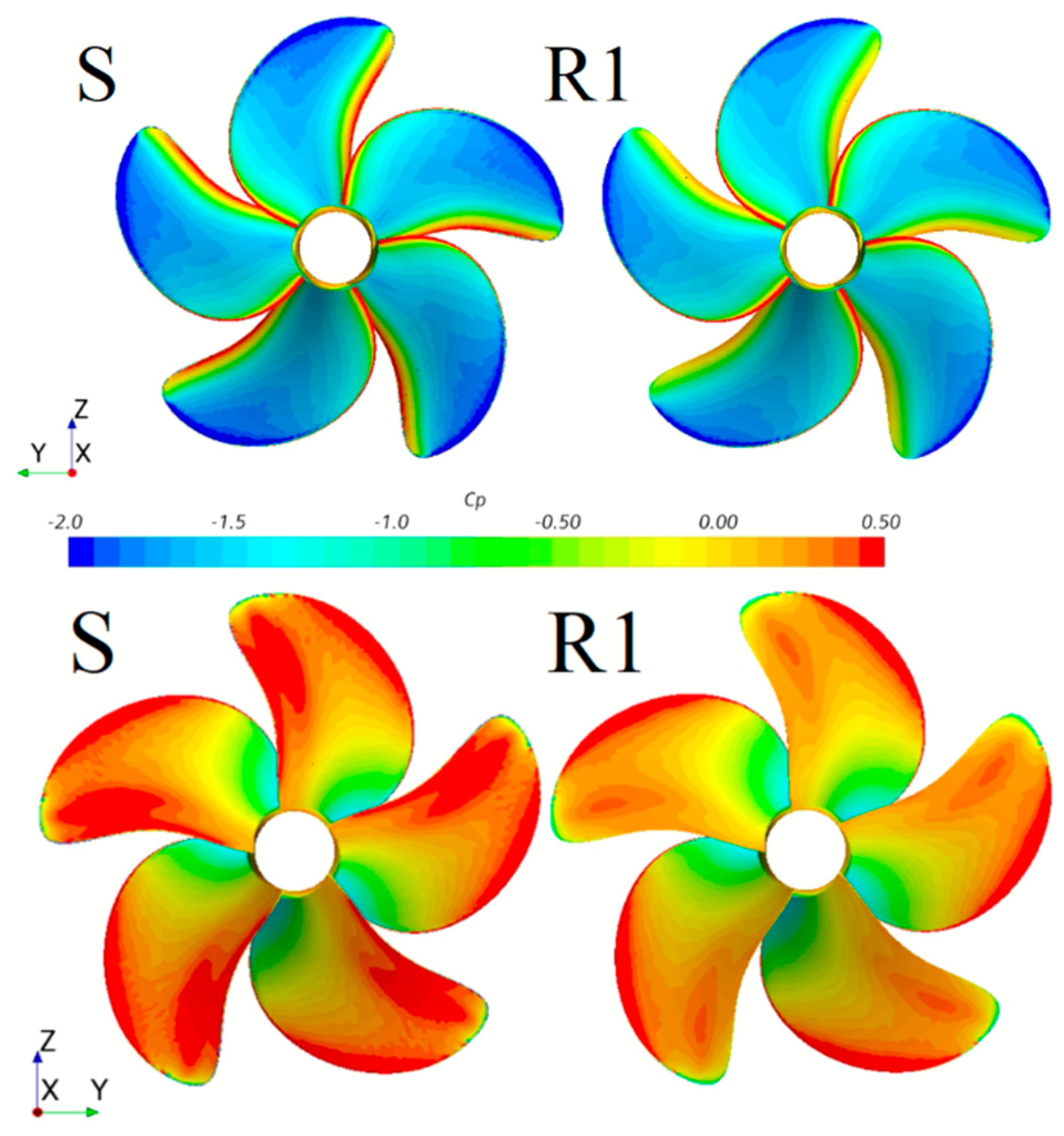
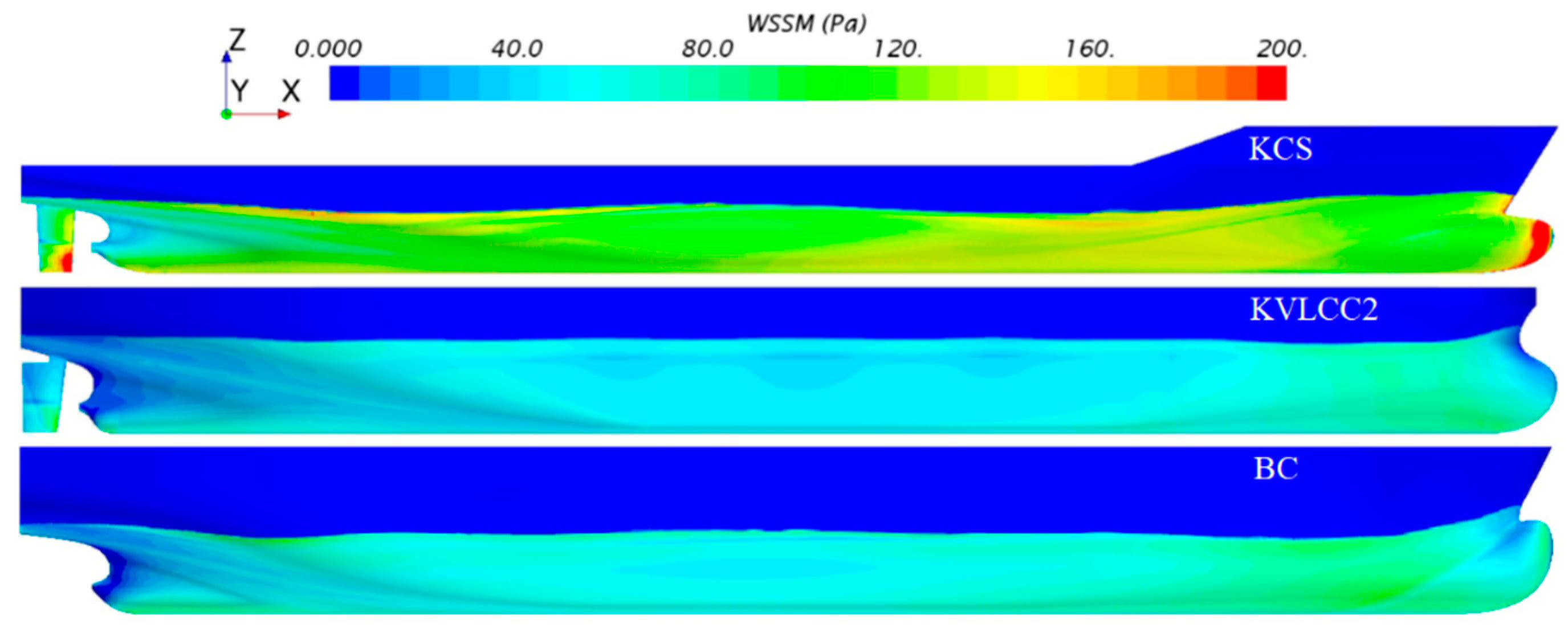
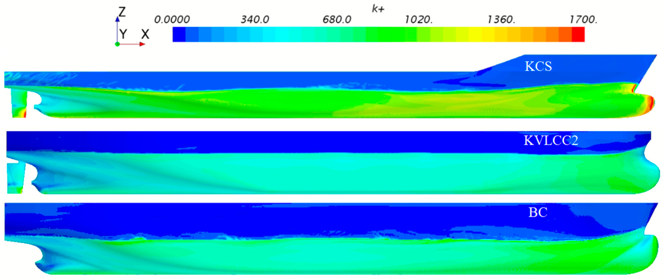
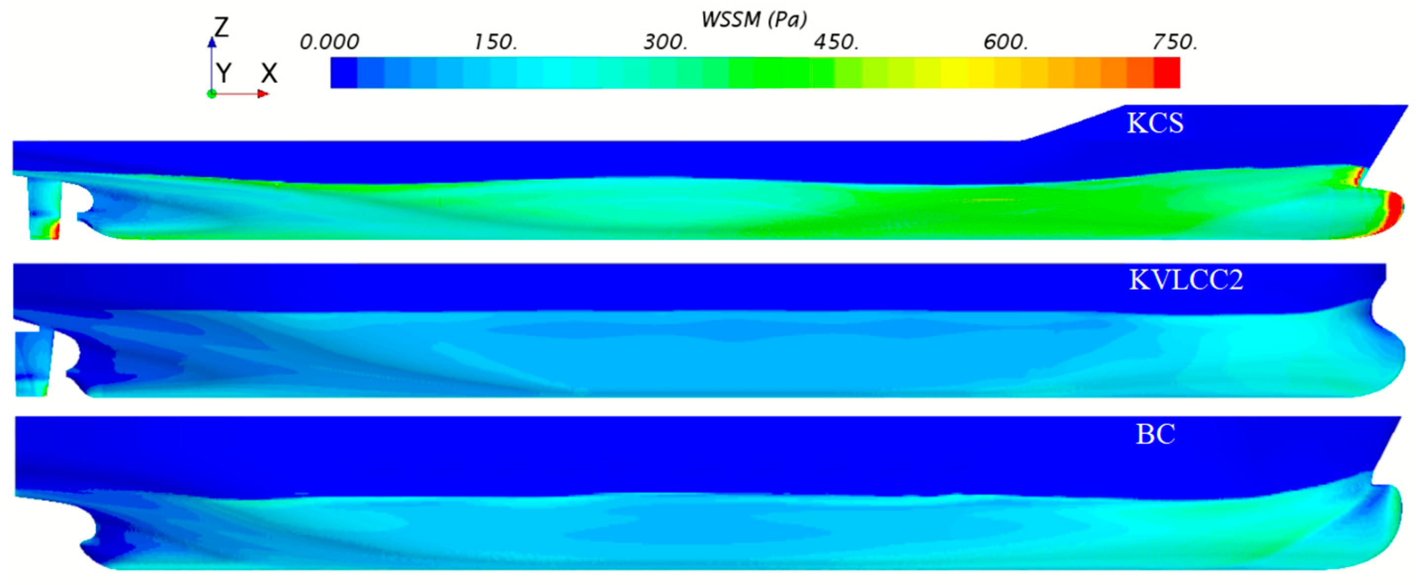
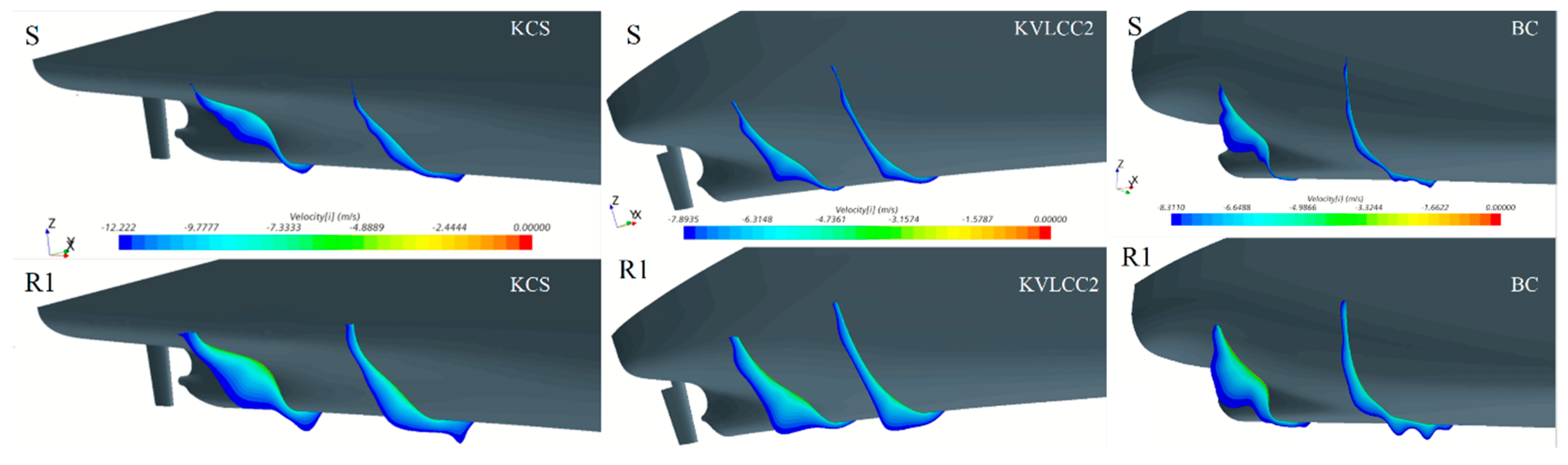
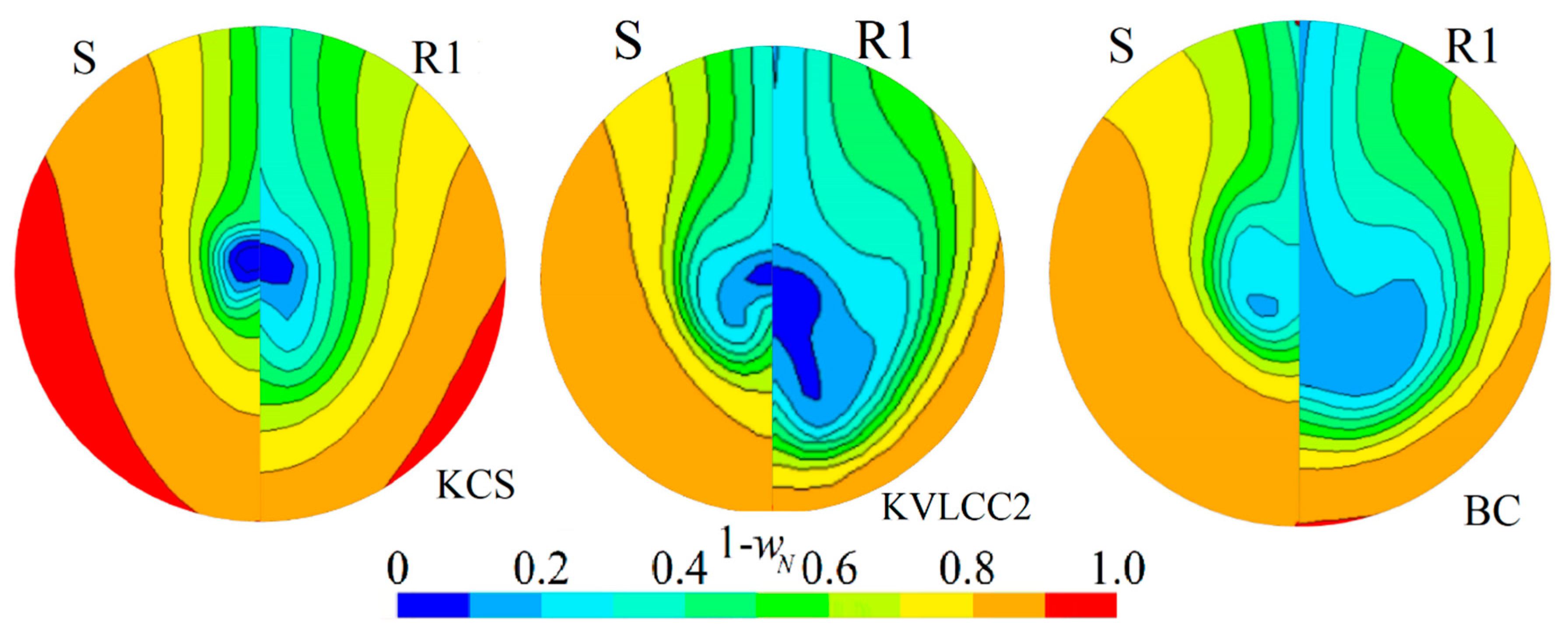
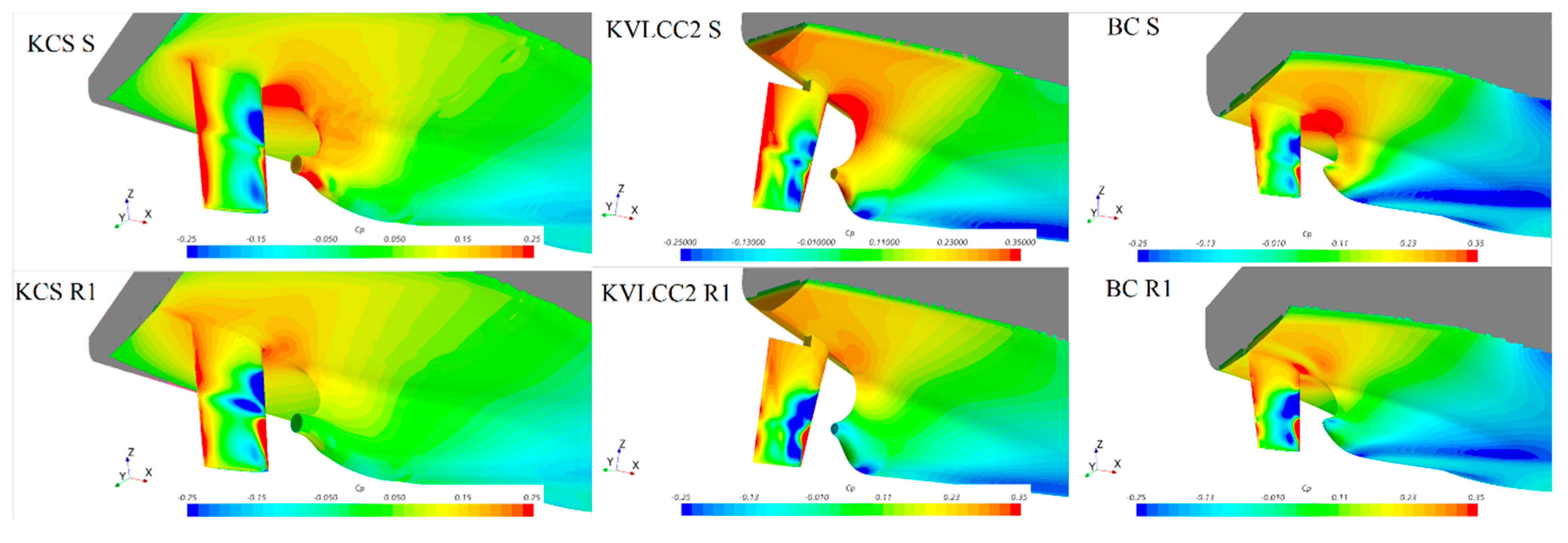
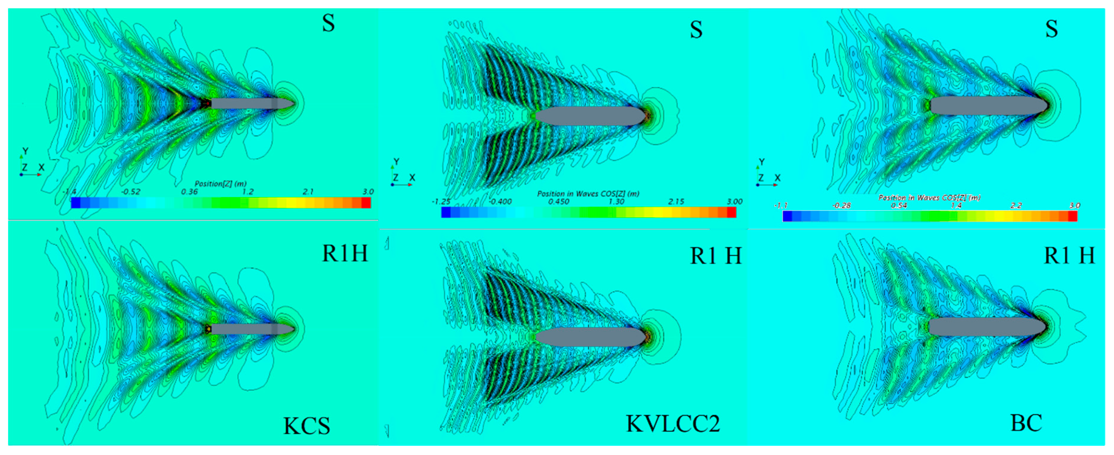
5.4. The Impact of Hard Fouling on the Flow Around Fouled Ship
6. Conclusions
Author Contributions
Funding
Conflicts of Interest
Abbreviations
| AF | antifouling |
| CFD | Computational Fluid Dynamics |
| GCI | Grid Convergence Index |
| GHG | Greenhouse Gas |
| ITTC | International Towing Tank Conference |
| MRF | Moving Reference Frame |
| PPM | Performance Prediction Method |
| OWT | Open Water Test |
| RANS | Reynolds Averaged Navier-Stokes |
| RD | Relative Deviation |
| R1-R6 | fouling conditions |
| S | Smooth surface condition |
| SPT | Self-Propulsion Test |
| VOF | Volume Of Fluid |
| HRIC | High Resolution Interface Capturing |
| FVM | Finite Volume Method |
| SST | Shear Stress Transport |
| KCS | Kriso Container Ship |
| KVLCC2 | Kriso Very Large Crude Carrier 2 |
| BC | Bulk Carrier |
| breadth (m) | |
| smooth wall log-law intercept (-) | |
| block coefficient (-) | |
| frictional resistance coefficient (-) | |
| pressure coefficient (-) | |
| total resistance coefficient (-) | |
| wave resistance coefficient (-) | |
| chord length at radius (m) | |
| propeller diameter (m) | |
| shaft diameter (m) | |
| Froude number (-) | |
| advance coefficient (-) | |
| roughness length scale (µm) | |
| form factor (-) | |
| roughness Reynolds number (-) | |
| thrust coefficient (-) | |
| torque coefficient (-) | |
| thrust coefficient in open water conditions (-) | |
| torque coefficient in open water conditions (-) | |
| length between perpendiculars (m) | |
| length of waterline (m) | |
| propeller rate of revolution (rpm) | |
| wetted surface area (m2) | |
| propeller pitch (m) | |
| mean pressure (Pa) | |
| effective power (W) | |
| delivered power at propeller (W) | |
| Reynolds number (-) | |
| propeller radius (m) | |
| frictional resistance (N) | |
| total resistance (N) | |
| height of the largest barnacle (µm) | |
| viscous resistance (N) | |
| viscous pressure resistance (N) | |
| thrust (N) | |
| time interval calculated as the ratio between ship length and speed (s) | |
| draught (m) | |
| thrust deduction fraction (-) | |
| maximum thickness at radius (mm) | |
| averaged velocity vector (m/s) | |
| non-dimensional mean velocity (-) | |
| grid uncertainty (-) | |
| numerical uncertainty in the prediction of (-) | |
| numerical uncertainty in the prediction of (-) | |
| numerical uncertainty in the prediction of (-) | |
| time step uncertainty (-) | |
| numerical uncertainty in the prediction of (-) | |
| friction velocity (m/s) | |
| speed (m/s) | |
| ship design speed (kn) | |
| non-dimensional wall distance (-) | |
| wake fraction coefficient (-) | |
| number of blades (-) | |
| percentage of the surface coverage (-) | |
| displacement (t) | |
| roughness function (-) | |
| change in certain hydrodynamic characteristic (-) | |
| displacement volume (m3) | |
| propeller efficiency behind ship (-) | |
| quasi-propulsive efficiency coefficient (-) | |
| hull efficiency (-) | |
| propeller efficiency in open water (-) | |
| relative rotative efficiency (-) | |
| von Karman constant (-) | |
| dynamic viscosity coefficient (Pas) | |
| fluid density (kg/m3) | |
| Reynolds stress tensor (N/m2) | |
| mean viscous stress tensor (N/m2) | |
| wall shear stress (N/m2) | |
| certain hydrodynamic characteristic (-) | |
| extrapolated value (-) | |
| EXP | experimental |
| EX | extrapolated |
| M | ship model |
| R | fouled surface |
| S | smooth surface |
| 1 | fine grid/time step |
| 2 | medium grid/time step |
| 3 | coarse grid/time step |
References
- Bouman, E.A.; Lindstad, E.; Rialland, A.I.; Stromman, A.H. State-of-the-art technologies, measures, and potential for reducing GHG emissions from shipping—A review. Transp. Res. D Transp. Environ. 2017, 52, 408–421. [Google Scholar] [CrossRef]
- Corbett, J.J.; Wang, H.; Winebrake, J.J. The effectiveness and costs of speed reductions on emissions from international shipping. Transp. Res. D Transp. Environ. 2009, 14, 593–598. [Google Scholar] [CrossRef]
- Poulsen, R.T.; Johnson, H. The logic of business vs. the logic of energy management practice: Understanding the choices and effects of energy consumption monitoring systems in shipping companies. J. Clean. Prod. 2016, 112, 3785–3797. [Google Scholar] [CrossRef]
- Adland, R.; Cariou, P.; Jia, H.; Wolff, F.C. The energy efficiency effects of periodic ship hull cleaning. J. Clean. Prod. 2018, 178, 1–13. [Google Scholar] [CrossRef]
- Farkas, A.; Degiuli, N.; Martić, I. Towards the prediction of the effect of biofilm on the ship resistance using CFD. Ocean Eng. 2018, 167, 169–186. [Google Scholar] [CrossRef]
- Schultz, M.P.; Bendick, J.A.; Holm, E.R.; Hertel, W.M. Economic impact of biofouling on a naval surface ship. Biofouling 2011, 27, 87–98. [Google Scholar] [CrossRef] [PubMed]
- Uzun, D.; Demirel, Y.K.; Coraddu, A.; Turan, O. Time-dependent biofouling growth model for predicting the effects of biofouling on ship resistance and powering. Ocean Eng. 2019, 191, 106432. [Google Scholar] [CrossRef]
- Farkas, A.; Song, S.; Degiuli, N.; Martić, I.; Demirel, Y.K. Impact of biofilm on the ship propulsion characteristics and the speed reduction. Ocean Eng. 2020, 199, 107033. [Google Scholar] [CrossRef]
- Yeginbayeva, I.A.; Granhag, L.; Chernoray, V. Review and historical overview of experimental facilities used in hull coating hydrodynamic tests. Proc. Inst. Mech. Eng. Part M J. Eng. Marit. Environ. 2019, 233, 1240–1259. [Google Scholar] [CrossRef]
- Uzun, D.; Ozyurt, R.; Demirel, Y.K.; Turan, O. Does the barnacle settlement pattern affect ship resistance and powering? Appl. Ocean Res. 2020, 95, 102020. [Google Scholar] [CrossRef]
- Demirel, Y.K.; Uzun, D.; Zhang, Y.; Fang, H.C.; Day, A.H.; Turan, O. Effect of barnacle fouling on ship resistance and powering. Biofouling 2017, 33, 819–834. [Google Scholar] [CrossRef] [PubMed]
- Schultz, M.P. Frictional resistance of antifouling coating systems. J. Fluids Eng. 2004, 126, 1039–1047. [Google Scholar] [CrossRef]
- Demirel, Y.K.; Song, S.; Turan, O.; Incecik, A. Practical added resistance diagrams to predict fouling impact on ship performance. Ocean Eng. 2019, 186, 106112. [Google Scholar] [CrossRef]
- Schultz, M.P. Effects of coating roughness and biofouling on ship resistance and powering. Biofouling 2007, 23, 331–341. [Google Scholar] [CrossRef]
- Demirel, Y.K.; Turan, O.; Incecik, A. Predicting the effect of biofouling on ship resistance using CFD. Appl. Ocean Res. 2017, 62, 100–118. [Google Scholar] [CrossRef]
- Farkas, A.; Degiuli, N.; Martić, I. An investigation into the effect of hard fouling on the ship resistance using CFD. Appl. Ocean Res. 2020, 100, 102205. [Google Scholar] [CrossRef]
- Song, S.; Demirel, Y.K.; Atlar, M. An investigation into the effect of biofouling on the ship hydrodynamic characteristics using CFD. Ocean Eng. 2019, 175, 122–137. [Google Scholar] [CrossRef]
- Farkas, A.; Degiuli, N.; Martić, I. Impact of biofilm on the resistance characteristics and nominal wake. Proc. Inst. Mech. Eng. Part M J. Eng. Marit. Environ. 2020, 234, 59–75. [Google Scholar] [CrossRef]
- Andersson, J.; Oliveira, D.R.; Yeginbayeva, I.; Leer-Andersen, M.; Bensow, R.E. Review and comparison of methods to model ship hull roughness. Appl. Ocean Res. 2020, 99, 102119. [Google Scholar] [CrossRef]
- Song, S.; Demirel, Y.K.; Muscat-Fenech, C.D.M.; Tezdogan, T.; Atlar, M. Fouling effect on the resistance of different ship types. Ocean Eng. 2020, 216, 107736. [Google Scholar] [CrossRef]
- Song, S.; Demirel, Y.K.; Atlar, M.; Dai, S.; Day, S.; Turan, O. Validation of the CFD approach for modelling roughness effect on ship resistance. Ocean Eng. 2020, 200, 107029. [Google Scholar] [CrossRef]
- Song, S.; Demirel, Y.K.; Atlar, M. Penalty of hull and propeller fouling on ship self-propulsion performance. Appl. Ocean Res. 2020, 94, 102006. [Google Scholar] [CrossRef]
- Leer-Andersen, M.; Larsson, L. An Experimental/Numerical Approach for Evaluating Skin Friction on Full-Scale Ships with Surface Roughness. J. Mar. Sci. Technol. 2003, 8, 26–36. [Google Scholar] [CrossRef]
- Bradshaw, P. A Note on “Critical Roughness Height” and “Transitional Roughness”. Phys. Fluids 2000, 12, 1611–1614. [Google Scholar] [CrossRef]
- Farkas, A.; Degiuli, N.; Martić, I. Assessment of hydrodynamic characteristics of a full-scale ship at different draughts. Ocean Eng. 2018, 156, 135–152. [Google Scholar] [CrossRef]
- IMO. Third IMO GHG Study 2014; International Maritime Organization (IMO): London, UK, 2014. [Google Scholar]
- Kim, W.J.; Van, S.H.; Kim, D.H. Measurement of flows around modern commercial ship models. Exp. Fluids 2001, 31, 567–578. [Google Scholar] [CrossRef]
- Hino, T.; Kenkyujo, K.G.A. Proceedings of CFD Workshop Tokyo 2005; National Maritime Research Institute: Tokyo, Japan, 2005. [Google Scholar]
- Brodarski Institute. Report 6389-M. Technical Report; Brodarski Institute: Zagreb, Croatia, 2014. [Google Scholar]
- ITTC. Recommended procedures and guidelines. In 1978 ITTC Performance Prediction Method; ITTC: Bournemouth, UK, 1999. [Google Scholar]
- Larsson, L.; Stern, F.; Visonneau, M.; Hino, T.; Hirata, N.; Kim, J. Proceedings, Tokyo 2015 Workshop on CFD in Ship Hydrodynamics; NMRI: Tokyo, Japan, 2015. [Google Scholar]
- SIMMAN. 2008. Available online: http://www.simman2008.dk/ (accessed on 1 September 2020).
- Farkas, A.; Degiuli, N.; Martić, I. Numerical investigation into the interaction of resistance components for a series 60 catamaran. Ocean Eng. 2017, 146, 151–169. [Google Scholar] [CrossRef]
- Farkas, A.; Degiuli, N.; Martić, I.; Ančić, I. Performance prediction method for fouled surfaces. Appl. Ocean Res. 2020, 99, 102151. [Google Scholar] [CrossRef]
- Tezdogan, T.; Demirel, Y.K.; Kellett, P.; Khorasanchi, M.; Incecik, A.; Turan, O. Full-scale unsteady RANS CFD simulations of ship behaviour and performance in head seas due to slow steaming. Ocean Eng. 2015, 97, 186–206. [Google Scholar] [CrossRef]
- Terziev, M.; Tezdogan, T.; Incecik, A. Application of eddy-viscosity turbulence models to problems in ship hydrodynamics. Ships Offshore Struct. 2020, 15, 511–534. [Google Scholar] [CrossRef]
- Terziev, M.; Tezdogan, T.; Oguz, E.; Gourlay, T.; Demirel, Y.K.; Incecik, A. Numerical investigation of the behaviour and performance of ships advancing through restricted shallow waters. J. Fluid Struct. 2018, 76, 185–215. [Google Scholar] [CrossRef]
- Owen, D.; Demirel, Y.K.; Oguz, E.; Tezdogan, T.; Incecik, A. Investigating the effect of biofouling on propeller characteristics using CFD. Ocean Eng. 2018, 159, 505–516. [Google Scholar] [CrossRef]
- Song, S.; Demirel, Y.K.; Atlar, M. Propeller performance penalty of biofouling: Computational fluid dynamics prediction. J. Offshore Mech. Arct. 2020, 142. [Google Scholar] [CrossRef]
- Choi, J.E.; Min, K.S.; Kim, J.H.; Lee, S.B.; Seo, H.W. Resistance and propulsion characteristics of various commercial ships based on CFD results. Ocean Eng. 2010, 37, 549–566. [Google Scholar] [CrossRef]
- Gaggero, S.; Villa, D.; Viviani, M. An extensive analysis of numerical ship self-propulsion prediction via a coupled BEM/RANS approach. Appl. Ocean Res. 2017, 66, 55–78. [Google Scholar] [CrossRef]
- Castro, A.M.; Carrica, P.M.; Stern, F. Full scale self-propulsion computations using discretized propeller for the KRISO container ship KCS. Comput. Fluids 2011, 51, 35–47. [Google Scholar] [CrossRef]
- Schultz, M.P.; Flack, K.A. The rough-wall turbulent boundary layer from the hydraulically smooth to the fully rough regime. J. Fluid Mech. 2007, 580, 381. [Google Scholar] [CrossRef]
- Flack, K.A.; Schultz, M.P.; Connelly, J.S. Examination of a critical roughness height for outer layer similarity. Phys. Fluids 2007, 19, 095104. [Google Scholar] [CrossRef]
- Farkas, A.; Degiuli, N.; Martić, I.; Dejhalla, R. Numerical and experimental assessment of nominal wake for a bulk carrier. J. Mar. Sci. Technol. 2019, 24, 1092–1104. [Google Scholar] [CrossRef]


| Fouling Condition | , μm | %SC | , μm |
|---|---|---|---|
| R1 | 7000 | 25 | 2065 |
| R2 | 5000 | 25 | 1475 |
| R3 | 7000 | 5 | 923.5 |
| R4 | 5000 | 5 | 659.64 |
| R5 | 7000 | 1 | 413 |
| R6 | 5000 | 1 | 295 |
| Parameter | KCS | KVLCC2 | BC |
|---|---|---|---|
| length between perpendiculars, | 230 m | 320 m | 175 m |
| waterline length, | 232.5 m | 325.5 m | 182.69 m |
| breadth, | 32.2 m | 58 m | 30 m |
| draft, | 10.8 m | 20.8 m | 9.9 m |
| Displacement, | 53,382.8 t | 320,750 t | 41,775 t |
| Displacement volume, | 52,030 m3 | 312,622 m3 | 40,716 m3 |
| Wetted surface, | 9645 m2 | 27,467 m2 | 7351.9 m2 |
| Block coefficient, | 0.6505 | 0.8098 | 0.7834 |
| Froude number, | 0.26 | 0.1423 | 0.2026 |
| Design speed, | 24 kn | 15.5 kn | 16.32 kn |
| Propeller center, longitudinal location from FP | 0.9825 | 0.9797 | 0.9800 |
| Propeller center, vertical location from WL | 0.62037 | 0.72115 | 0.6800 |
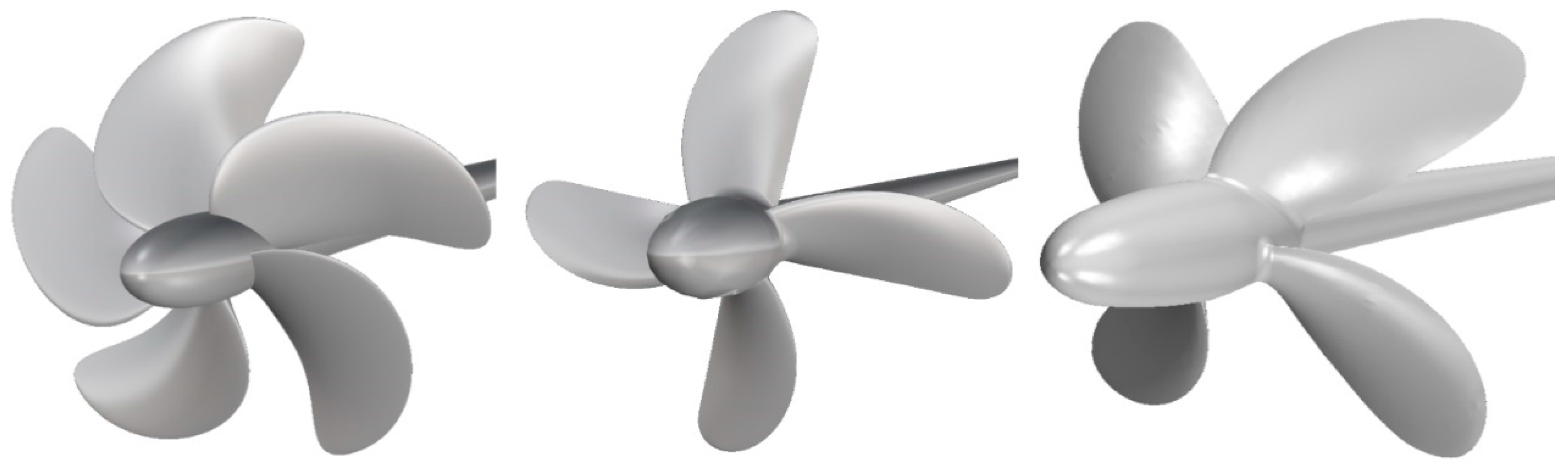
| Propeller | KP505 | KP458 | WB |
|---|---|---|---|
| propeller diameter, | 7.900 m | 9.860 m | 6.199 m |
| propeller pitch, | 7.505 m | 7.085 m | 5.294 m |
| number of blades, | 5 | 4 | 4 |
| chord length, | 2.844 m | 2.233 m | 1.633 m |
| maximum thickness of profile, | 0.132 m | 0.131 m | 0.168 m |
| Hub ratio, | 0.180 | 0.155 | 0.179 |
| Smooth Surface Condition | |||
| Simulation | KCS/KP 505 | KVLCC2/KP 458 | BC/WB |
| Coarse/Medium/Fine | Coarse/Medium/Fine | Coarse/Medium/Fine | |
| OWT | 3.50/5.10/7.10 Million | 2.40/3.30/5.30 Million | 2.20/3.50/5.00 Million |
| SPT | 2.12/4.19/8.47 Million | 1.23/2.74/5.25 Million | 0.96/2.20/5.06 Million |
| Fouling Condition R1 | |||
| Simulation | KCS/KP 505 | KVLCC2/KP 458 | BC/WB |
| Coarse/Medium/Fine | Coarse/Medium/Fine | Coarse/Medium/Fine | |
| OWT | 2.30/3.50/5.30 Million | 1.80/2.30/3.90 Million | 1.60/2.40/3.40 Million |
| SPT | 1.89/3.83/7.54 Million | 1.14/2.54/4.86 Million | 0.89/2.01/4.61 Million |
| Propeller | ||||||
|---|---|---|---|---|---|---|
| KP505 S | 0.7 | 0.18068 | 0.18047 | 0.18058 | 0.18071 | 0.092 |
| KP458 S | 0.5 | 0.18513 | 0.18576 | 0.18478 | 0.18264 | 1.443 |
| WB S | 0.56 | 0.17468 | 0.17338 | 0.17250 | 0.16758 | 3.565 |
| KP505 R1 | 0.6 | 0.20722 | 0.20665 | 0.20668 | 0.20668 | 0.001 |
| KP458 R1 | 0.4 | 0.15868 | 0.15883 | 0.15725 | 0.15698 | 0.217 |
| WB R1 | 0.4 | 0.20876 | 0.20855 | 0.20878 | 0.21098 | 1.317 |
| Propeller | ||||||
|---|---|---|---|---|---|---|
| KP505 S | 0.7 | 0.29436 | 0.29386 | 0.29387 | 0.29387 | 0.000 |
| KP458 S | 0.5 | 0.21219 | 0.21268 | 0.21169 | 0.21045 | 0.729 |
| WB S | 0.56 | 0.24312 | 0.24120 | 0.23910 | 0.23372 | 2.815 |
| KP505 R1 | 0.6 | 0.40234 | 0.40168 | 0.40249 | 0.40615 | 1.136 |
| KP458 R1 | 0.4 | 0.22703 | 0.22713 | 0.22533 | 0.22512 | 0.115 |
| WB R1 | 0.4 | 0.32578 | 0.32591 | 0.32531 | 0.32524 | 0.024 |
| Ship | Surface Condition | , MW | , MW | , MW | , MW | , % | , MW |
| KCS | S | 26.744 | 25.321 | 24.624 | 24.009 | 3.123 | 0.769 |
| R1 | 67.008 | 65.429 | 64.807 | 64.361 | 0.860 | 0.558 | |
| KVLCC2 | S | 20.172 | 17.325 | 17.850 | 18.017 | 1.174 | 0.209 |
| R1 | 58.651 | 55.524 | 55.940 | 56.036 | 0.214 | 0.120 | |
| BC | S | 7.384 | 7.267 | 6.725 | 6.573 | 2.825 | 0.190 |
| R1 | 20.778 | 21.326 | 20.301 | 19.112 | 7.318 | 1.486 | |
| Ship | Surface Condition | , rpm | , rpm | , rpm | , rpm | , % | , rpm |
| KCS | S | 100.982 | 99.686 | 99.341 | 99.225 | 0.146 | 0.145 |
| R1 | 118.374 | 117.672 | 117.376 | 117.137 | 0.255 | 0.299 | |
| KVLCC2 | S | 73.068 | 70.484 | 70.858 | 70.951 | 0.164 | 0.117 |
| R1 | 95.356 | 93.902 | 93.963 | 93.968 | 0.007 | 0.006 | |
| BC | S | 101.830 | 101.580 | 99.541 | 99.251 | 0.364 | 0.362 |
| R1 | 130.805 | 132.033 | 131.120 | 128.345 | 1.661 | 2.160 | |
| Ship | Surface Condition | , kN | , kN | , kN | , kN | , % | , kN |
| KCS | S | 1903.77 | 1877.34 | 1810.89 | 1763.46 | 3.273 | 59.281 |
| R1 | 3669.43 | 3630.48 | 3605.91 | 3557.73 | 1.670 | 60.226 | |
| KVLCC2 | S | 2276.43 | 2015.69 | 2009.71 | 2009.41 | 0.019 | 0.374 |
| R1 | 4557.62 | 4308.72 | 4390.60 | 4442.50 | 1.478 | 64.872 | |
| BC | S | 829.63 | 813.35 | 763.94 | 739.27 | 4.037 | 30.839 |
| R1 | 1616.88 | 1644.82 | 1592.13 | 1532.04 | 4.717 | 75.107 | |
| Ship | Surface Condition | , % | |||||
| KCS | S | 0.7196 | 0.7215 | 0.7293 | 0.7319 | 0.452 | 0.0033 |
| R1 | 0.5476 | 0.5442 | 0.5452 | 0.5456 | 0.094 | 0.001 | |
| KVLCC2 | S | 0.4428 | 0.4603 | 0.4573 | 0.4564 | 0.248 | 0.0011 |
| R1 | 0.3066 | 0.3128 | 0.3099 | 0.3068 | 1.257 | 0.0039 | |
| BC | S | 0.5160 | 0.5209 | 0.5328 | 0.5414 | 1.997 | 0.0106 |
| R1 | 0.3593 | 0.3580 | 0.3591 | 0.3649 | 2.041 | 0.0073 | |
| Ship | Surface Condition | , MW | , MW | , MW | , MW | , % | , MW |
| KCS | S | 25.058 | 24.918 | 24.624 | 24.355 | 1.366 | 0.336 |
| R1 | 65.020 | 65.198 | 64.807 | 64.479 | 0.633 | 0.410 | |
| KVLCC2 | S | 17.413 | 17.256 | 17.850 | 18.064 | 1.502 | 0.268 |
| R1 | 56.335 | 55.490 | 55.940 | 56.454 | 1.147 | 0.642 | |
| BC | S | 6.813 | 6.903 | 6.725 | 6.542 | 3.390 | 0.228 |
| R1 | 20.546 | 20.458 | 20.301 | 20.101 | 1.233 | 0.250 | |
| Ship | Surface Condition | , rpm | , rpm | , rpm | , rpm | , % | , rpm |
| KCS | S | 99.697 | 99.577 | 99.341 | 99.094 | 0.311 | 0.309 |
| R1 | 117.477 | 117.628 | 117.376 | 116.999 | 0.401 | 0.471 | |
| KVLCC2 | S | 70.490 | 70.249 | 70.858 | 71.255 | 0.701 | 0.496 |
| R1 | 94.492 | 93.715 | 93.963 | 94.079 | 0.154 | 0.145 | |
| BC | S | 99.638 | 100.066 | 99.541 | 97.225 | 2.909 | 2.896 |
| R1 | 130.805 | 130.529 | 130.073 | 129.374 | 0.672 | 0.874 | |
| Ship | Surface Condition | , kN | , kN | , kN | , kN | , % | , kN |
| KCS | S | 1833.25 | 1827.69 | 1810.89 | 1802.58 | 0.574 | 10.388 |
| R1 | 3611.92 | 3621.12 | 3605.91 | 3582.67 | 0.807 | 29.104 | |
| KVLCC2 | S | 2025.11 | 2018.75 | 2009.71 | 1988.26 | 1.334 | 26.816 |
| R1 | 4371.42 | 4347.51 | 4390.60 | 4444.32 | 1.529 | 67.146 | |
| BC | S | 774.04 | 784.54 | 763.94 | 742.56 | 3.499 | 26.730 |
| R1 | 1609.60 | 1597.42 | 1592.13 | 1588.07 | 0.319 | 5.077 | |
| Ship | Surface Condition | , % | |||||
| KCS | S | 0.7269 | 0.7279 | 0.7293 | 0.7319 | 0.451 | 0.0033 |
| R1 | 0.5457 | 0.5442 | 0.5452 | 0.5466 | 0.335 | 0.0018 | |
| KVLCC2 | S | 0.4596 | 0.4600 | 0.4573 | 0.4569 | 0.114 | 0.0005 |
| R1 | 0.3107 | 0.3116 | 0.3099 | 0.3082 | 0.703 | 0.0022 | |
| BC | S | 0.5312 | 0.5276 | 0.5328 | 0.5444 | 2.719 | 0.0145 |
| R1 | 0.3590 | 0.3590 | 0.3591 | 0.3591 | 0.007 | 0.0000 | |
| Ship | KCS | KVLCC2 | BC | |||
| Surface condition | , MW | , % | , MW | , % | , MW | , % |
| S | 0.839 | 3.409 | 0.340 | 1.906 | 0.297 | 4.413 |
| R1 | 0.692 | 1.068 | 0.653 | 1.167 | 1.506 | 7.421 |
| Surface condition | , rpm | , % | , rpm | , % | , rpm | , % |
| S | 0.341 | 0.343 | 0.510 | 0.720 | 2.918 | 2.932 |
| R1 | 0.558 | 0.475 | 0.145 | 0.154 | 2.331 | 1.791 |
| Surface condition | , kN | , % | , kN | , % | , kN | , % |
| S | 60.185 | 3.323 | 26.819 | 1.334 | 60.185 | 3.323 |
| R1 | 66.890 | 1.855 | 93.365 | 2.126 | 66.890 | 1.855 |
| Surface condition | , % | , % | , % | |||
| S | 0.0047 | 0.638 | 0.0012 | 0.273 | 0.0180 | 3.374 |
| R1 | 0.0019 | 0.348 | 0.0045 | 1.440 | 0.0073 | 2.041 |
| Ship | |||
|---|---|---|---|
| CFD | EX | ||
| KCS [16] | 2.081 | 2.053 | 1.376 |
| KVLCC2 [16] | 1.795 | 1.724 | 4.107 |
| BC | 2.197 | 2.296 | −4.338 |
| Ship | ||||||
|---|---|---|---|---|---|---|
| KCS | 99.341 | 100.359 | −1.014 | 24.624 | 25.511 | −3.476 |
| KVLCC2 | 70.858 | 71.417 | −0.784 | 17.850 | 18.929 | −5.701 |
| BC | 99.541 | 101.351 | −1.786 | 6.725 | 6.961 | −3.392 |
| Propulsion Characteristic | KCS | KVLCC2 | BC | |||
|---|---|---|---|---|---|---|
| EX | CFD | EX | CFD | EX | CFD | |
| 0.853 | 0.867 | 0.810 | 0.820 | 0.794 | 0.764 | |
| (1.613) | (1.199) | (−3.722) | ||||
| 0.803 | 0.773 | 0.695 | 0.668 | 0.705 | 0.653 | |
| (−3.476) | (−3.904) | (−7.418) | ||||
| 1.062 | 1.122 | 1.165 | 1.227 | 1.126 | 1.171 | |
| (5.596) | (5.310) | (3.992) | ||||
| 0.690 | 0.700 | 0.620 | 0.600 | 0.623 | 0.622 | |
| (1.485) | (−3.146) | (−0.112) | ||||
| 0.698 | 0.702 | 0.623 | 0.600 | 0.642 | 0.623 | |
| (0.565) | (−3.752) | (−2.964) | ||||
| 1.011 | 1.002 | 1.005 | 0.998 | 1.030 | 1.000 | |
| (−0.906) | (−0.626) | (−2.855) | ||||
| 0.741 | 0.787 | 0.726 | 0.736 | 0.722 | 0.729 | |
| (6.193) | (1.359) | (0.910) | ||||
| 0.750 | 0.729 | 0.472 | 0.457 | 0.565 | 0.533 | |
| (−2.786) | (−3.145) | (−5.734) | ||||
| 0.161 | 0.165 | 0.155 | 0.149 | 0.179 | 0.183 | |
| (2.954) | (−4.055) | (2.312) | ||||
| 0.275 | 0.274 | 0.187 | 0.180 | 0.251 | 0.250 | |
| (−0.477) | (−3.449) | (−0.609) | ||||
| Propeller | KP505 | KP458 | WB | ||||||
|---|---|---|---|---|---|---|---|---|---|
| Surface Condition | |||||||||
| R1 | −12.05 | 11.37 | −21.03 | −14.45 | 7.46 | −20.39 | −12.09 | 11.19 | −20.93 |
| R2 | −10.77 | 9.56 | −18.55 | −12.81 | 6.11 | −17.83 | −11.18 | 9.75 | −19.07 |
| R3 | −9.24 | 7.66 | −15.69 | −11.66 | 4.69 | −15.62 | −10.10 | 7.65 | −16.49 |
| R4 | −8.13 | 6.49 | −13.73 | −9.72 | 3.81 | −13.03 | −9.39 | 6.34 | −14.79 |
| R5 | −6.85 | 5.30 | −11.54 | −8.20 | 2.99 | −10.87 | −8.47 | 4.75 | −12.62 |
| R6 | −6.22 | 4.66 | −10.39 | −7.44 | 2.59 | −9.77 | −7.86 | 3.77 | −11.21 |
| Propulsion Characteristic | S | R1 | R2 | R3 | R4 | R5 | R6 |
|---|---|---|---|---|---|---|---|
| 0.867 | 0.852 | 0.857 | 0.858 | 0.858 | 0.856 | 0.856 | |
| −1.67% | −1.15% | −1.07% | −1.06% | −1.28% | −1.29% | ||
| 0.773 | 0.682 | 0.690 | 0.699 | 0.707 | 0.714 | 0.719 | |
| −11.7% | −10.8% | −9.56% | −8.54% | −7.64% | −6.99% | ||
| 1.122 | 1.249 | 1.243 | 1.227 | 1.214 | 1.199 | 1.191 | |
| 11.3% | 10.8% | 9.39% | 8.19% | 6.89% | 6.13% | ||
| 0.700 | 0.470 | 0.489 | 0.514 | 0.527 | 0.553 | 0.566 | |
| −32.9% | −30.2% | −26.6% | −24.8% | −21.1% | −19.2% | ||
| 1.002 | 0.998 | 1.000 | 0.999 | 1.000 | 1.001 | 1.000 | |
| −0.40% | −0.16% | −0.29% | −0.18% | −0.11% | −0.16% | ||
| 0.787 | 0.585 | 0.607 | 0.630 | 0.639 | 0.663 | 0.674 | |
| −25.6% | −22.8% | −19.9% | −18.8% | −15.7% | −14.4% | ||
| 0.729 | 0.545 | 0.560 | 0.579 | 0.592 | 0.609 | 0.620 | |
| −25.3% | −23.3% | −20.6% | −18.9% | −16.5% | −15.0% | ||
| 0.165 | 0.236 | 0.231 | 0.224 | 0.218 | 0.214 | 0.210 | |
| 42.6% | 39.6% | 35.6% | 32.0% | 29.3% | 26.8% | ||
| 0.274 | 0.436 | 0.420 | 0.402 | 0.390 | 0.374 | 0.365 | |
| 59.6% | 53.7% | 47.0% | 42.7% | 36.9% | 33.6% |
| Propulsion Characteristic | S | R1 | R2 | R3 | R4 | R5 | R6 |
|---|---|---|---|---|---|---|---|
| 0.820 | 0.812 | 0.812 | 0.813 | 0.813 | 0.814 | 0.815 | |
| −1.00% | −0.91% | −0.88% | −0.79% | −0.66% | −0.56% | ||
| 0.668 | 0.600 | 0.608 | 0.613 | 0.616 | 0.620 | 0.626 | |
| −10.1% | −9.02% | −8.19% | −7.75% | −7.17% | −6.29% | ||
| 1.227 | 1.352 | 1.337 | 1.325 | 1.320 | 1.313 | 1.302 | |
| 10.2% | 8.91% | 7.96% | 7.55% | 7.01% | 6.11% | ||
| 0.600 | 0.377 | 0.397 | 0.421 | 0.448 | 0.461 | 0.474 | |
| −37.3% | −34.0% | −29.9 | −25.4% | −23.3% | −21.1% | ||
| 0.998 | 0.997 | 1.002 | 0.998 | 0.998 | 1.003 | 1.001 | |
| −0.10% | 0.35% | −0.02% | −0.02% | 0.44% | 0.28% | ||
| 0.736 | 0.508 | 0.531 | 0.557 | 0.590 | 0.607 | 0.618 | |
| −31.0% | −27.8% | −24.4% | −19.8% | −17.6% | −16.1% | ||
| 0.457 | 0.310 | 0.322 | 0.336 | 0.348 | 0.357 | 0.367 | |
| −32.2% | −29.7% | −26.6% | −24.0% | −21.8% | −19.7% | ||
| 0.149 | 0.185 | 0.183 | 0.181 | 0.182 | 0.178 | 0.176 | |
| 24.2% | 23.4% | 21.7% | 22.4% | 20.1% | 18.2% | ||
| 0.180 | 0.242 | 0.236 | 0.230 | 0.225 | 0.220 | 0.216 | |
| 34.4% | 31.0% | 27.4% | 24.7% | 21.8% | 20.0% |
| Propulsion Characteristic | S | R1 | R2 | R3 | R4 | R5 | R6 |
|---|---|---|---|---|---|---|---|
| 0.764 | 0.787 | 0.785 | 0.782 | 0.781 | 0.779 | 0.779 | |
| 2.95% | 2.76% | 2.31% | 2.22% | 1.95% | 1.88% | ||
| 0.653 | 0.575 | 0.579 | 0.583 | 0.590 | 0.595 | 0.598 | |
| −12.0% | −11.3% | −10.7% | −9.68% | −8.89% | −8.46% | ||
| 1.171 | 1.369 | 1.356 | 1.341 | 1.325 | 1.310 | 1.303 | |
| 16.9% | 15.8% | 14.5% | 13.2% | 11.9% | 11.3% | ||
| 0.622 | 0.378 | 0.396 | 0.416 | 0.436 | 0.456 | 0.468 | |
| −39.2% | −36.4% | −33.1% | −30.0% | −26.8% | −24.9% | ||
| 1.000 | 1.000 | 0.999 | 1.001 | 0.999 | 0.999 | 1.001 | |
| −0.03% | −0.09% | 0.10% | −0.14% | −0.15% | 0.10% | ||
| 0.729 | 0.518 | 0.536 | 0.559 | 0.577 | 0.596 | 0.61 | |
| −28.9% | −26.4% | −23.4% | −20.8% | −18.2% | −16.3% | ||
| 0.533 | 0.359 | 0.371 | 0.384 | 0.397 | 0.410 | 0.418 | |
| −32.6% | −30.3% | −27.8% | −25.6% | −23.1% | −21.5% | ||
| 0.183 | 0.224 | 0.221 | 0.219 | 0.217 | 0.213 | 0.211 | |
| 22.1% | 20.8% | 19.3% | 18.4% | 16.4% | 15.1% | ||
| 0.250 | 0.338 | 0.331 | 0.321 | 0.314 | 0.306 | 0.300 | |
| 35.3% | 32.5% | 28.6% | 26.0% | 22.5% | 20.2% |
© 2020 by the authors. Licensee MDPI, Basel, Switzerland. This article is an open access article distributed under the terms and conditions of the Creative Commons Attribution (CC BY) license (http://creativecommons.org/licenses/by/4.0/).
Share and Cite
Farkas, A.; Degiuli, N.; Martić, I.; Dejhalla, R. Impact of Hard Fouling on the Ship Performance of Different Ship Forms. J. Mar. Sci. Eng. 2020, 8, 748. https://doi.org/10.3390/jmse8100748
Farkas A, Degiuli N, Martić I, Dejhalla R. Impact of Hard Fouling on the Ship Performance of Different Ship Forms. Journal of Marine Science and Engineering. 2020; 8(10):748. https://doi.org/10.3390/jmse8100748
Chicago/Turabian StyleFarkas, Andrea, Nastia Degiuli, Ivana Martić, and Roko Dejhalla. 2020. "Impact of Hard Fouling on the Ship Performance of Different Ship Forms" Journal of Marine Science and Engineering 8, no. 10: 748. https://doi.org/10.3390/jmse8100748
APA StyleFarkas, A., Degiuli, N., Martić, I., & Dejhalla, R. (2020). Impact of Hard Fouling on the Ship Performance of Different Ship Forms. Journal of Marine Science and Engineering, 8(10), 748. https://doi.org/10.3390/jmse8100748