Real-Time Prediction of Large-Scale Ship Model Vertical Acceleration Based on Recurrent Neural Network


Abstract
1. Introduction
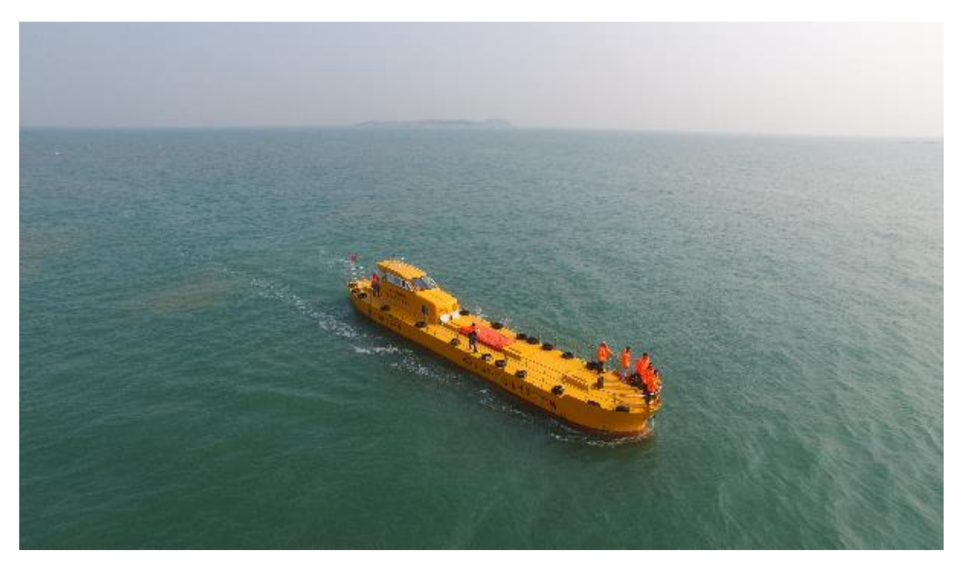
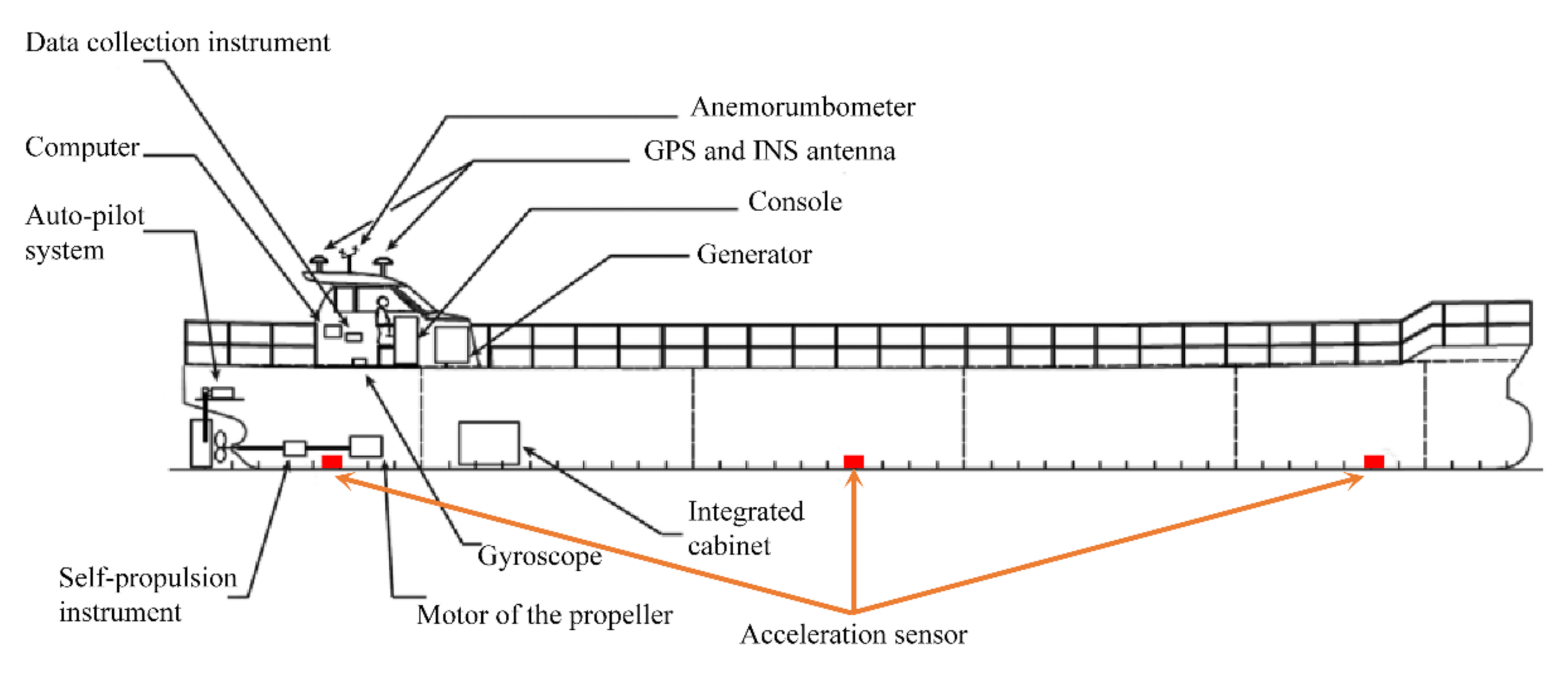
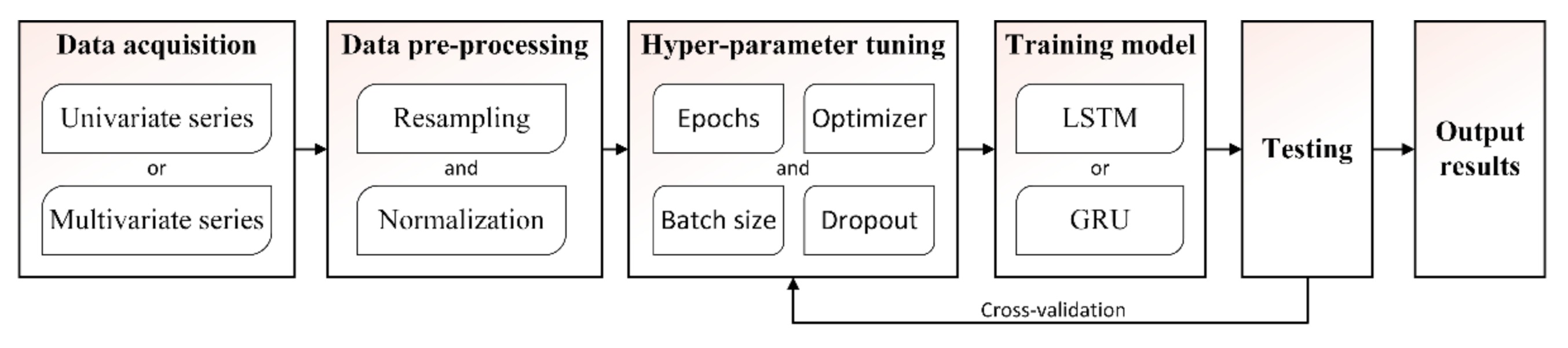
2. Data Acquisition
3. Data Pre-Processing
3.1. Resampling
3.2. Normalisation
4. Neural Network Model
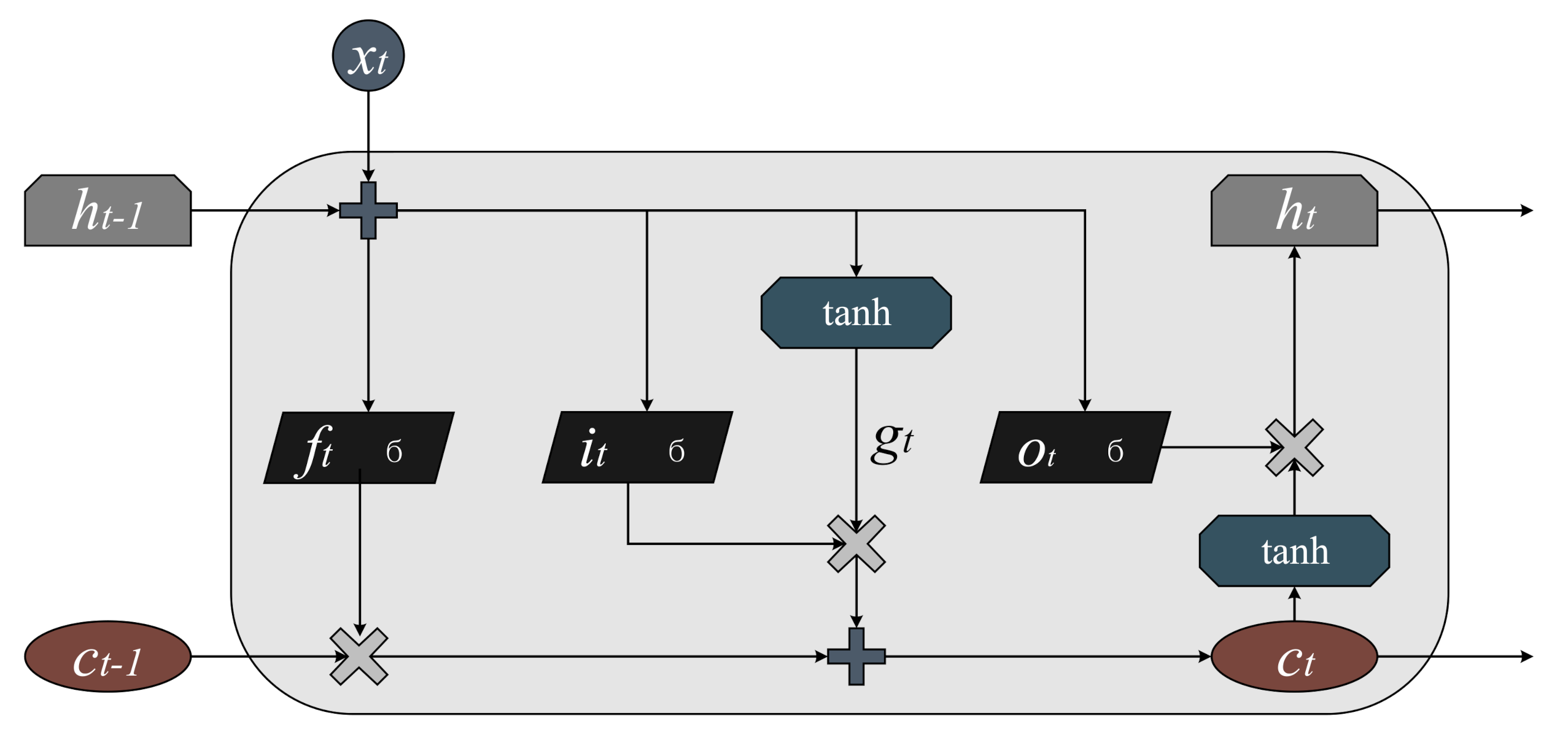
4.1. LSTM Model
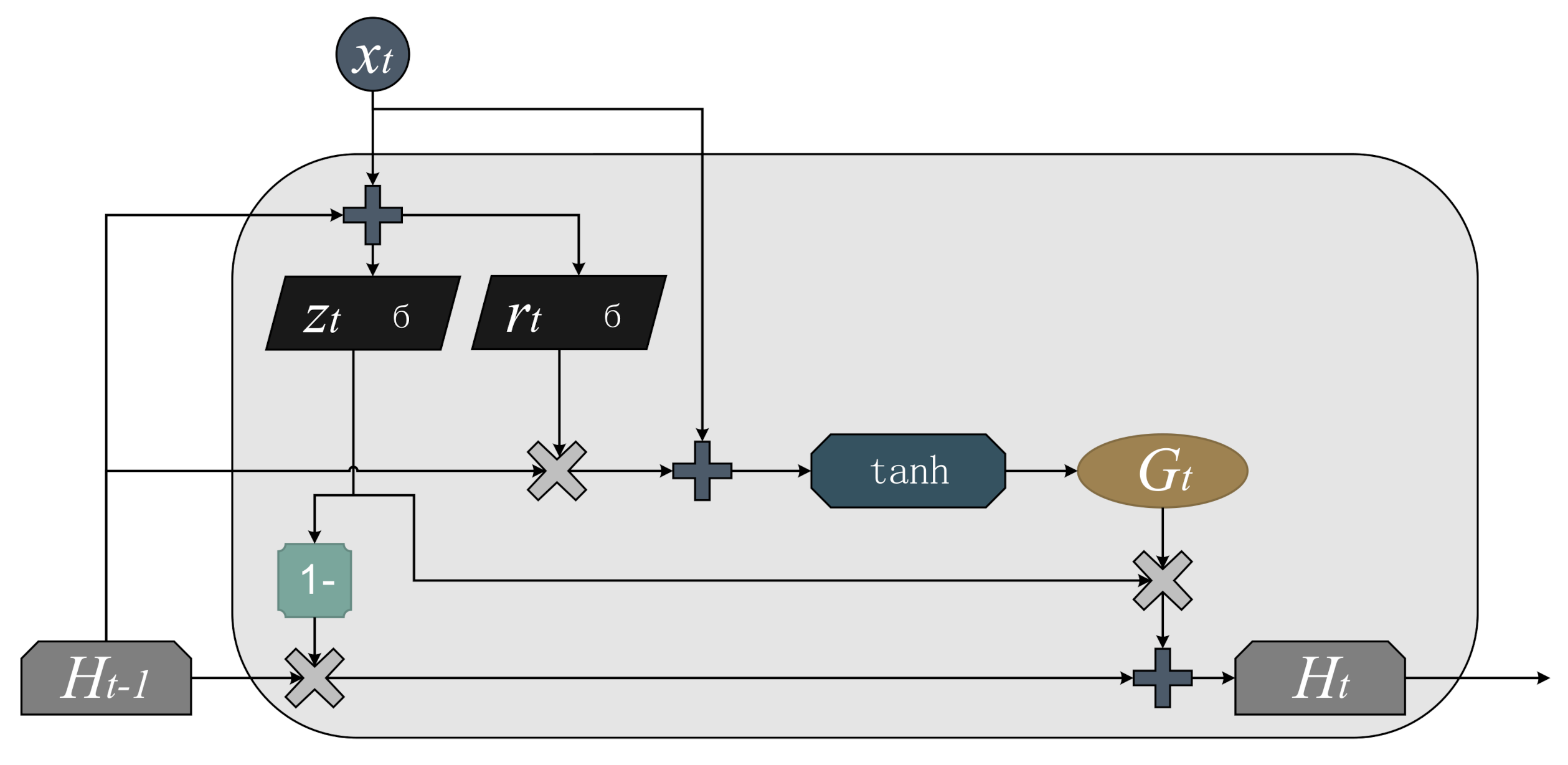
4.2. GRU Model
5. Results and Discussion
6. Conclusions
- (1)
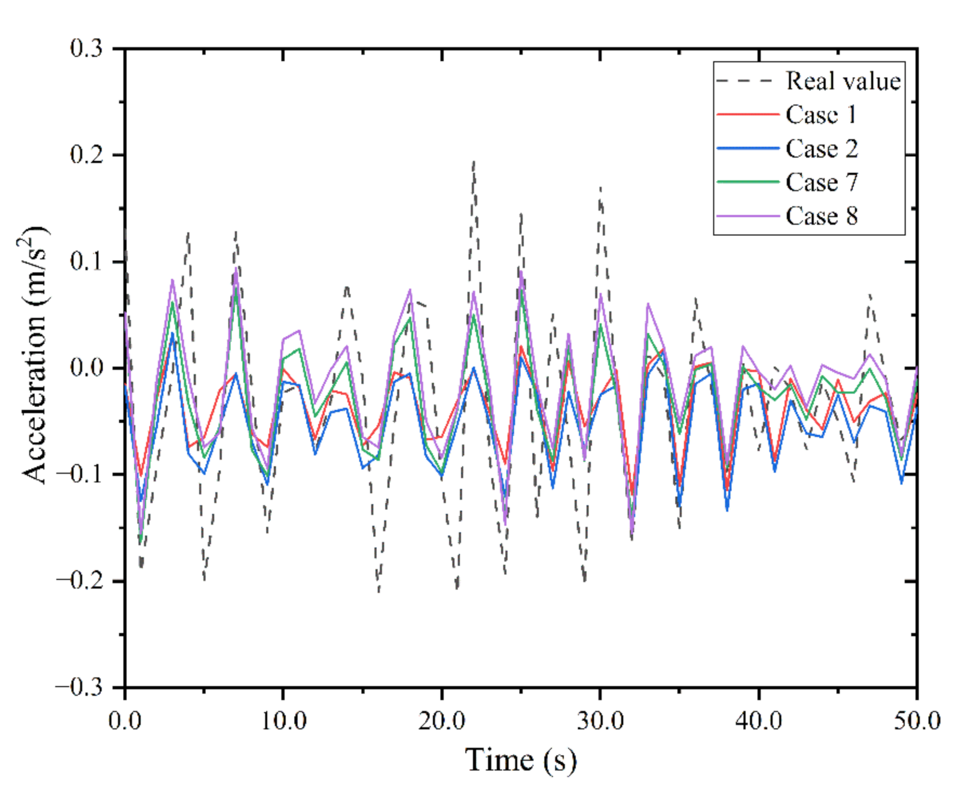
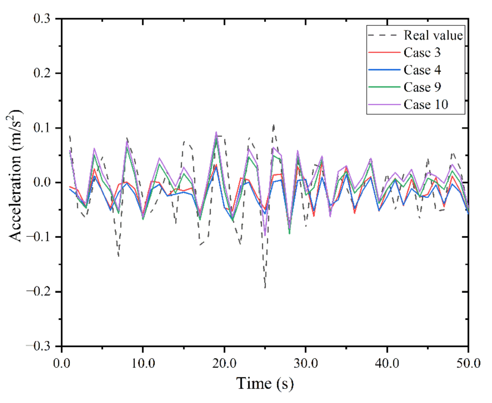
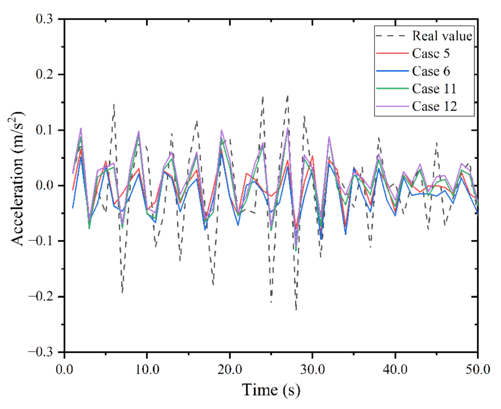
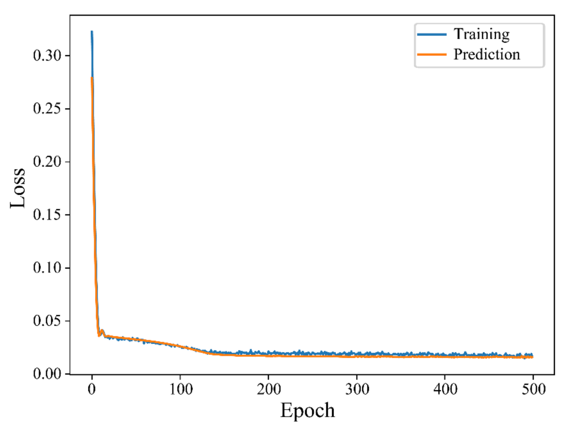
- The proposed algorithm can accurately predict the acceleration time history data of large-scale ship models at sea. In addition, the RMSE between the predicted and actual values was less than 0.1, the local prediction accuracy was affected by the high amplitude of the time history data, the final loss for neural network model training and prediction was approximately 0.02, and no over-fitting occurred.
- (2)
- The optimised multivariate time series prediction program could reduce the computing time by approximately 55% compared to that of the single-variable time series prediction program. In addition, the GRU model presented several advantages in terms of simplifying the neural network and improving the run time.
Author Contributions
Funding
Conflicts of Interest
References
- Jurdana, I.; Krylov, A.; Yamnenko, J. Use of artificial intelligence as a problem solution for maritime transport. J. Mar. Sci. Eng. 2020, 8, 201. [Google Scholar] [CrossRef]
- Li, X.; Yan, Z.; Liu, Z. Combination and application of machine learning and computational mechanics. Chin. Sci. Bull. 2019, 64, 635–648. [Google Scholar] [CrossRef]
- Marchi, E.; Vesperini, F.; Eyben, F.; Squartini, S.; Schuller, B. A novel approach for automatic acoustic novelty detection using a denoising autoencoder with bidirectional LSTM neural networks. In Proceedings of the ICASSP IEEE International Conference on Acoustics, Speech, and Signal Processing, Brisbane, QLD, Australia, 19–24 April 2015. [Google Scholar] [CrossRef]
- Shi, Z.; Xu, M.; Pan, Q.; Yan, B.; Zhang, H. LSTM-based flight trajectory prediction. In Proceedings of the IEEE 2018 International Joint Conference on Neural Networks (IJCNN), Rio de Janeiro, Brazil, 8–13 July 2018; pp. 1–8. [Google Scholar] [CrossRef]
- Karim, F.; Majumdar, S.; Darabi, H.; Harford, S. Multivariate LSTM-FCNs for time series classification. Neural Netw. 2019, 116, 237–245. [Google Scholar] [CrossRef] [PubMed]
- Srivastava, S.; Lessmann, S. A comparative study of LSTM neural networks in forecasting day-ahead global horizontal irradiance with satellite data. Sol. Energy 2018, 162, 232–247. [Google Scholar] [CrossRef]
- Wang, Z.; Yang, A.; Guo, P.; He, P. OSNR and nonlinear noise power estimation for optical fiber communication systems using LSTM based deep learning technique. Opt. Express 2018, 26, 21346–21357. [Google Scholar] [CrossRef] [PubMed]
- Gao, M.; Shi, G.; Li, S. Online prediction of ship behavior with automatic identification system sensor data using bidirectional long short-term memory recurrent neural network. Sensors 2018, 18, 4211. [Google Scholar] [CrossRef] [PubMed]
- Zhong, C.; Jiang, Z.; Chu, X.; Liu, L. Inland ship trajectory restoration by recurrent neural network. J. Navig. 2019, 72, 1359–1377. [Google Scholar] [CrossRef]
- Yang, S.; Xinya, P.; Zexuan, D.; Jiansen, Z. An approach to ship behavior prediction based on AIS and RNN optimization model. Int. J. Transp. Eng. Technol. 2020, 6, 16–21. [Google Scholar] [CrossRef]
- Hu, J.; Guo, J.; Ding, B. Automatic control of paving ship based on LSTM. In Proceedings of the 34rd Youth Academic Annual Conference of Chinese Association of Automation (YAC), Jinzhou, China, 6–8 June 2019. [Google Scholar] [CrossRef]
- Yin, J.C.; Zou, Z.J.; Feng, X. On-line prediction of ship roll motion during maneuvering using sequential learning RBF neural networks. Ocean Eng. 2013, 61, 139–147. [Google Scholar] [CrossRef]
- Besikci, E.B.; Arslan, O.; Turan, O.; Olcer, A.I. An artificial neural network based decision support system for energy efficient ship operations. Comput. Oper. Res. 2016, 66, 393–401. [Google Scholar] [CrossRef]
- Wang, C.; Zhang, X.; Cong, L.; Li, J.; Zhang, J. Research on intelligent collision avoidance decision-making of unmanned ship in unknown environments. Evol. Syst. 2018, 10, 649–658. [Google Scholar] [CrossRef]
- del Águila Ferrandis, J.; Triantafyllou, M.; Chryssostomidis, C.; Karniadakis, G. Learning functionals via LSTM neural networks for predicting vessel dynamics in extreme sea states. arXiv 2019, arXiv:1912.13382. [Google Scholar]
- Gao, D.; Jiang, Y.; Zhao, N. A novel load prediction method for hybrid electric ship based on working condition classification. Trans. Inst. Meas. Control 2020. [Google Scholar] [CrossRef]
- Nagalingam, K.K.; Savitha, R.; Mamun, A.A. An ensemble of Extreme Learning Machine for prediction of wind force and moment coefficients in marine vessels. In Proceedings of the 2016 IEEE International Joint Conference on Neural Networks (IJCNN), Vancouver, BC, Canada, 24–29 July 2016; pp. 2901–2908. [Google Scholar] [CrossRef]
- Abebe, M.; Shin, Y.; Noh, Y.; Lee, S.; Lee, I. Machine learning approaches for ship speed prediction towards energy efficient shipping. Appl. Sci. 2020, 10, 2325. [Google Scholar] [CrossRef]
- Xiros, N.I.; Kyrtatos, N.P. A neural predictor of propeller load demand for improved control of diesel ship propulsion. In Proceedings of the 2000 IEEE International Symposium on Intelligent Control. Held Jointly with the 8th IEEE Mediterranean Conference on Control and Automation (Cat. No.00CH37147), Rio Patras, Greece, 17–19 July 2000; pp. 321–326. [Google Scholar] [CrossRef]
- Kyrtatos, N.P.; Theotokatos, G.; Xiros, N.I.; Marek, K.; Duge, R. Transient Operation of Large-bore Two-stroke Marine Diesel Engine Powerplants: Measurements & Simulations. In Proceedings of the 23rd CIMAC Congress, Hamburg, Germany, 7–10 May 2001. [Google Scholar]
- Kytatos, N.P.; Theotokatos, G.; Xiros, N.I. Main Engine Control for Heavy Weather Conditions. In Proceedings of the ISME 6th International Symposium on Marine Engineering, Tokyo, Japan, 23–27 October 2000. [Google Scholar]
- Lin, J.; Zhao, D.; Guo, C.; Su, Y.; Zhong, X. Comprehensive test system for ship-model resistance and propulsion performance in actual seas. Ocean Eng. 2020, 197, 106915. [Google Scholar] [CrossRef]
- Hu, R.; Chiu, Y.-C.; Hsieh, C.-W.; Chang, T.-H.; Xue, X.; Zou, F.; Liao, L. Mass rapid transit system passenger traffic forecast using a re-sample recurrent neural network. J. Adv. Transport. 2019, 2019, 8943291. [Google Scholar] [CrossRef]
- Petneházi, G. Recurrent neural networks for time series forecasting. arXiv 2019, arXiv:1901.00069v1. [Google Scholar]
- Jozefowicz, R.; Zaremba, W.; Sutskever, I. An empirical exploration of recurrent network architectures. In Proceedings of the 32nd International Conference on Machine Learning, Lille, France, 7–9 July 2015; pp. 2342–2350. [Google Scholar]
- Qing, X.; Niu, Y. Hourly day-ahead solar irradiance prediction using weather forecasts by LSTM. Energy 2018, 148, 461–468. [Google Scholar] [CrossRef]
- Sepp, H.; Jürgen, S. Long short-term memory. Neural Comput. 1997, 9, 1735–1780. [Google Scholar] [CrossRef]
- Géron, A. Hands-on Machine Learning with Scikit-Learn and TensorFlow: Concepts, Tools, and Techniques to Build Intelligent Systems; O’Reilly: Beijing, China, 2017. [Google Scholar]
- Irie, K.; Tuske, Z.; Alkhouli, T.; Schluter, R.; Ney, H. LSTM, GRU, Highway and a Bit of Attention: An Empirical Overview for Language Modeling in Speech Recognition; Interspeech: San Francisco, CA, USA, 2016; pp. 3519–3523. [Google Scholar] [CrossRef]
- Billa, J. Dropout approaches for LSTM based speech recognition systems. In Proceedings of the 2018 IEEE International Conference on Acoustics, Speech and Signal Processing (ICASSP), Calgary, AB, Canada, 15–20 April 2018; pp. 5879–5883. [Google Scholar] [CrossRef]


| Loa, m | Lpp, m | B, m | D, m | d, m | ▽, m3 |
|---|---|---|---|---|---|
| 24.99 | 24.20 | 4.04 | 1.87 | 1.39 | 115.2 |
| Ship Speed, m/s | Wind Speed, m/s | Current Speed, m/s | Wave Period, s | Significant Wave Height, m | Sea Surface Temperature, °C |
|---|---|---|---|---|---|
| 2.0 | 0.8 | 0.3 | 4.0 | 0.1 | 21 |
| Operating System | Windows 7 64 Bits |
|---|---|
| Central processing unit (CPU) model | Intel Core i5-6500 |
| Graphics processing unit (GPU) model | NVIDIA GeForce GT 720 |
| CPU frequency, GHz | 3.2 |
| Memory size, GB | 2.0 |
| NVIDIA GPU compute capability | 3.5 |
| Cases | Neural Network Model | Input Variable | Output Variable | Total Run Time, s | RMSE | R2 |
|---|---|---|---|---|---|---|
| 1 | LSTM | a1 | a1 | 76.71 | 0.093 | 0.189 |
| 2 | GRU | a1 | a1 | 70.54 | 0.091 | 0.293 |
| 3 | LSTM | a2 | a2 | 76.67 | 0.061 | 0.116 |
| 4 | GRU | a2 | a2 | 70.62 | 0.060 | 0.154 |
| 5 | LSTM | a3 | a3 | 76.75 | 0.087 | 0.179 |
| 6 | GRU | a3 | a3 | 70.76 | 0.085 | 0.231 |
| 7 | LSTM | a1, a2, a3 | a1 | 34.01 | 0.077 | 0.510 |
| 8 | GRU | a1, a2, a3 | a1 | 32.95 | 0.079 | 0.535 |
| 9 | LSTM | a1, a2, a3 | a2 | 33.58 | 0.043 | 0.599 |
| 10 | GRU | a1, a2, a3 | a2 | 32.65 | 0.043 | 0.601 |
| 11 | LSTM | a1, a2, a3 | a3 | 33.47 | 0.069 | 0.610 |
| 12 | GRU | a1, a2, a3 | a3 | 32.92 | 0.071 | 0.617 |
© 2020 by the authors. Licensee MDPI, Basel, Switzerland. This article is an open access article distributed under the terms and conditions of the Creative Commons Attribution (CC BY) license (http://creativecommons.org/licenses/by/4.0/).
Share and Cite
Su, Y.; Lin, J.; Zhao, D.; Guo, C.; Wang, C.; Guo, H. Real-Time Prediction of Large-Scale Ship Model Vertical Acceleration Based on Recurrent Neural Network. J. Mar. Sci. Eng. 2020, 8, 777. https://doi.org/10.3390/jmse8100777
Su Y, Lin J, Zhao D, Guo C, Wang C, Guo H. Real-Time Prediction of Large-Scale Ship Model Vertical Acceleration Based on Recurrent Neural Network. Journal of Marine Science and Engineering. 2020; 8(10):777. https://doi.org/10.3390/jmse8100777
Chicago/Turabian StyleSu, Yumin, Jianfeng Lin, Dagang Zhao, Chunyu Guo, Chao Wang, and Hang Guo. 2020. "Real-Time Prediction of Large-Scale Ship Model Vertical Acceleration Based on Recurrent Neural Network" Journal of Marine Science and Engineering 8, no. 10: 777. https://doi.org/10.3390/jmse8100777
APA StyleSu, Y., Lin, J., Zhao, D., Guo, C., Wang, C., & Guo, H. (2020). Real-Time Prediction of Large-Scale Ship Model Vertical Acceleration Based on Recurrent Neural Network. Journal of Marine Science and Engineering, 8(10), 777. https://doi.org/10.3390/jmse8100777