Wireless Remote Control for Underwater Vehicles

Abstract

Nowadays, the increasing availability of commercial off-the-shelf underwater acoustic and non-acoustic (e.g., optical and electromagnetic) modems that can be employed for both short-range broadband and long-range low-rate communication, the increasing level of autonomy of underwater vehicles, and the refinement of their underwater navigation systems pave the way for several new applications, such as data muling from underwater sensor networks and the transmission of real-time video streams underwater. In addition, these new developments inspired many companies to start designing hybrid wireless-driven underwater vehicles specifically tailored for off-shore operations and that are able to behave either as remotely operated vehicles (ROVs) or as autonomous underwater vehicles (AUVs), depending on both the type of mission they are required to perform and the limitations imposed by underwater communication channels. In this paper, we evaluate the actual quality of service (QoS) achievable with an underwater wireless-piloted vehicle, addressing the realistic aspects found in the underwater domain, first reviewing the current state-of-the-art of communication technologies and then proposing the list of application streams needed for control of the underwater vehicle, grouping them in different working modes according to the level of autonomy required by the off-shore mission. The proposed system is finally evaluated by employing the DESERT Underwater simulation framework by specifically analyzing the QoS that can be provided to each application stream when using a multimodal underwater communication system specifically designed to support different traffic-based QoSs. Both the analysis and the results show that changes in the underwater environment have a strong impact on the range and on the stability of the communication link.

1. Introduction

Remotely operated vehicles (ROVs) are unmanned underwater vessels typically operated through the so-called umbilical cable, composed of an optical fiber for a broadband low-latency communication link and a power line to supply the vehicle, making it possible to manage the system in real time. However, the umbilical cable inherently limits mobility of the ROV due to cable strain and entanglement risks. Wireless ROV control would help avoid such issues by removing the need for a physical cable at the price of an increased need for ROV power autonomy and smaller data rates, a price that can be accepted only for some possible ROV applications (Figure 1).

Depending on the tasks they are designed to accomplish, ROVs can be divided into intervention-class ROVs and inspection-class ROVs [1]. The former type of vehicle, also known as work-class ROVs, is mostly used in the oil and gas industry; can weigh from 100 kg (light work-class) up to 5000 kg (heavy duty work-class); and is used for tasks such as cleaning, stabbing, and drilling as well as for carrying and operating heavy tools and sensors, such as 3D scanners for ship-hull inspection operations [2]. The latter, instead, is easier to deploy and can be used for several applications, including archaeology, coastal monitoring, search and rescue, and ship-hull and shipwreck inspection. Depending on their size, they can weigh from 3 kg (micro-ROVs) up to 120 kg (medium-size ROVs) and are typically equipped with a camera plus other optional small operational tools, such as a small manipulator or an imaging sonar. While the power consumption of intervention-class ROVs is more than 50 kW, the power required by medium-size inspection-class ROVs is less than 6 kW, and micro-ROVs require less than 1.8 kW; thus, both medium- and small-size inspection-class ROVs can be powered by lithium batteries. For some ROV applications, such as under-ice research and high-risk environment missions where the tether could be entangled, the availability of on-board batteries may be advantageous: if an emergency maneuver becomes necessary and the cable needs to be cut, this is easier thanks to its smaller size (as it does not need to carry a power supply) and the ROV can then safely resurface, behaving like an autonomous underwater vehicle (AUV). In this paper, we inspect how the use of a wireless communication system to substitute the umbilical cable would affect the quality of service (QoS) experienced by ROV pilots1 while using a medium-size battery-powered inspection-class ROV during a survey operation. In particular, we start by analyzing the required application data rates for typical services offered by inspection-class ROVs. We identify a number of operational modes which can be chosen as a function of range to support a given set of ROV services, from simple guidance and positioning up to real-time video streaming. Indeed, with the increase of the communication range, there is an exponential decrease in the achievable bit rate.

Nowadays, it is possible to establish a wireless communication link underwater through radio frequency (RF), optical, or acoustic modems [3]. These three technologies provide different performance and are used for different types of applications. Specifically, underwater RF [4,5,6] and optical communications [7,8,9] can be used for short-range broadband communication links, while acoustic signals are used for long-range low-rate communications [10,11,12]. The best communication performance is obtained when the three technologies are combined together into so-called underwater multimodal networks [3], where the best performing channels in the experienced condition are used simultaneously to achieve the desired QoS. For example, two nodes may communicate with each other via acoustics when they are more than 50 m apart and with optical modems when their distance is less than 50 m. Additionally, an RF modem can be employed to support high-rate communications when the distance between the nodes is less than 5 m and the optical channel cannot be used due to poor channel conditions (e.g., high turbidity or ambient light noise).

Also, the concept of designing a wireless hybrid ROV/AUV has already been addressed in the literature. In [13], the Woods Hole Oceanographic Institute (WHOI) presented an untethered ROV for intervention applications that make use of optical and acoustic modems to allow an ROV pilot to carry out the intended mission. In [14], we proved via simulation the possibility to exploit an underwater multimodal acoustic and optical link to pilot an inspection-class hybrid ROV/AUV, and in [15], we presented how the control range of the vehicle performing an AUV mission can be extended through a multihop acoustic network. Following the same concept, some offshore companies are currently developing commercial hybrid ROVs that can be piloted wirelessly for simple semiautonomous inspection operations [16,17]. Both our system and the WHOI untethered ROV perform best in deep water, where optical signals can reach longer distances and acoustic links are less affected by multipath [18]. On the contrary, in [19], the authors presented a wireless remote-controlled ROV for very shallow water operations: specifically, they proved through a tank test that, if the ROV is deployed in fresh water at a depth of less than 45 cm, it can be controlled through an RF wireless link in the 420–450 MHz band. In [20], the authors investigated the acoustic networking of an AUV with Autonomous Surface Vehicles (ASVs) to accomplish a common mission. After introducing the vehicle control architecture, the authors described the acoustic communication and ranging capabilities of each node and finally showed some experimental results obtained with two vehicles in the Douro river in Portugal. Recently, in [21], the authors designed an RF and acoustic wireless remote control for a BlueROV [22] vehicle. The used RF link permits a transmission rate of 1.9 kbps and a maximum range of 5 m in sea water [4]. In late 2019, the authors in [23] presented a smart buoy used as a relay for controlling and retrieving data from underwater vehicles. The buoy employs a hybrid surface RF and free-space optical link to communicate with the shore station and an underwater optical link to communicate with the underwater vehicle. The simulation model used in this paper is quite simplistic, as it does not consider solar light noise in the underwater optical link. Hydromea has recently developed an underwater drone [24] that can be piloted through a tethered system until it reaches a high-risk area, where it unplugs the cable to avoid any possibility to get entangled. From that point on, it can be controlled through a wireless optical link: indeed, both the cable connector and the drone are equipped with the LUMA optical modem [25].

This paper extends the results presented in [14,15], first by updating the review of available communication technologies, basing the remote control design and simulation results on field measurements and realistic models, and then by using realistic simulated application layers to best emulate the behavior of the vehicle and the control station.

The structure of the paper is as follows. In Section 2, we review the state-of-the-art of underwater communication technologies, paying particular attention to experimental results and selecting the most suitable underwater modems to be employed for wireless remote control. In Section 3, we analyze the data-rate requirements of an ROV control system, considering each type of traffic that needs to be transmitted. In the same section, we also define different working modes based on the level of autonomy required by the vehicle mission. Section 4 presents the simulation settings of an ROV control system designed in accordance with the observations in Section 2 and Section 3, while the whole multimodal optical and acoustic system is analyzed and evaluated in Section 5. Finally, Section 6 draws some concluding remarks.

2. Underwater Communication Technologies

Nowadays, the technologies used for underwater wireless communications are acoustics, RF, Magneto-Inductive (MI), and optical. In this section, we analyze these technologies by presenting the pro and cons of each system, some details on their expected performance, and the lessons learnt from the actual performance we experienced during sea trials.

2.1. Underwater Acoustic Communications

Developed in the late 50s of the 20th century [26], acoustic communication is certainly the most mature underwater telecommunication technology available so far. It provides long transmission ranges, up to tens of kilometers depending on the carrier frequency and the environmental conditions [10]. The modem bandwidth and its consequent communication rate depend on the carrier frequency, on the characteristics of the modem transducers, as well as on external conditions, such as noise caused by ships, wind, and marine life; the multipath; and the Doppler effect caused by the movements of the submerged nodes. For these reasons, the communication rate of an acoustic link ranges from few tens of bits per second for long-range communications up to few tens of kilobits per second for short-range links. The main disadvantage of acoustic communications are the long propagation delay caused by the low sound speed, the time variation of noise and of the channel impulse response, the presence of asymmetric acoustic links, and the poor performance in shallow water (i.e., when the water column is less than 100 m) due to signal reflections. In a mobile network deployed in shallow water, the multipath caused by signal reflections often results in link disruption, where, for instance, the communication between two nodes deployed at a depth of 1 m is established in the range of 0 up to 110 m, lost in the range of 110 up to 220 m, and established again in the range of 220 up to 290 m (Figure 2a). The link, instead, is definitely more stable in a deep-water scenario, where communication can be established up to the maximum range of the modem without link disruption (Figure 2b). Depending on the expected conditions and user needs, there is a wide set of acoustic modems in the market that can be employed in a variety of specific scenarios.

For example, to achieve a communication range of more than 4 km, a modem with a carrier frequency below 12 kHz should be used, such as Benthos ATM 960 in the low-frequency (LF) band [28], EvoLogics S2C 7/17 [29], AquaSeNT AM-D2000 [30], LinkQuest UWM3000 [31], AQUATEC AQUAmodem1000 [32], Develogic HAM.NODE [11], the Sercel MATS3G 12 kHz [33] modem, the WHOI MicroModem [12], and Kongsberg cNODE LF [34]. The transducer of most of these devices can be customized to the geometry of the channel2, and the modem bit rate can be adapted accordingly. For this reason, all LF modems can achieve a communication rate up to few kilobits per second in a vertical link in deep water, where the multipath is negligible, while in a horizontal link in very shallow water, they can reach a maximum rate of few hundreds of bits per second. Among the others, WHOI demonstrated that, in good channel conditions, it is possible to achieve a communication link of 70 to 400 km at 1 to 10 b/s in the arctic [35] by employing a carrier frequency of 900 Hz.

For communication ranges from 1 to 3 km, instead, a medium frequency (MF) modem is most suitable, as it can provide a higher bit rate. The carrier frequency of a MF modem is, depending on the manufacturer, selected between 20 and 30 kHz. All aforementioned manufacturers that produce LF devices also develop MF acoustic modems. In addition to them, other companies also supply commercial off-the-shelf products in this range, such as the Popoto Modem [36], the Applicon Seamodem [37], Sonardyne 6G [38], DSPComm Aquacomm Gen2 [39], SubNero [40], and the Blueprint Subsea [41] acoustic modem. In low-noise scenarios, a vertical communication link with an MF modem can reach a bit rate up to tens of kbps [42], depending on the modem manufacturer, while in horizontal communications in very shallow water, they can provide a communication link with a bit rate spanning from 500 bps up to few kbps.

Due to the high cost of good-quality LF and MF transducers with a wide bandwidth (the cost of the single transducer can easily exceed 2 kEUR, i.e., 2000 EURO), research and industrial prototypes of high-performance LF and MF acoustic modems are mostly developed by navy-related research institutes and companies, such as TNO [43], FOI [44], FFI [45], Wärtsilä ELAC [46], and L3HARRIS [47], that are specifically interested in very-long-range communications for surveillance applications [48]. Also, the JANUS North Atlantic Treaty Organization (NATO) standard focuses on LF and MF frequency bands [49]. In this frequency domain, some universities and civil research institutes developed some low-cost low-power products for medium- and short-range (few hundreds of meters) low-rate (few hundreds of bits per second) modems for internet of things (IoT) applications [50,51,52] by employing low-cost narrow band transducers. Some commercial low-cost MF acoustic modems (with a price of less than 2 kEUR) are also available off the shelf. For instance, the modem recently launched by DSPComm [39] has a maximum transmission rate of 100 bit/s and a nominal range of 500 m. With the same range, the Micron Data Modem developed by Tritech [53] is a low-power compact modem with a maximum data rate of 40 bps. Similar performance can be obtained with the Desert Star SAM-1 modem [54]. Finaly, DeveNET, a company that mainly produces communication and localization equipment for divers, supplies Sealink [55], an affordable and low-power acoustic modem that provides a range up to 8 km at a data rate of 80 bps.

To establish communication links of less than 500 m, a high-frequency (HF) acoustic modem with a carrier frequency of at least 40 kHz can be used. The market of HF modems is divided into two segments: low-rate acoustic modems and high-rate acoustic modems. While the former has a price below 2 kEUR and is suitable for low-rate (less than 200 bps) communication in shallow water up to a distance of 200 m [56,57,58], the latter has the same price as MF and LF acoustic modems (between 8 and 10 kEUR, depending on depth rate requirements) and can be used for sending a still-frame slide-show-like video feedback from an underwater vehicle [43,59,60,61,62] to a control station, as they can perform transmissions with a bit rate of more than 30 kbps [29]. In this paper, we focus on this last type of modem in order to achieve the best performance possible despite the higher price. Indeed, they can easily achieve a bit rate of more than 30 kbps in vertical links, and in horizontal communications in very shallow water, they can still provide a rate of at least 2 kbps.

Although several high-rate acoustic modems are available in the literature, only a few of them are commercial off-the-shelf products. The maximum rate of a LinkQuest [31] modem is 35.7 kbit/s (with a directional beam pattern), while EvoLogics S2CM HS [29] is the off-the-shelf modem that provides the highest bit rate (62.5 kbit/s up to 300 m in good channel conditions, although its actual maximum throughput would typically be about 30 kbit/s). This last modem has been used in [61] to perform in-tank low-quality video streaming, where the transmission bit rate selected by the modem during its initial handshake phase [63] was 31.25 kbps and the actual throughput obtained 20 kbps. In good channel conditions, this performance can also be obtained with other EvoLogics models, such as S2C 48/78 and S2C 42/65. While the former is optimized for horizontal communications, the latter is suitable for vertical links. S2C HS, instead, has an omnidirectional transmitter and, therefore, is more suitable for being installed in an AUV or in an ROV. Modems that can provide a higher bit rate are either university noncommercial systems [59,62,64,65] or company prototypes waiting for a bigger market demand before becoming available off the shelf [66]. The Marecomms Roboust Acoustic Modem (ROAM), recently developed in partnership with Geospectrum, achieves a throughput of 26.7 kbps at a distance of 600 m while operating in the HF band in shallow water. A test has been performed in the presence of Doppler as the nodes were floating randomly with a speed between 0.5 and 1 knot [67]. With the new version of the modem, the manufacturer expects to achieve 50 kb/s within a range of 1 km. This modem is expected to become available on the market by late 2020 to early 2021. The ROAM modem can also operate in the MF band, providing a bit rate of 13 kbps.

The most representative underwater acoustic modems with omnidirectional beam patterns that can also be employed for communications in shallow-water scenarios are summarized in

Table 1. Performance figures of some acoustic modems with omnidirectional beam patterns.

	Manufacturer and Model	Max Range	Bit Rate
LF	Sercel MATS3G 12 kHz [33]	15 km	{20, 200} bps secure data with coding, {0.8, 7.4} kbps high rate with no coding
	EvoLogics S2C R 7/17 [29]	7 km	{1, 7} kbps raw bit rate with no coding, {0.6, 4} kbps net data rate with coding
	WHOI MicroModem [12]	[6, 11] km	{0.2, 5.4} kbps in vertical links [68]
	LinkQuest UWM10000 [31]	7 km	5 kbps raw bit rate, 2 kbps payload data rate
	Kongsberg cNODE LF [34]	few kms	up to 4.5 kbps
	Benthos ATM 960 LF [28]	6	{0.08, 2.4} kbps
	AQUATEC AQUAmodem1000 [69]	10 km	{0.1, 2} kbps
	AquaSeNT AM-D2000 [30]	5 km	{0.375, 1.5} kbps
	DiveNET: Sealink R [55]	2.5 km	{0.56, 1.2} kbps in shallow water
	Develogics HAM.NODE [11]	30 km	145 bps
	DiveNET: Sealink {C,S} [55]	8 km	80 bps in shallow water
MF	Sercel MATS3G 34 kKHz [33]	5 km	{20, 300} bps secure data with coding, {1, 24.6} kbps high rate with no coding
	LinkQuest UWM2000 series [31]	1 km	17.8 kbps raw bit rate, {0.3:6} kbps payload data rate
	Subnero WNC [40]	[3, 5] km	15 kbps
	EvoLogics S2C R 18/34 [29]	3.5 km	{1, 13.9} kbps raw bit rate with no coding, {0.6, 9} kbps net data rate with coding
	Popoto Modem [36]	[1, 8] km	{0.08, 10} kbps
	AquaSeNT AM-OFDM-13A [30]	5 km	{1.5, 9} kbps
	Sonardyne 6G [38]	1.5 km	{0.2, 9} kbps
	Kongsberg cNODE MF [34]	1 km	up to 4.5 kb/s
	Benthos ATM 960 MF, band C [28]	1.5 km	{0.08, 2.4} kbps, 15 kbps possible in very quiet deep ocean environments
	Applicon Seamodem [37]	100 s of m	{0.75,2} kbps
	DSPComm Aquacomm Gen2 [39]	8 km	{0.1, 1} kbps
	Blueprint Subsea X150 USBL Beacon[41]	1 km	100 s bps
	DiveNET: Sealink M [55]	1 km	80 bps
HF	Rutgers MIMO modem [62]	10 s of m	{100, 250} kbps
	Northeastern SEANet prototype [65]	10 s of m	{41, 250} kbps
	BaltRobotics Prototype [66]	[100, 200] m	{1, 115} kbps
	MIT Prototype [59]	200 m	100 kbps
	FAU Hermes modem prototype [64]	150 m	87.7 kbps
	EvoLogics S2C M HS [29]	300 m	{2, 62.5 kbps raw bit rate with no coding, {1.2, 35} kbps net data rate with coding
	Marecomms ROAM Prototype [67]	0.6 km 1 km expected	26.7 kbps actual throughput in shallow water 50 kbps expected in the new version
	AHOI modem [56]	200 m	200 bps
	Waterlinked M64 [57]	200 m	64 bps

.

2.2. Optical Communications

Although acoustic modems are the typical solution for underwater communications, their bandwidth is very limited. The need for high-speed communications in an underwater environment has pushed the realization of optical devices that can transmit data within short distances at a bit rate on the order of one or more Mbps (up to few Gbps at very short ranges, depending on the model and the water conditions). Indeed, unlike acoustic communications, optical communications are more suitable for ranges up to 100 m, especially in deep dark waters, and are not affected by multipath, shipping, and wind noise, as their performance mainly depends on water turbidity and sunlight noise [70]. In fact, high turbidity scatters and attenuates the optical field, whereas ambient light may become a significant source of noise, making transmissions close to the sea surface more difficult. The turbidity coefficient, called the attenuation coefficient, is composed of the sum of scattering and absorption coefficients. The former depends on the quantity of particles, such as plankton, dissolved in the water. The plankton exists due to the chlorophyll effect, that happens only where solar light reaches the medium, i.e., in shallow water, up to a depth of 100 m. The latter, instead, is an inherent optical property of the medium. Blue and green lights, which have wavelengths of 470 and 530 nm, respectively, are the most widely used for underwater optical communication [71], as these wavelengths are the least attenuated in deep and shallow water, respectively. Intuitively, in order to understand which of the two wavelengths is less attenuated in a certain scenario, we just need to observe the color of the water in the presence of white light (e.g., sunlight). If the color of the water is blue, the best wavelength to use is around 470 nm (that is the typical case of a deep water deployment); otherwise, if the water color is green, wavelengths around 530 nm should be employed (that is the typical case of deployment close to the surface).

Similar to acoustic modems, optical transceivers are also designed to perform best in some scenarios; therefore, the best optical modem that outperforms all others in all possible conditions does not exist. Specifically, we can divide the optical modems into models composed of a light emitting diode (LED)-based transmitter designed for hemispherical communications [8,25,72,73] and models composed of a high-directional laser-based transmitter [74,75,76,77,78,79]. Although the latter achieves a throughput from 10 to 100 times higher than the former, we focus on LED-based modems, as laser-based transmitters require perfect alignment between the transmitter and receiver, a condition that a mobile vehicle can fulfill only during a docking operation or if the modems are equipped with beam-steering capabilities, such as the SA Photonics Neptune modem [80]. The latter, however, is not an off-the-shelf product, i.e., it is custom built to order, with a significantly higher price compared to other commercial products.

We can also divide the optical modems into models tailored for dark water medium range (MR) communications (up to 100 m) [7,25] and devices designed for short-range (SR) communications in high ambient light environments [9]. In the MR class, we can find Sonardyne BlueComm 200 [7], equipped with a very sensitive receiver based on a photomultiplier. This modem achieves a hemispherical transmission rate of 10 Mbps up to a distance of 100 m, but only in deep, dark waters. The same modem would perform poorly in the presence of light noise due to saturation of the receiver: for this reason, Sonardyne designed an ultraviolet version of this modem, able to achieve a maximum range of 75 m even in the presence of some ambient light. Still, from our experience, both models are unable to establish a communication link when deployed a few centimeters above the sea surface during daytime. Similar issues have been experienced with Hydromea Luma 500ER [25], able to cover, in good conditions, more than 50 m with a bit rate of 500 kbps (beam pattern 120${}^{\circ }$); the Ifremer optical modem [73], that can communicate at a similar range with a bit rate of 3 Mbps; and the early-stage version of the ENEA proof of concept (PoC) prototype [81]. Also, the AquaOptical modem developed by MIT [72] can perform MR communications in low solar noise conditions by reaching a maximum range of 50 m with a rate of 4 Mbps. The beam patterns of both the Ifremer and MIT modems are 100${}^{\circ }$, while the ENEA optical modem is omnidirectional. Customized LED-based MR optical modems are developed by Penguin ASI [82,83]; the maximum performance of their system is in the order of 100 s of Mbps at hundreds of meters but comes at the price of very bulky and expensive modems that are only suitable for extremely specialized applications, such as deployment in heavy-size working-class ROVs or similar vehicles.

Models designed for SR communications, instead, typically overcome the ambient light noise issue by employing a noise-compensating mechanism to avoid receiver saturation, at the price of lower bit rate and range. This mechanism typically consists of measuring the average noise at the receiver and of injecting a signal with equal intensity but opposite sign at the receiver unit. BlueComm 100 [7], for instance, can be used in all water conditions, including shallow water in daytime to transmit at a rate of 5 Mbps in SR at a maximum distance of 15 m. Its beam pattern is 120${}^{\circ }$. Similarly, the Sant’Anna OptoCOMM modem [8] can establish a 10-meter communication link at a speed of 10 Mbps, when both the receiver and transmitter are deployed just half a meter below the sea surface. They use optical lenses to reduce the beam aperture angle to 20${}^{\circ }$ and to reduce the receiver field of view to 70${}^{\circ }$ to limit sunlight noise. Also, ENEA developed a solar light noise-cancellation mechanism for their new version of the optical modem: preliminary results declared by ENEA proved that their new prototype can now communicate in high ambient light conditions, at the price of a reduced bit rate. Another commercial off-the-shelf optical modem for SR is the AQUAmodem Op1 [9], which achieves 80 kbps at 1 m, with a beam pattern of 34${}^{\circ }$. The company declares that the modem is affected by direct sunlight noise but is generally robust to low sources of ambient light noise, as it can be used in the presence of ROV lights without compromising the communication link. The same happens for the CoSa optical modem [5], able to reach 2 Mbps at up to 20 m, with a transmitting beam aperture angle of 45${}^{\circ }$ and a receiver field of view of 90${}^{\circ }$. Another low-cost modem that is quite robust to sunlight noise is the optical modem developed by IST [84] that can reach 200 kbps at a maximum distance of up to 10 m and, different from the other modems presented so far, uses green instead of blue LEDs, as it is specifically tailored for shallow-water operations. This modem uses optical lenses to reduce the beam aperture angle to 12${}^{\circ }$ and an optical filter to reduce sunlight noise.

The most representative underwater optical modems are summarized in

Table 2. List of performance figures for representative optical modems.

	Manufacturer and Model	Max Range	Bit Rate
Laser	FUDAN modem [76]	34.5 m	2.70 Gbps
	Oceanit ultra [78]	100 m	1 Gbps
	USTC modem [77]	100 m	500 Mbps
	Sonardyne BlueComm 5000 [75]	7 m	500 Mbps
	SA Photonics Neptune [80]	200 m	200 Mbps customized, with beam steering capabilities
	MC100  [74]	10 m	95 Mbps
	JAMSTEC modem [79]	50 m	20 Mbps
LED SR	Sant’Anna OptoCOMM [8]	10 m	10 Mbps
	Sonardyne BlueComm 100 [7]	15 m	5 Mbps
	CoSa optical [5]	20 m	2 Mbps
	ENEA PoC [81]	1 m	2 Mbps
	IST Medusa Optical Modem [84]	10 m	{20, 200} kbps
	Aquatec AQUAmodem Op1 [9]	1 m	80 kbps
LED MR	Penguin Automated Systems [82]	[10, 300] m	{1.5, 100} Mbps custom
	Sonardyne BlueComm 200 [7]	120 m	10 Mbps
	Sonardyne BlueComm 200 UV [7]	75 m	10 Mbps
	MIT AquaOptical modem [72]	50 m	4 Mbps
	Ifremer optical modem [73]	60 m	3 Mbps
	Hydromea Luma 500ER [25]	50 m	500 kbps

.

2.3. Radio Frequency and Magneto-Inductive Communications

Also, electromagnetic radio frequency and magneto-inductive communications can be used underwater. Compared with acoustic and optical waves, RF waves can perform a relatively smooth transition through the air–water interface [85]. This benefit can be used to achieve cross-boundary communication: for instance, the authors in [19] used this concept to pilot an ROV deployed up to 45 cm below the water surface. Another advantage is that RF and MI are almost unaffected by water turbulence, turbidity, misalignment between transmitters and receivers, multipath, and acoustic and solar noise, that are the main causes of poor performance for either optical or acoustic modems when used in practical scenarios. For these reasons, when in range, RF and MI can provide a much more stable link than optical and acoustic communications, with less disruptions; thus, in our opinion, they should be preferred to the other media whenever the bit rate and the range required by the application can be supported. However, their communication range is usually limited to no more than a few meters. Inductive modems [86,87,88], for instance, are often deployed in mooring systems [89,90], as they enable communication over jacketed mooring lines and can be used to retrieve data from instruments such as Conductivity, Temperature, and Pressure sondes (CTDs) and Acoustic Doppler Current Profilers (ADCPs) by substituting physical connectors and the need for dedicated cables for communication. These modems generate a low-frequency signal that travels in the mooring line and can only substitute mechanical connectors for low-rate communications (up to 5 kbps). Also RF modems [5,91] can be used to replace the mechanical connector of cables in very short ranges, but they provide broadband communications (up to 100 s of Mbps) and thus can support high-rate-demanding applications, such as real-time control and high-quality video streaming. For example, Hydromea uses an RF connector in the umbilical cable of the EXRAY ROV [24], where the vehicle’s tether can be disconnected to perform an autonomous mission before being reconnected again. Also, in this case, the communication range is in the order of few centimeters. WiSub supplies the Maelstrom connector [92], able to support both power and data transfer via RF. Communication based on a microwave link has a rate of 100 Mbps up to a distance of 5 cm between the connectors. Similar devices are sold also by Blue Logic [93]. Broadband RF modems can also be employed in docking stations to quickly download data from an AUV [94]. For instance, the WFS Seatooth S500 [91] RF modem provides a bit rate up to 100 Mbps up to a range of 10 cm, and the Lubeck University of Applied Science developed the CoSa underwater WiFi [5], with a rate of 10–50 Mbps up to 10 cm.

These examples prove how RF communications can achieve high transmission bit rates underwater, although their communication range is very limited. Indeed, RF communications suffer from RF interference and are prone to very strong attenuation in salty waters, where the conductivity of the medium is larger than in fresh waters. A range up to a few meters (SR) can be reached with RF modems, at the price of a lower bit rate. For example, INESC Tec developed a dipole antenna prototype [6] to support 1 Mbps communication at 1 m, and the Lubeck University of Applied Sciences developed a dipole [5] antenna to communicate with a rate of 0.2 to 1 Mbps and a range of 1-8 m, depending on water conditions (i.e., 1 meter in salty water and 8 m in fresh water).

Although in air MI communication is outperformed by RF modems, as the latter can achieve a higher bit rate and a longer range, underwater MI modems are almost unaffected by the change of medium while the electrical field is strongly attenuated. Indeed, MI modems are proven to reach a bit rate of a few kbps at tens of meters, both in air and underwater [95]. Dalhousie University developed an MI prototype that achieves 8 kbps at 10 m [96], to perform low-rate low-latency communications. With MI modems, longer distances can be achieved at the price of a lower bit rate. For instance, the authors in [95] established a directional link with a maximum range of 41 m and an omnidirectional link with a range of 26 m. Both links provide data rates of 512 bps. With their new modem design recently presented in [97], they were able to achieve 1 kbps at a 40-m distance with an omnidirectional beam pattern. Nearly 20 years ago, the authors in [98], instead, demonstrated a 153-bps communication link at a distance of 250 m and a 40-bps communication link at a distance of 400 m.

Very-low (VLF) and extremely-low radio frequency (ELF) signals have been extensively used during the cold war to communicate from inland control stations to submarines [99]. The drawbacks of these systems are the low rate and the need for a very large and high-power-consuming inland antennas. Indeed, VLF can provide a 300 bps one-way communication link from shore to the submarine up to a distance of 20 m below the sea surface and requires a broadcast inland antenna with a size between 300 m and 2 km [99]. For example, the Sweden Grimeton Radio Station [100] uses a set of antennas that are 1.9 km long, each with an RF power peak of 200 kW.

ELF can also be used to communicate from land to submarines (one way): they reach up to 1 bps [101] at a range of several hundreds of meters below the sea surface but require a grounded wire inland antenna (ground dipole) with a size of several tens of kilometers and a transmission power in the order of millions of watts. Due to the high cost of deployment, US, Russia, India, and China are the only nations known to have constructed ELF communication facilities. For instance, the US ELF system employed a ground dipole antenna 52 km long [102] while the Russian system used an antenna 60 km long [103]. This system has been typically used to signal one-way coded messages to the submarine’s commander to resurface to receive more information via other means.

Both VLF and ELF technologies are not applicable to ROVs and AUVs but only to submarines due to their very large size and demanding power consumption.

The most representative underwater MI and RF communication systems are summarized in

Table 3. List of performance figures for representative radio frequency (RF)/magneto-inductive (MI) underwater modems.

	Manufacturer and Model	Max Range	Bit Rate
(E)VLF-RF	VLF (3–30) kHz [99,100]	20 m below the sea surface, inland antenna size = 2 km	300 bps one way, from land to underwater
	ELF (3–300) Hz [102,103]	hundreds of meters below the sea surface, inland ground dipole size = [52, 60] km	1 bps one way, from land to underwater
MI	Dalhousie Univ. Prototype [96]	10 m	8 kbps
	inductive modems for mooring lines [86,87,88]	up to few kilometers from tx using the mooring line, few cm from the mooring line	{1, 2} kbps
	MST Prototype [97]	40 m	1 kbps
	CSS/MISL Prototype [98]	[250, 400] m	{153, 40} bps
RF	WiSub Maelstrom [92]	5 cm	100 Mbps
	CoSa WiFi [5]	10 cm	{10, 50} Mbps
	WFS Seatooth S500 [91]	10 cm	10 Mbps
	INESC TEC Dipole [6]	1 m	1 Mbps
	CoSa EF Dipole [5]	[1, 8] m	{0.2, 1} Mbps
	WFS Seatooth Mark IV SR [4]	[5, 7] m	2.4 kbps
	WFS Seatooth Mark IV MR [4]	[30, 45] m	100 bps

.

2.4. Modem Selection and Considerations

According to the technology comparison presented in this section and summarized in Figure 3, we can conclude that optical technologies are the preferred choice up to a distance of about few tens of meters (100 m in very good conditions) whereas acoustics would be the preferred choice from that point onward. We also note that RF and MI modems are consistently outperformed by optical or acoustic modems, although they have the advantage that their communication is not prone to environmental characteristics (unlike acoustic and optical).

The optical modem considered in this paper is BlueComm 200, that has a hemispherical beam pattern and is able to transmit at a speed of 10 Mbps at a range up to 100 m in good channel conditions, such as those considered in this paper. For different scenarios, when choosing which modem to use, it should be considered that the BlueComm 200 modem is strongly affected by noise due to sunlight and external lights, and for this reason, Sonardyne supplies it together with an ROV lighting system that does not affect the modem performance. Indeed, BlueComm 200 can be used only in deep-water scenarios or during night operations in shallow water. If the ROV needs to be operated in shallow water during daytime, a different model tailored for shorter ranges in these conditions should be selected, like BlueComm 100, that achieves a maximum range of 15 m and a maximum rate of 5 Mbps even in the presence of sunlight, or BlueComm 200 UV, that still suffers from direct sunlight but is robust against ROV lighting systems.

One of the most important things to take into account when selecting multiple acoustic modems to be used in the same network is to avoid interference between the different devices. For instance, if both LF and MF acoustic modems need to be used in the same system, the maximum working frequency of the LF modem must be smaller than the minimum working frequency of the MF modem to avoid bandwidth overlap. Moreover, some guard between the bandwidths of the modems should be provided, as the drop of the transducer sensitivity outside the modem bandwidth is usually not vertical: for example, EvoLogics S2C 7/17 should not be used along with EvoLogics S2C 18/34 because the bandwidths of the two modems are spaced apart only by 1 kHz. In this work, we cannot analyze the characteristics of all transducers of each modem (as most companies do not provide this information); thus, we assume that two modems can be used together if their bandwidths are spaced apart by at least 5 kHz.

When designing deployment with an underwater vehicle, also the interference between modems and the acoustic localization systems, such as ultra-short baseline (USBL) and long baseline (LBL) acoustic positioning systems [104], used to track the vehicle position along the whole mission must be avoided. A USBL is composed of two components: a transceiver, usually deployed from a control station with a well-known position, such as a ship, and a transponder, installed on the underwater vehicle that needs to be tracked. The former is equipped with an array of at least four hydrophones, used to determine the target position from the range and bearing obtained from the acoustic signal received by the latter. Specifically, the transceiver sends an acoustic pulse (interrogation) to the transponder that responds with another acoustic pulse (reply) immediately, so the transceiver can triangulate the position of the transponder by means of its hydrophone array. In case of bandwidth overlap, the acoustic pulses sent by the USBL may interfere with the acoustic communications: to overcome this issue, some companies [41,105] provide the possibility to perform low-rate communication (up to few hundreds of bits per second) with their USBL systems. Some modem manufactures, instead, provide a version of their modem that incorporates a USBL [28,29,31,34,38,47,55], where the transponder is just a normal unit of the modem programmed to answer the USBL request and the transceiver is a modified version of the modem that includes the hydrophone array into the modem transducer.

An LBL system, instead, uses a network of sea-floor-mounted baseline transponders as the reference point for navigation. The exact coordinates of the baseline transponders are known, and they are used for determining target positions. Baseline transponders reply to acoustic interrogation signals from target-mounted transponders with their own acoustic pulses, allowing a target to calculate its own position by measuring the distance between itself and each transponder of the baseline array. Although the deployment of an LBL, that typically requires at least four baseline transponders plus the target transponder, is more expensive than the deployment of a USBL, it provides a higher positioning precision and is often used in oil and gas fields. In addition, the LBL transponder can either be specifically manufactured for positioning [105] or can be a regular acoustic modem with positioning capabilities [12,28,29,31,34,38,40,55,56,57].

The modems equipped with USBL or LBL functionalities are able to switch between positioning and data modes or provide an automatic protocol that performs tracking of the vehicle along with the communication, at the price of a throughput reduction between 10% and 20%. In our design, the longest range acoustic modem should also provide either LBL or USBL capabilities.

One of the main disadvantages of LF acoustic modems when used in ROV and AUV operations is the fact that they are strongly affected by noise caused by the propellers of ships and vessels [106]. From our tests, we indeed discovered that, in a network deployed 40 m from a cargo ship docked in a port, a long-range EvoLogics S2C 7/17 modem reaches only the same transmission range as an EvoLogics S2C HS (i.e., 200 m) because the noise level of the former is very close to the saturation level of its transducer while the latter is almost unaffected due to its high-frequency bands. Indeed, HF acoustic signals mainly suffer from the noise caused by wind-driven waves and not by shipping noise [10]. Another reason why MF and HF modems are used more often in small AUVs and ROVs than LF modems is because the integration of LF modems in small vehicles can be complex or even impossible due to the large size of their transducer, that has a diameter of at least 12 cm and a total weight that can easily exceed 5 kg. MF and HF modems, instead, usually have a total weight of less than 2.5 kg and a transducer diameter of less than 6 cm.

The acoustic modems selected for the wireless remote control designed in this paper are the Subnero WNC and the EvoLogics S2C HS, both equipped with an omnidirectional transducer, the former operating in the MF bandwidth with LBL capabilities and the latter operating in the HF bandwidth.

3. Requirements and Definition of Working Modes for ROV Control

In this section, we analyze the requirements for operational ROV control. First, we report the raw bit rate measurements of the communication streams used in an inspection-class ROV; specifically, we present the case of the BlueROV used by the Fraunhofer Center for Maritime Logistics and Services (CML) [107] during the Martera RoboVaaS project [108]. Although this model of ROV has an extremely low cost and does not motivate the use of expensive underwater modems (the price of one unit of BlueROV is less then 5 kEUR, i.e., about half the price of a commercial acoustic modem), its application streams are similar to the ones employed by more sophisticated inspection-class ROVs, such as the I-ROV used in the same project as the Centre for Robotics and Intelligent Systems (CRIS) of the University of Limerick [109]. After the analysis of the raw data streams, we define different working modes (

Table 4. System modes comparison.

	SRM Mode	MRM mode	LRM Mode
Joystick position control	✓	✗	✗
Way-point position control	✓	✓	✓
Video High Quality	✓	✗	✗
Video Very Low Quality	✓	✓	✗
Gripper remote control	✓	✗	✗
Transmit HD image	✓	✗	✗
Take and store HD image	✓	✓	✓
Light intensity control	✓	✓	✓
Status Monitoring	✓	✓	✓
LBL positioning	✓	✓	✓
Optical modem	✓	✗	✗
HF acoustic modem	✗	✓	✗
MF LBL acoustic modem	✓	✓	✓
Max range	10 s of meters	100 s of meters	10 km
ROV -> control station	2 Mbps, low latency, no jitter	15 kbps	76 bps
Control station -> ROV	4.5 kbps, low latency	160 bps	50 bps

), each able to provide a different QoS at a different working range.

3.1. Raw Data Streams Analysis

The control station sends, on average, 4.5 kbps to BlueROV to control the vehicle’s position through a joystick-based console as well as the sensors (lighting, cameras, and a small gripper) mounted on board the ROV. The maximum expected control bit rate is 5 kbps. For working-class ROVs, such as the Etain ROV owned by CRIS, the control stream requires higher traffic: a working-class ROV equipped with several sensors, cameras, as well as two heavy manipulators with 7 degrees of freedom each requires a control bit rate up to 100 kbps.

BlueROV mounts an HD video camera with a maximum resolution of 1920 × 1080 px at 30 fps, resulting in an average video bit rate of 11.5 Mbps. According to the results we presented in [61], the video bit rate depends on the number of details and items present on the frames and on the level of motion: in general, low-motion quasi-static videos require a lower bit rate than a dynamic video with fast movements, and a video representing only one simple object with a white background requires a lower bit rate than a video showing lots of complex objects and many people with a background composed of mountains, trees, and lakes. For this reason, in the subsea raw video sample considered in [61], the maximum bit rate is related to the moment when the ROV performs quick movements in an environment with complex details. The peak bit rate is 24 Mbps, while the average video bit rate is 16.5 Mbps. In a real-time video transmission, in order to avoid the video buffering and causing an undesired delay, we must consider the maximum video bit rate as the bit rate to be transmitted. Maintaining the same proportion obtained in [61], given that BlueROV streams a video with an average bit rate of 11.5 Mbp, we expect a maximum bit rate of 16.5 Mbps.

In addition to video streams, the ROV needs to also send information about its status, its estimated position, and the status of its manipulator and of each of its sensors to the control station. In general, the traffic requirements for monitoring feedback depend on the types of sensors installed in the ROV and vary from few tens of bits per sensor (such as CTD, turbidity sensors [110], and single beam sonars) up to a few megabits per second, such as the monitoring control required by a 3D laser imaging system [2], the bathymetry data collected from a multibeam sonar [111], or the video feedback from a heavy manipulator for working-class ROVs. An inspection-class ROV usually mounts small and light sensors with low rate requirements, as more sophisticated tools are often quite heavy (e.g., multibeam sonars) or require carrying by working-class ROVs able to maintain a very stable position and move with very high accuracy (e.g., 3D scanners). In this work, we consider a periodic monitoring traffic, where the ROV sends information about its position, speed, and rotation angles as well as a compressed code-word representing the overall status of each component of the system to the control station. Given the resolution of the positioning sensors, the fact that the maximum operational range of our system is below 12 km and the fact that the maximum speed of most underwater vehicles is less than 4 m/s, we assume that each component of position (x, y, and depth), speed (u, v, and w), and rotation angles (roll, pitch, and yaw) requires 3 bytes of information. The status code word requires 2 bits per component to indicate whether a certain tool is, for instance, disabled, enabled, working under a warning condition, or disabled due to damages. By considering a total number of components equal to 16, the code word requires 4 bytes in total. The monitoring information also includes the last value measured by conductivity, pressure, temperature, turbidity, and pollution sensors. Considering 3 bytes of data for each sensor and a timestamp of 4 bytes, the size of the monitoring packet is therefore equal to 56 bytes, while considering a monitoring traffic period of 6 s, the monitoring traffic rate is 75 bps. In our design, this information is always transmitted with the longest range acoustic modem installed in the ROV, even when the highest rate acoustic modem is in range: in this way, the latter can be used to transmit more demanding traffic, as presented in Section 3.3. In our design, the longest range acoustic modem installed in the ROV also integrates LBL functionalities, used to let the ROV identify its own position with respect to the control station. Finally, we assume the ROV to be able to capture high-definition 4160 × 2336 pixel JPEG images with a size of 2.5 Megabytes in places of high interest (e.g., in the correspondence of valves or fittings). These images will be eventually conveyed to the control station.

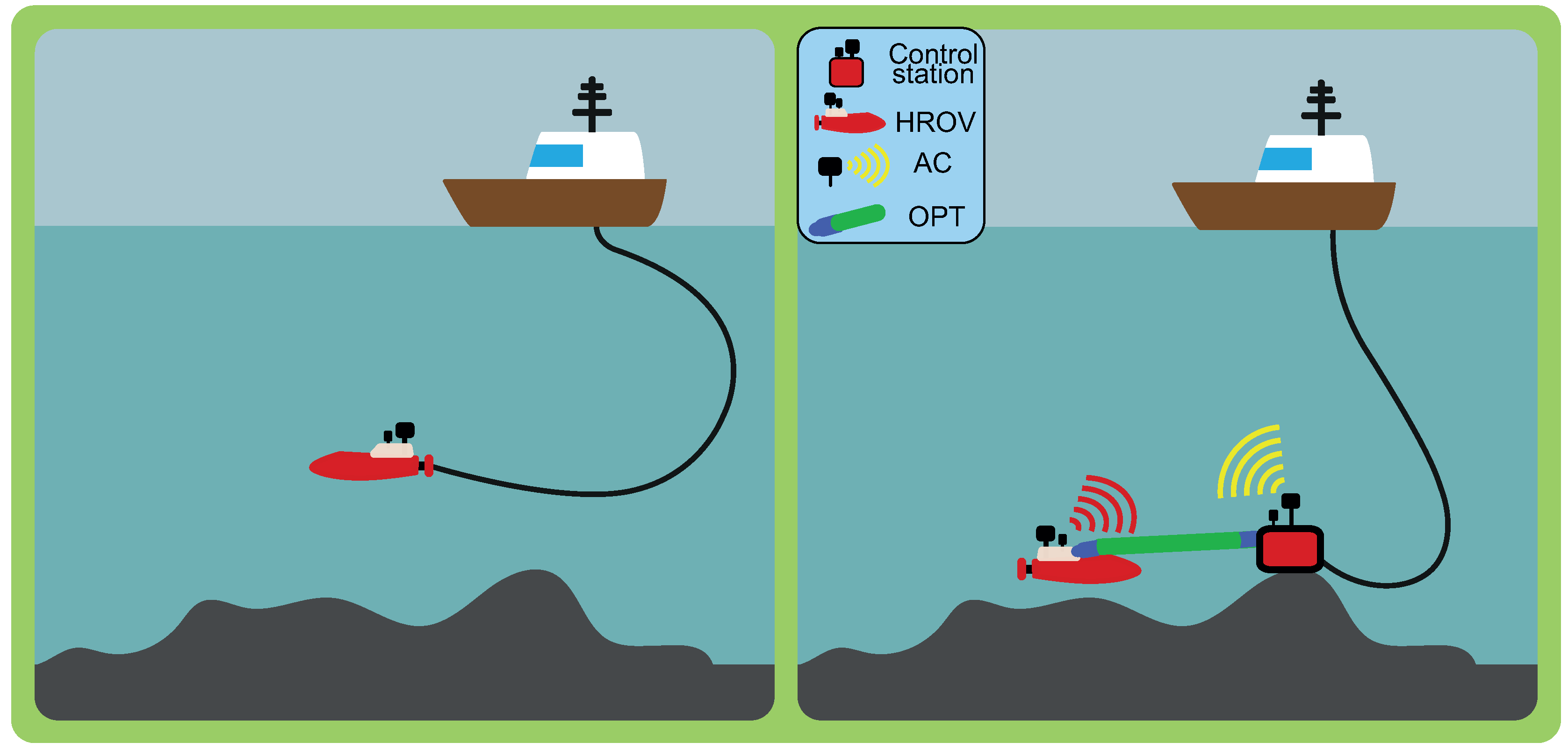
3.2. Short-Range Full-Capacity Wireless Mode

In this section, we describe the short-range full-capacity wireless mode (SRM) with its requirements in terms of supported types of traffic and their respective bit rates. According to the review presented in Section 2, the raw video produced by the BlueROV camera cannot be transmitted with any commercial off-the-shelf underwater communication system for a distance of more than 10 m; therefore, both a lower resolution and video coding should be employed. For example, from our test, a high-definition h264 video with resolution of 704 × 578 px at 25 fps can be sent with an average bit rate of 1.3 Mbps and a peak bit rate of 8 Mbps. With h264 compression, the ratio between maximum and average bit rates is higher than in raw videos due to the fact that, while the quasi static parts of the video can be compressed with high efficiency, the frames presenting fast motions cannot be compressed as much. This behavior is caused by the fact that the latter has low correlations between each other and, thus, they require more information to be represented in a smooth video. The video size can be reduced by lowering the frame rate or the video resolution or by forcing a different video bit rate. A solution to achieve a higher compression level without losing quality and resolution is to employ black and white videos: according to our tests, in the same environment, a grey-scale video with the same resolution would require 0.6 Mbps on average and a peak bit rate of 2.93 Mbps. Some ROVs, such as the Ageotec models Pegaso and Perseo [112], in addition to color video can also transmit black and white videos, which sometimes can provide better contrast than color streams. For this reason, in the SRM considered in this paper, we account for the transmission of both a high-quality black and white video and a high-quality color video with average bit rates of 0.6 Mbps and 1.3 Mbps, respectively.

Ideally, SRM should provide a QoS similar to the one obtained through the umbilical connector, where an operator can control the ROV lighting intensity, the cameras, and a gripper.

This mode to be supported requires traffic of at least 4.5 kbps from the control station to the ROV, and of approximately 2 Mbps from the ROV to the control station. Video and control delay should be kept as low as possible, and the video delay variance should be minimized. Indeed, it is possible to control a vehicle in real time even video monitoring with a constant delay of up to 1 s, but it is not possible to pilot a vehicle if the video has a variable delay ranging from 0.1 s to 0.5 s [113]. This variation on the delay is called jitter and can be analyzed through the packet delay variation (PDV) metric [114], computed as follows:

$$PDV=\sum _{i=1}^{N_v}\frac{\left|d\right(i+1)-d(i\left)\right|}{N_v},$$

(1)

where $N_v$ is the number of packets received for the considered video stream and $d\left(i\right)$ is the delay of the ith packet. If PDV is less than 3 ms [115], the video stream is smooth and can be used for real-time applications; otherwise, a de-jitter buffer [116] is needed to artificially introduce a buffering delay and to mitigate jitter: to obtain a zero-delay jitter video, the buffering delay has to be set equal to the maximum jitter expected by the video.

This mode can be supported up to a distance of a few tens of meters (depending on the optical range) by the simultaneous use of one optical modem for video streaming and joystic remote control and one acoustic modem with LBL to support ROV navigation and to send the monitoring status.

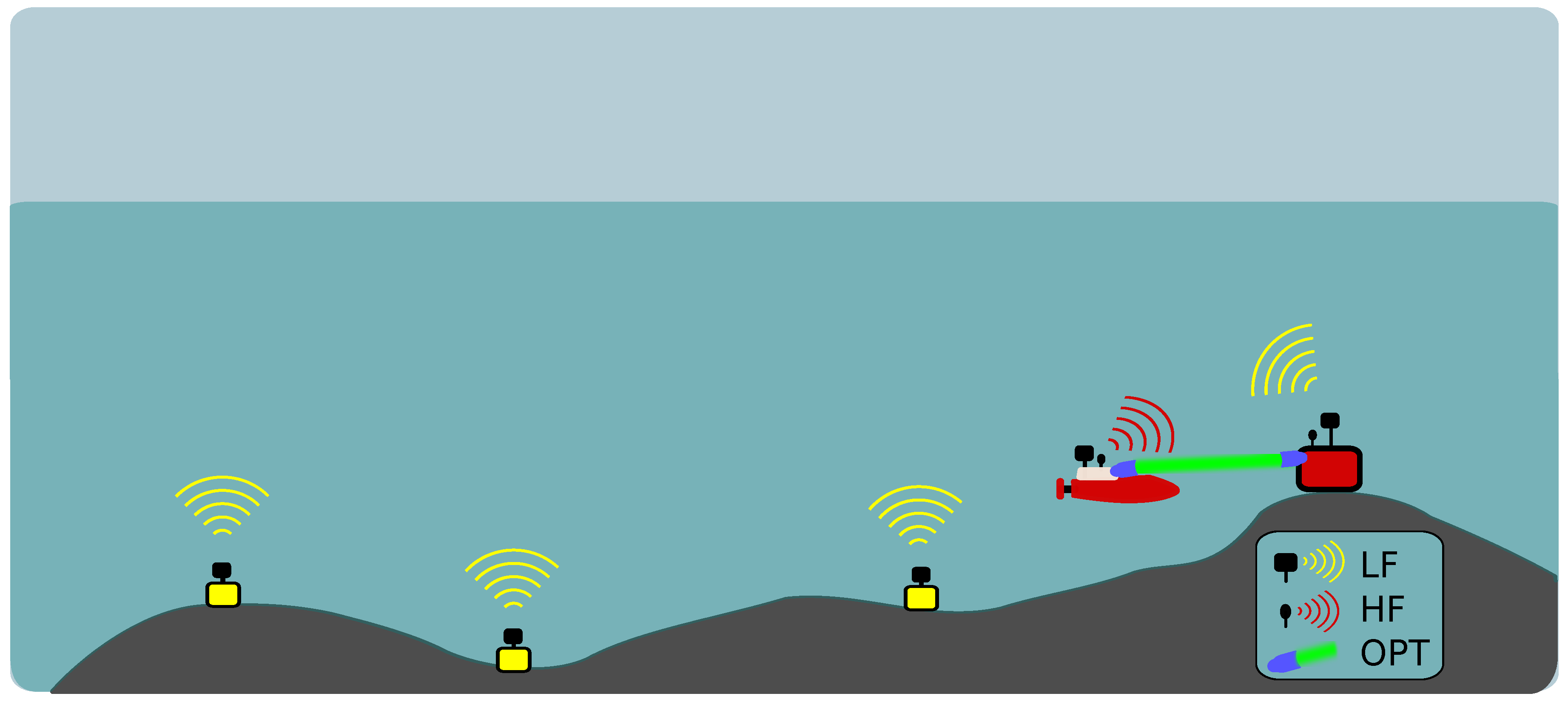
3.3. Mid-Range Low-Capacity Wireless Mode

In this mode, called mid-range low-capacity wireless mode (MRM), a real-time ROV remote control is no longer supported. Conversely from SRM, in MRM, position control is based on the transmission of way-points and not on a joystick-based trajectory control. A way-point-based remote control consists of sending not only the next position that the vehicle needs to reach but also the speed and rotation angles to the underwater vehicle, the latter used for setting the orientation of the vehicle while proceeding to the next position. The size of each component of position (x, y, and depth), speed (u, v, and w), and rotation angles (roll, pitch, and yaw) in a way-point packet is set equal to 4 bytes; therefore, together with a sequence number used as unique identifier of the way-point, the total size of a way-point packet is 40 bytes. In this mode, we assume that the minimum time lapse between two consecutive way-points is 2 s; thus, the maximum data rate generated by the control traffic is 160 bps.

The operator can observe the progress of the ongoing mission through a very low-quality non-real-time video feedback, streamed with a high-frequency acoustic modem. The video considered in this mode is a 200 × 96 px 5 fps VP9 video that requires an average bit rate of 13.7 kbps and a peak bit rate of 42 kbps. In [61], we managed to stream the same video through the EvoLogics S2CM HS acoustic modem: although the maximum bit rate is higher than the maximum throughput achievable by the modem in that tested conditions (20 kbps), the video was not blocked and the receiver was able to smoothly reproduce the video with few frame losses. Indeed, 14 frames, over a total of 645, were automatically discarded by the application used for streaming to avoid video jitter and additional delay. Due to the codec setup, stream visualization started 10 s after the beginning of transmission.

MRM can be supported by the simultaneous use of an HF acoustic modem for low-quality video stream plus the use of a long-range LBL acoustic modem for positioning, status monitoring, and sending the control messages up to a distance of a few hundred meters.

In this mode, although the gripper cannot be maneuvered due to the long latency of the video monitoring, still, it is possible for the ROV to take some high-definition pictures of some interesting areas. These pictures will be stored in the ROV and buffered until the system switches to SRM mode. MRM requires traffic up to 160 bps from the control station to the ROV (that includes way-point transmission and control of lights and cameras) and of at least 15 kbps from the ROV to the control station (very low-quality video and status monitoring).

3.4. Long-Range Minimum Control Wireless Mode

Also in the long-range minimum control wireless mode (LRM), real-time remote control is not supported. Similarly to MRM, the ROV position is controlled through the transmission of way-points but the low-quality video stream cannot be transmitted. This mode supports only position monitoring, LBL positioning, and the transmission of status updates. It makes use of an MF underwater multihop network to extend the control range up to 10 km from the control station. The operator in this case can only receive information about the ROV position and can transmit the next position that the vehicle needs to reach. In this mode, the average time between the transmission of 2 consecutive way-points is 60 s. Also in this mode, the gripper cannot be maneuvered due to the lack of video monitoring; still, it is possible for the ROV to take some high-definition pictures once it reaches a way-point. Moreover, an automatic identification system can decide to take some pictures in some areas where there might be damage to the underwater asset. These pictures will be stored in the ROV and buffered until the system switches to SRM mode. LRM requires traffic up to 50 bps from the control station to the ROV (that includes way-point transmission and control of lights and cameras) and at least 75 bps from the ROV to the control station to transmit periodic status information.

In both the MRM and LRM modes, the remote control requires a high level of autonomy for the underwater vehicle, that behaves more like an AUV than an ROV.

4. Scenario Description and Simulation Setup

The simulated scenario, depicted in Figure 4, included an underwater hybrid vehicle (HROV) able to operate both as an ROV and an AUV, a control station used to pilot the vehicle, and three relays used to extend the communication range between the vehicle and the control station. Both the control station and HROV were equipped with MF, HF acoustic, and optical modems, while the acoustic relays were equipped only with MF acoustic modems.

All simulations were performed with the DESERT Underwater [117] simulation framework. As presented in Section 2.4, we selected the BlueComm 200 optical modem, Subnero WNC, and the EvoLogics S2C HS communication devices; therefore, the simulations were configured according to the modem specifications, as will be presented later in this section and is summarized in

Table 5. Simulation parameters.

Parameter	Description
Optical attenuation coefficient	0.02–0.5 depending on the sea depth
Optical light noise conditions	Low light noise caused by external artificial sources.
Optical wavelength and data rate	470 nm, 4 Mbps
Optical MAC	TDMA (90% HROV, 10% control station)
Optical range	from 25 m to 75 m, depending on depth and alignment
MF data rate, carrier frequency, bandwidth	4 kbps, 24 kHz and 12 kHz
HF data rate, carrier frequency, bandwidth	30 kbps, 150 kHz and 60 kHz
HF MAC	CSMA
MF MAC	CSMA
General acoustic parameters	s = 1, w = 1 m/s, g = 1.75

.

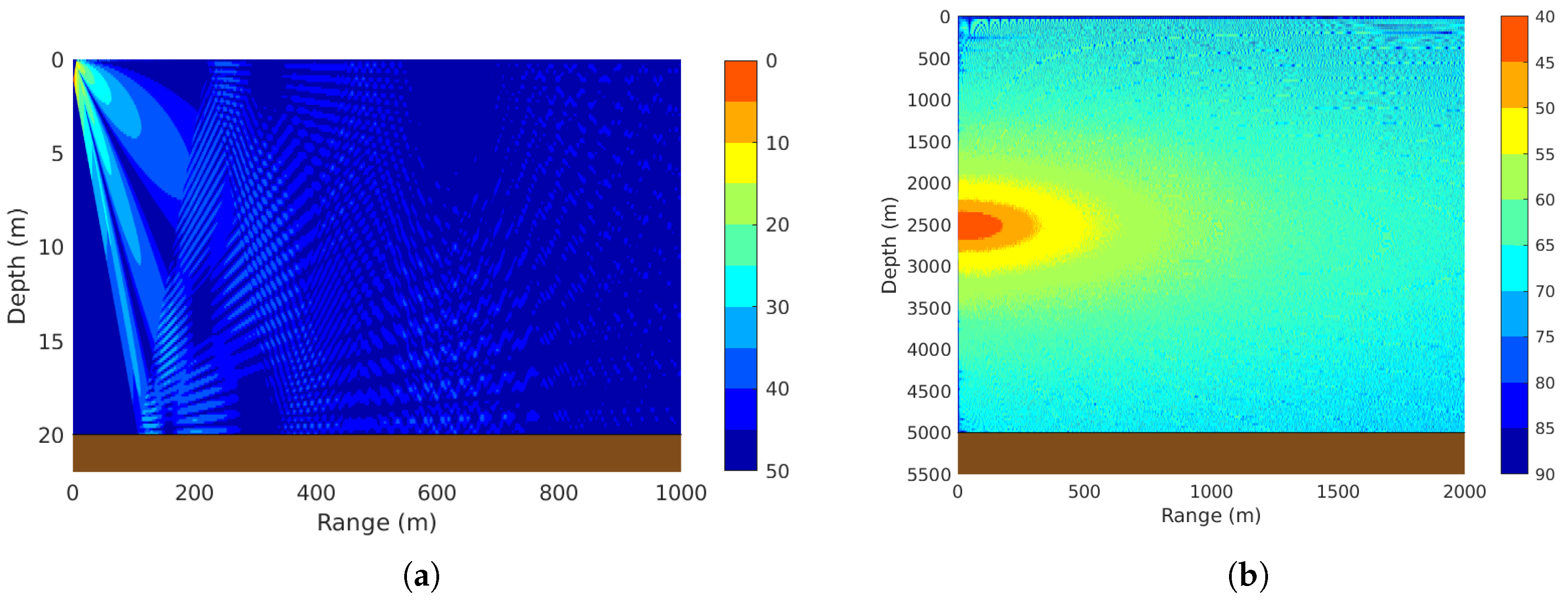
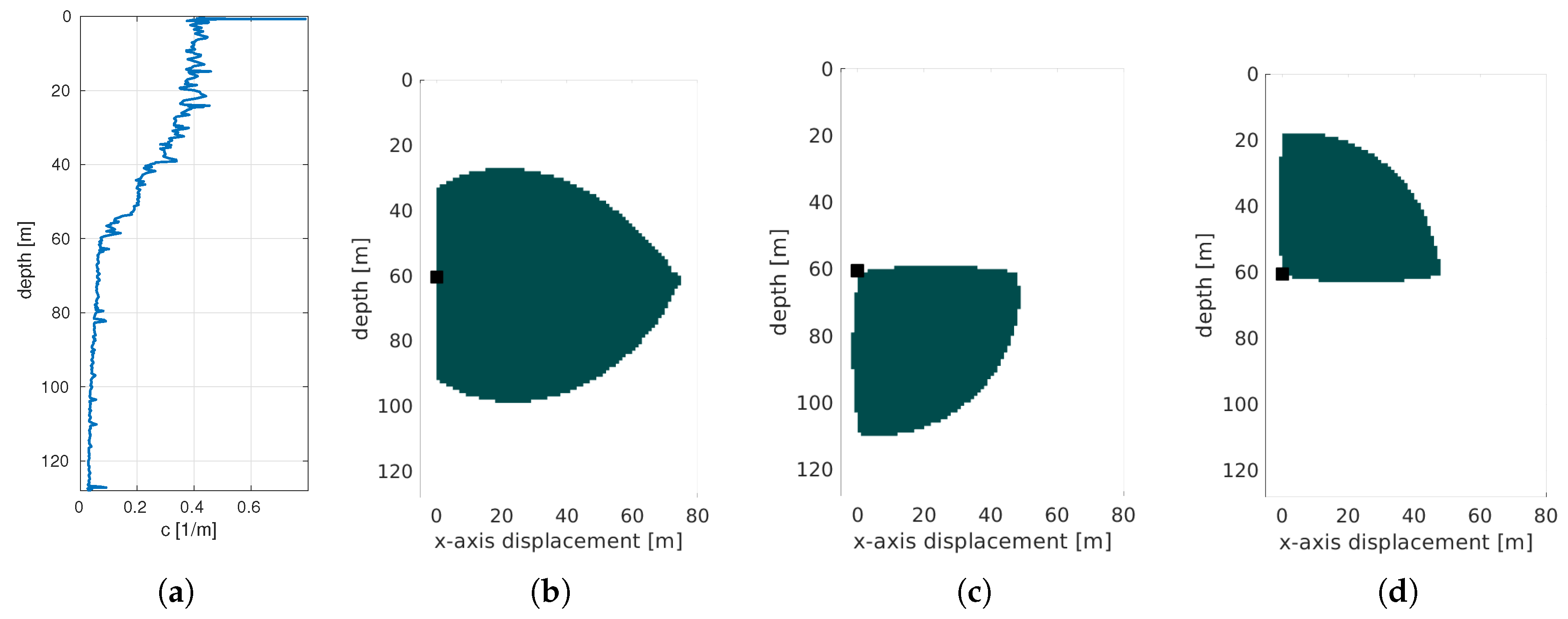
4.1. Optical Modem Simulator

The performance of the BlueComm 200 optical modem was mapped in the form of lookup tables (LUTs), as presented in [70], by considering a raw bit rate of 5 Mbps and the use of a forward error correction (FEC) mechanism with 80% efficiency (as declared from the manufacturer); hence, the actual data rate was 4 Mbps. Although the modem performs best in a deep, dark water environment, where oil and gas pipelines are typically deployed, in our simulations, we considered the performance of the modem when used in the presence of external lighting sources, such as the light needed for recording video streams, that introduced an important source of noise to the receiver, however, without saturating the photomultiplier. A similar effect was found when the BlueComm 200 optical modem was used during the night in shallow water, where it was observed that the moon, stars, and port lighting may reduce the maximum range of the optical communication to 1/3.

The maximum range of the optical communication also depends on how the attenuation coefficient changes along the water column: in this work, we used the values of the attenuation coefficient depicted in Figure 5a and measured during the ALOMEX’15 research cruise offshore the coast of Morocco (latitude 30${}^{\circ }$42.520’ N and longitude 10${}^{\circ }$18.680’ W). The ALOMEX’15 cruise was organized by the NATO STO Centre of Marine Research and Experimentation (CMRE), and its dataset was first presented in [18].

The last parameter that affects the optical range is the alignment between the transmitter and receiver. Indeed, the beam pattern of the BlueComm modem is hemispherical and not omnidirectional: this means that the maximum range and the receiving area also depend on the orientation of the two modems. In Figure 5, different cases are analyzed, keeping the position of the control station fixed at a depth of 60.5 m with the modem aligned to the x-axis and with three different setups of the modem installed in the underwater vehicle. First, in Figure 5b, we can observe the receiving area when the modem is installed in the back of the vehicle, that is assumed to be oriented along the x-axis, pointing directly to the modem in the control station. This leads to a symmetric receiving area and maximum range of 75 m; however, in this case, the vehicle can only be controlled by keeping fixed orientation, thus limiting vehicle maneuver. Two possible solutions can overcome this problem: one involves the installation of several modems on the same vehicle, obtaining omnidirectional coverage at the price of a more expensive deployment [24], and the other requires installation of the modem either in the top or in the bottom of the vehicle, hence orienting the modem along the z-axis. In Figure 5c,d we can observe how the receiving area and the maximum range are reduced to 50 m when the modem is installed in the top and in the bottom of the vehicle, respectively. Despite the shorter range, these solutions are not affected by the vehicle orientation in the x/y plane, thus providing good maneuverability. In this scenario, a larger coverage area is reached in Figure 5c because the attenuation coefficient decreases when increasing the sea depth (Figure 5a).

The BlueComm modems use blue wavelengths (470 nm) and a time division multiple access (TDMA) medium access control (MAC) layer that can split its time frame either into two equal time slots or into two time slots, where the former takes 10% of the TDMA frame and the latter takes 90% of the frame. Hence, we configured the optical MAC layer with this last setting, assigning 90% of the frame to the underwater vehicle for transmitting real-time video streams and 10% of the frame to the control station for the joystick position control.

4.2. Acoustic Modem Simulator

The Subnero WNC and the EvoLogics S2C HS acoustic modems were simulated by using two instances of the DESERT acoustic physical layer, called from here onwards MF PHY and HF PHY, respectively. Both PHYs were half duplex, i.e., they can either receive or transmit, and a mean-power interference model was employed. We implement the empirical underwater sound propagation and noise models described in [10], with a spreading coefficient g equal to 1.75 in the spreading loss component, shipping activity s equal to 1, and speed of wind w equal to 5 m/s. The speed of sound underwater was assumed to be constant and equal to 1500 m/s.

The MF PHY layer’s source level was 168 dB re $\mathsf{\mu }$Pa${}^2$ at 1 m: this value was used to match in the simulator the maximum range of 3.5 km declared from the modem manufacturer because, in the simulations, we did not consider transducer inefficiencies and multipath (the maximum source level of the actual modem was 185 dB re $\mathsf{\mu }$Pa${}^2$ at 1 m). The transmission rate was set to 4 kbps, the carrier frequency was 24 kHz, and the bandwidth was 12 kHz. Actually, a higher rate can be achieved, as a maximum bit rate of 15 kbps can be reached in good conditions: we used a lower bit rate because we considered horizontal transmissions, that often require adaptation of the bit rate to a lower value and the need for FEC and networking headers. In addition, in our design, the MF PHY was also used for LBL positioning, that usually comes at the cost of a lower communication rate, that motivates our bit rate choice.

The HF PHY layer’s source level was 156 dB re $\mathsf{\mu }$Pa${}^2$ at 1 m: also in this case, this value was used to match in the simulator a maximum range of 500 m (the maximum source level of the actual modem was 177 dB re $\mathsf{\mu }$Pa${}^2$ at 1 m). The net transmission rate was 30 kbps (a higher rate can be achieved, as a maximum bit rate of 62.5 kbps can be reached in good conditions, from which the bits needed for FEC and networking headers need to be removed), the carrier frequency was 150 kHz, and the bandwidth was 60 kHz.

Both PHYs used a carrier-sense MAC layer (CSMA).

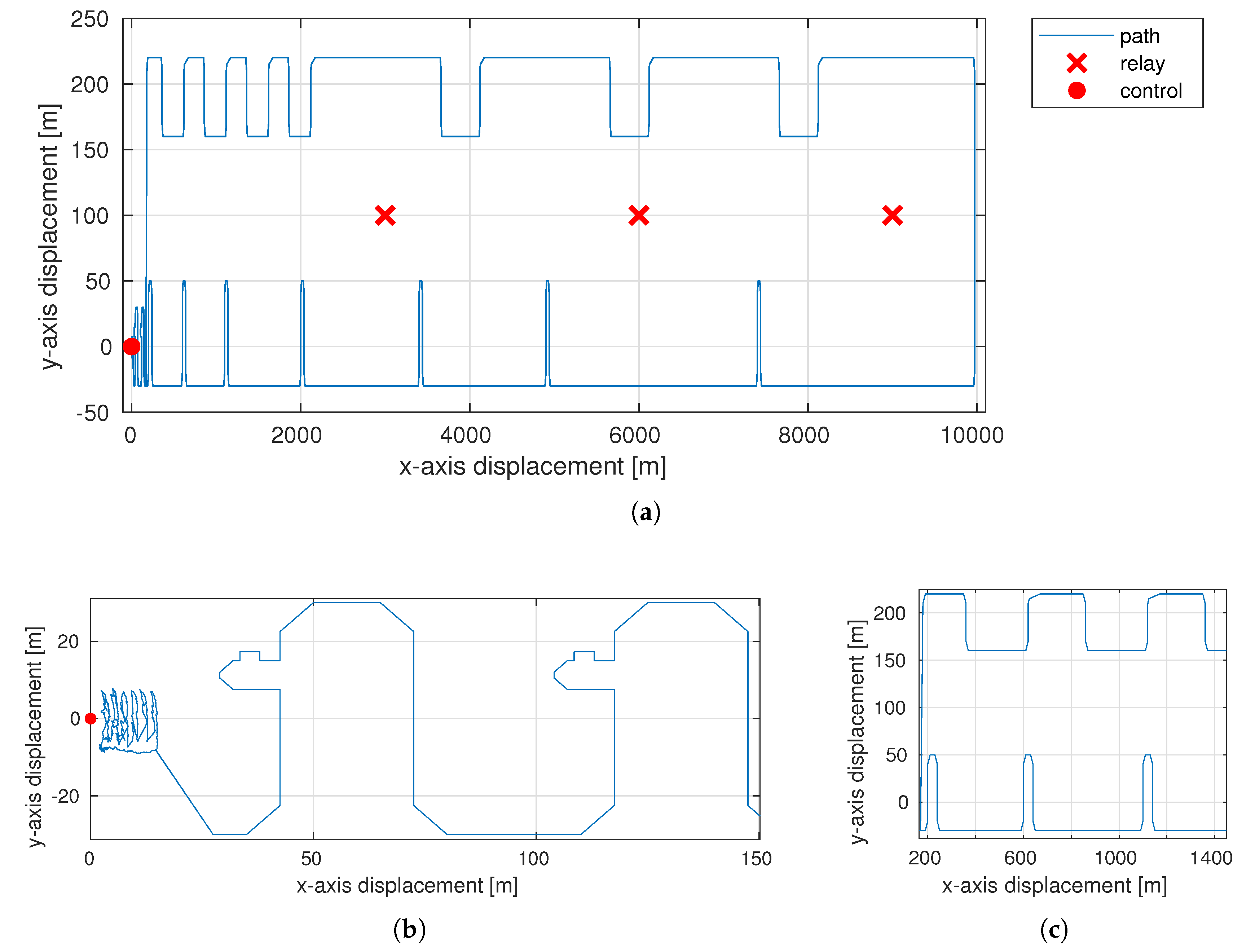
4.3. Nodes Deployment, Position Control, and Path

The application layer used to control the HROV position was first presented in [118], where the controller drove the underwater vehicle along the desired trajectory by sending absolute movement commands in the form of subsequent way-points to be covered and the speed that the HROV should use to reach that way-point. The y-x displacement of the resulting path when all way-points were reached is presented in Figure 6a, while the depth position changed between 9 m and 11 m. The three acoustic relays are represented with red crosses and were deployed 3000 m apart; the first relay was depicted 3000 m from the control station, that was deployed at the origin of the axes and represented with a red circle. Both the relays and the control station were deployed at a depth of 5 m.

To better visualize the path characteristics in different sections, we depict two zoomed-in parts in Figure 6b,c. The former presents the path in the proximity of the control station, and the latter presents the path from a distance of 200 m up to 1450 m far from the control station. The joystick control hwas simulated by sending several way-points close to each other. The section of the path depicted in Figure 6b from the coordinates (0, −10) and (20, 10) is the desired trajectory of the joystick control and was taken from the real motion of the CNR INM ROV described in [119]. During the dive performed in Biograd Na Moru [120,121], the ROV moved at an average speed of 0.2 m/s.

The remaining part of the path was controlled through way-point transmissions: the speed reaching a way-point varied from 0.5 m/s in zones where there were many details to inspect and precise maneuvers to be performed (e.g., the area depicted in Figure 6b) up to a speed of 1.5 m/s when the path was straight forward or did not require precise maneuvering (e.g., Figure 6c and the area that surround the relays in Figure 6a).

To this aim, two application layers were used at the control station:

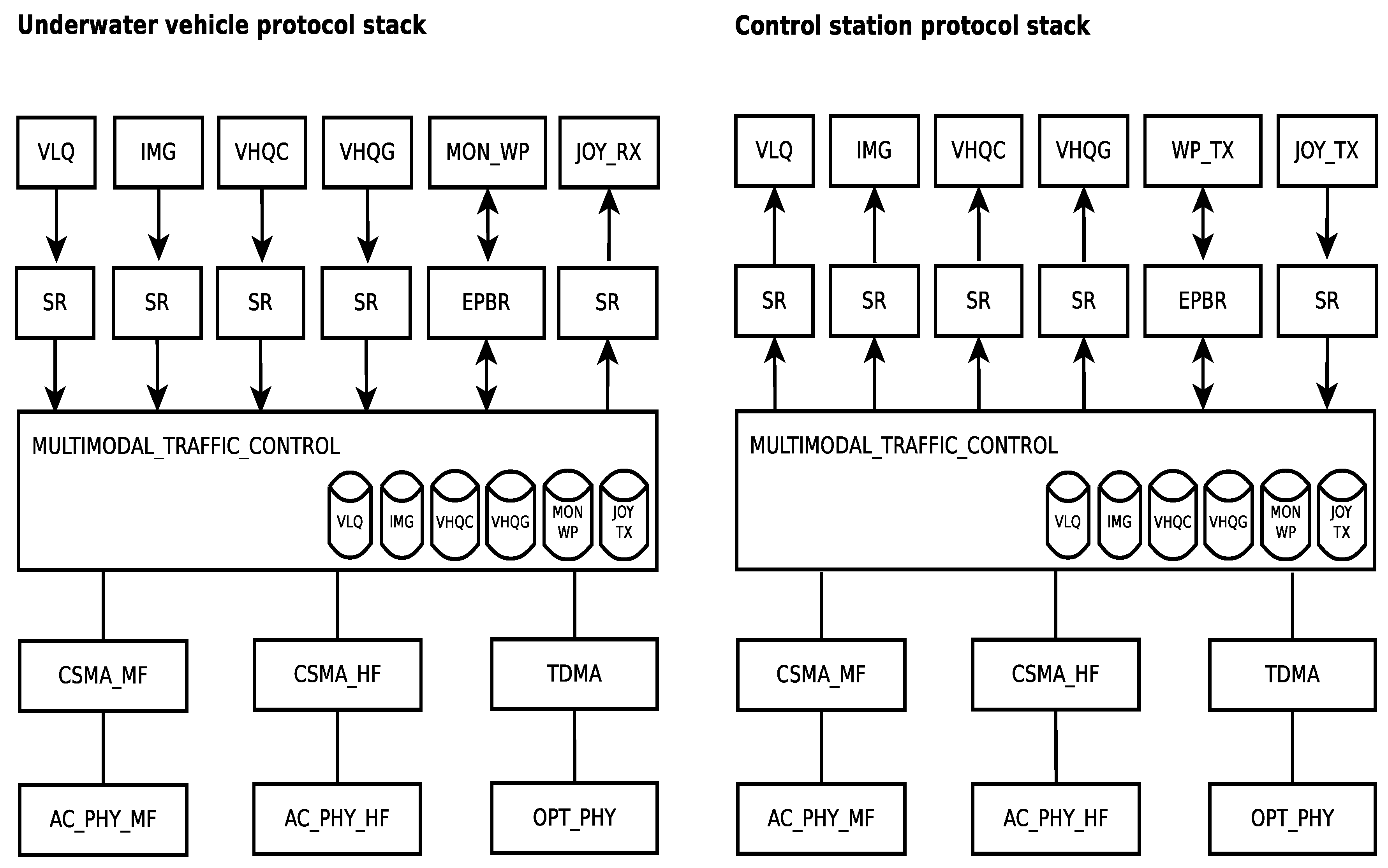
• JOY_TX, used to transmit the joystick control packet;
• WP_TX, used to transmit the way-point control packets.

4.4. Application Layers On-Board the Underwater Vehicle

Different application layers were used to transmit data from the HROV to the control station in order to simulate the data traffics required by each of the working modes described in Section 3. The application layers used in our simulations are listed in the following.

• MON_WP, a periodic application layer used to transmit monitoring packets with a size of 56 bytes every 6 seconds. This application layer also receives the way-point packets transmitted by the WP_TX application layer presented in Section 4.3 and sets the next way-point of the underwater vehicle accordingly.
• JOY_RX, an application layer used to receive the joystick position control by the JOY_TX application layer presented in Section 4.3 and to move the underwater vehicle accordingly.
• IMG, an application layer generating sporadic 4160 × 2336 pixel JPEG images with a size of 2.5 Megabytes, divided in packets with size 2 kilobytes. The images are generated on average every 1800 s according to a Poisson process.
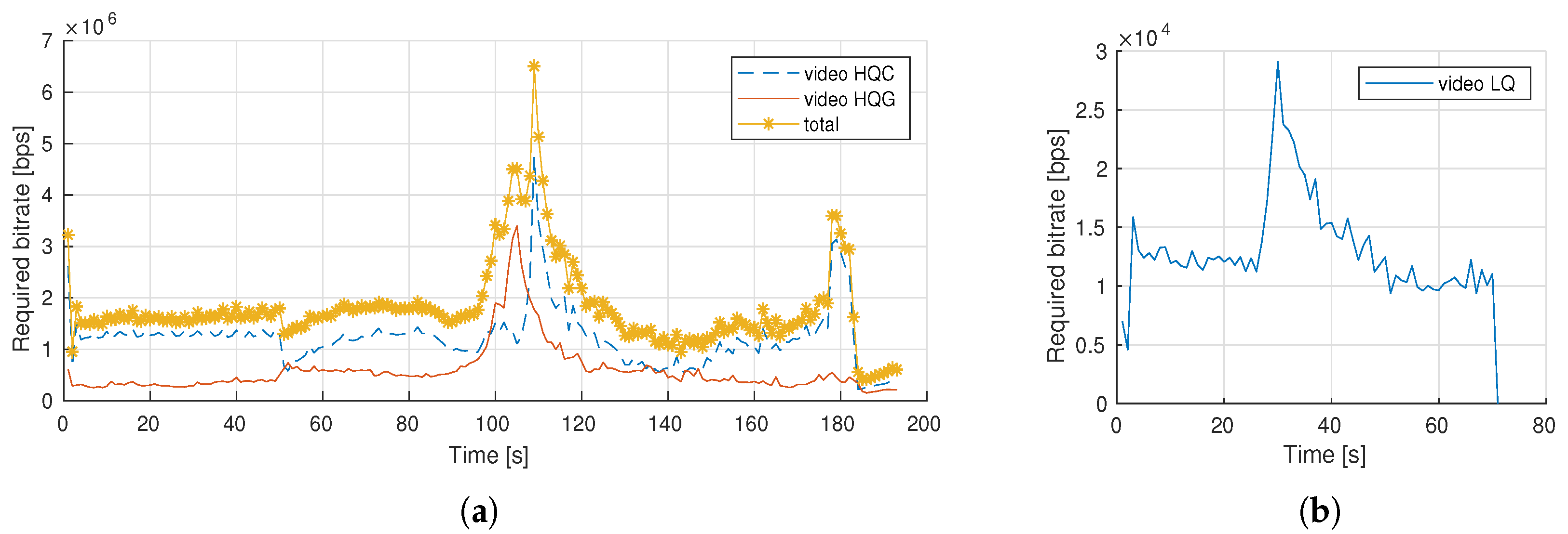
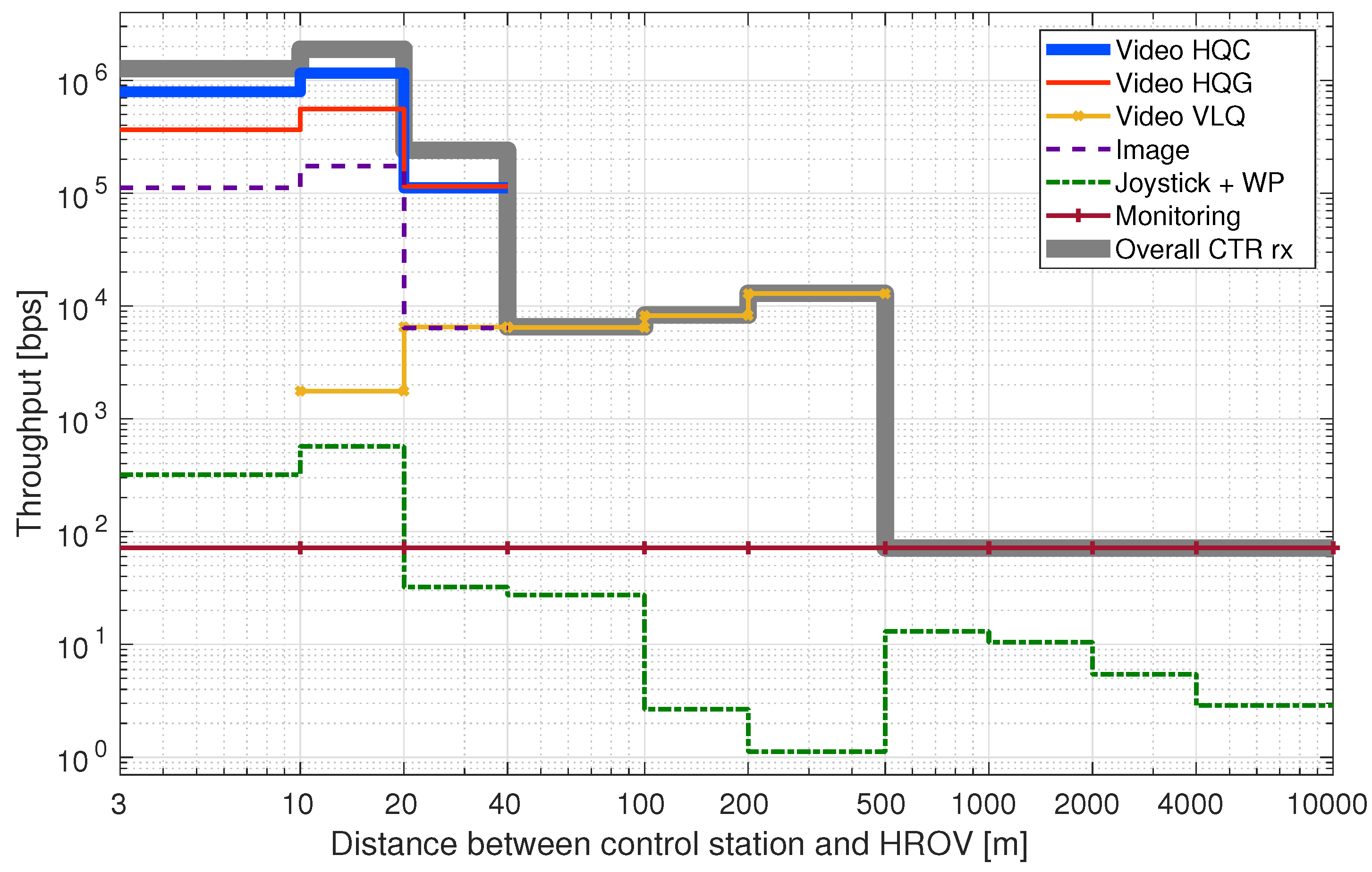
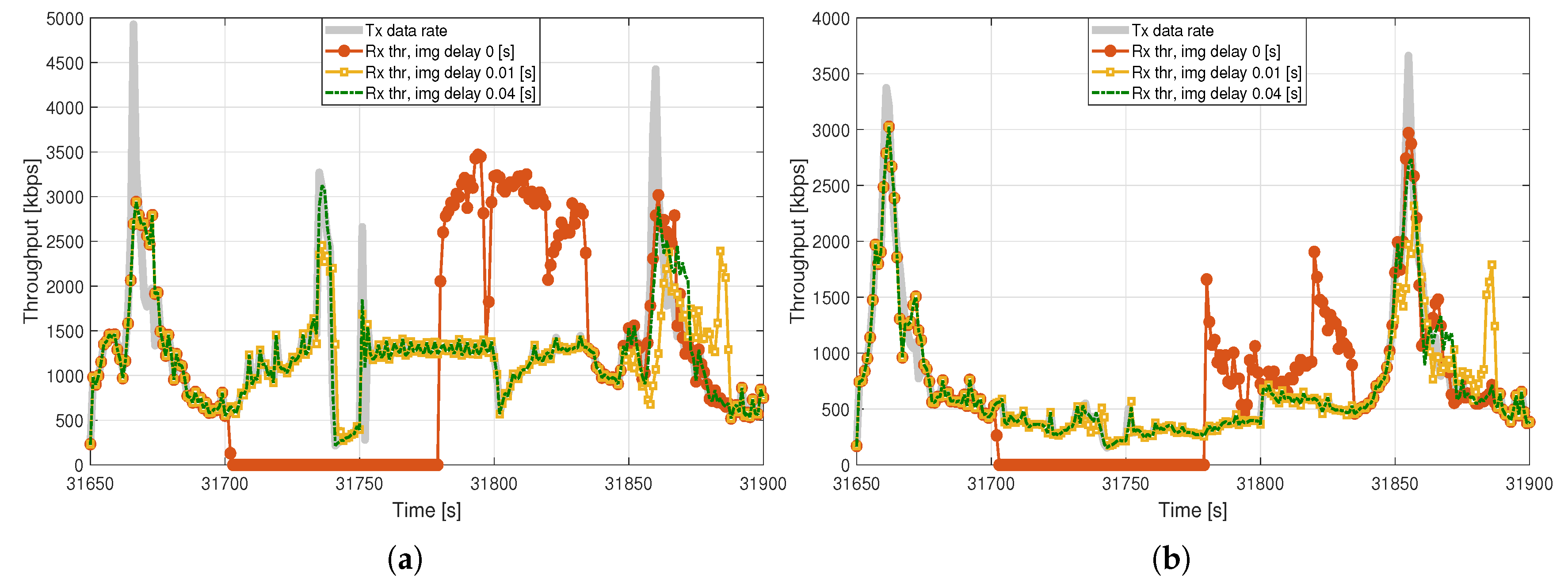
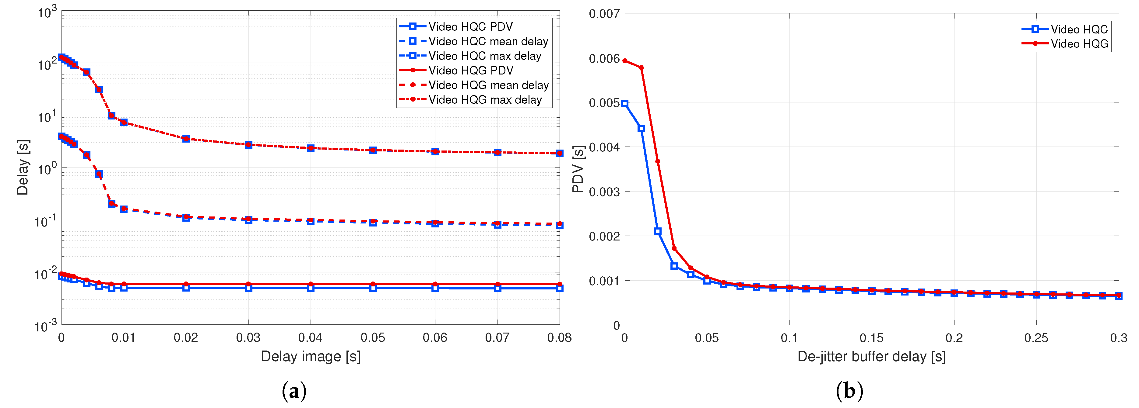
• VHQC, an application layer transmitting a high-quality real-time video stream, with an average bit rate of 1.3 Mbps. The packets were generated according to a 705 × 576 px at 25 fps video file with the instantaneous bit rate depicted in Figure 7a: in our simulation setup, each packet contained a frame, and the transmission period was 0.04 s.
• VHQG, an application layer transmitting a high-quality grey-scale real-time video stream, with average bit rate 0.6 Mbps. The packets were generated according to a 705 × 576 px at 25 fps video with the instantaneous bit rate depicted in Figure 7a: in our simulation setup, each packet contained a frame, and the transmission period was 0.04 s.
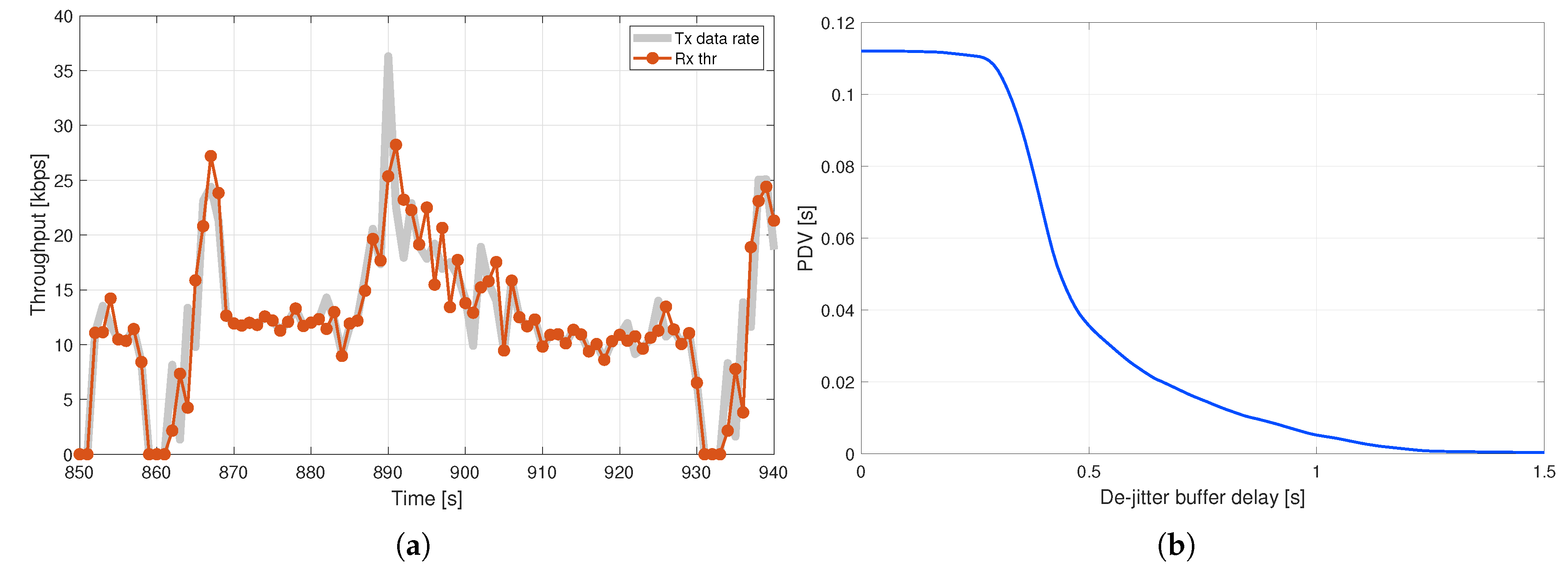
• VLQ, an application layer transmitting a very low-quality low-rate video, with average bit rate of 13.68 kbps. The packets were generated according to a 200 × 96 px at 5 fps video file with the instantaneous bit rate depicted in Figure 7b: in our simulation setup, each packet contained a frame, and the transmission period was 0.2 s.

4.5. Routing Protocols

All traffic types that cannot be transmitted through the multihop acoustic network due to the high throughput requirements, such as images, video streams, and joystick position control, were transmitted with the direct link from the control station and the HROV without the need for any routing layer: to simulate this in DESERT, we used a static routing (SR) layer where the address of the next hop and the destination were the same. Monitoring and way-point packets, instead, were transmitted through the underwater acoustic network. The packet routes in this case depended only on the HROV position; hence, for this types of traffic, we employed the Estimate-position based routing (EPBR) protocol, first presented in [15]. In this protocol, all static nodes (e.g., relays and control station) collected information about the position of the HROV and its speed and direction of movement from the packets received from the other nodes. The node topology and the position of relays and control station were assumed to be known by each node: in this way, both the relays and the control station could decide the best route of a packet for the HROV depending on their estimate of the HROV’s position while the HROV could decide whether to transmit a packet to a relay or to convey the packet directly to the control station observing its current position. Once a relay node received a packet sent by the HROV, it forwarded it to the control station via static routing. The HROV position estimate can be performed, for instance, through a Kalman filter or with the algorithm presented in [15].

4.6. Multimodal Layer

The level of flexibility to be supported by the multimodal system required the implementation of several features in the DESERT Underwater framework, such as the possibility of using different PHY technologies to convey traffics with different QoS requirements and a dynamic management of the network stack. For this reason, our transmission control module contains several queues, one for each type of traffic to be supported, that potentially presents a different behavior. Furthermore, the module is able to manage the queues dynamically to the correct combination of network protocols, MAC layer protocols, and PHY technologies.

For this reason, the multi_traffic_control layer presented in [122] was substantially extended to provide more functionalities, such as the possibility of setting the behavior of each queue used to buffer the outgoing data. For instance, a circular queue should be employed for video transmissions in order to avoid a long buffering time at the price of the loss of small segments of the video, while images need to be sent through a queue that is large enough to avoid discarding packets because even the loss of a small part of the image data will compromise the reception of the whole image. Moreover, this queuing management can be also used for traffic shaping. Specifically, while the default behavior of the multi_traffic_control layer lets the underlying physical layers transmit at their full capacity, this multimodal layer can also limit the transmission of a certain traffic type by forcing the packets stored in the corresponding transmission queue to be sent with a minimum inter-packet transmission time between each other, avoiding traffic without latency constraints saturating the physical layer. This is the case, for instance, of the image traffic: a whole image of size 2.5 Megabytes is indeed generated at one precise moment. If all packets required to carry this image are issued to be sent simultaneously, the optical physical layer will be completely devoted to the image transmission for almost 6 seconds, preventing all other traffic from being transmitted in the same time lapse. By setting an inter-packet transmission time bigger than 0 for the image traffic, instead the image packet transmissions can be limited, preventing, for instance, the video stream for being interrupted.

In the multi_traffic_control layer, each traffic type T had a list of lower layers through which it was possible to forward packets, either directly (in the case of long range links) or after channel probing (in the case of short range links). Specifically, in this work, all traffic packets intended to be transmitted via optical or short range acoustic required channel probing while packets sent through long-range acoustic were transmitted directly. The complete stack used in our simulations is depicted in Figure 8.

5. Simulation Results

In this section, we evaluate the designed system through simulations in order to verify whether the network can provide the QoS needed for HROV remote control. Network metrics such as throughput, packet delivery ratio, and packet delivery delay are analyzed for each data traffic. Moreover, also other metrics tailored to analyze specific application requirements are assessed, such as the packet delay variation of the video traffics and the root mean square error (RMSE) of the HROV path compared to the desired path. To analyze the impact of errors introduced by wireless communication on ROV control, we assume an optimal positioning system on-board the vehicle.

Figure 9 presents how the throughput of each traffic type varies with the distance between the receiver and the transmitter: the evidence is that the SRM can be supported up to a maximum distance of 40 m: from there onward, both HQ video streams and image traffics can no longer be transmitted. With the scenario considered for our simulations, this distance corresponds to the maximum range of the optical modem: we remark the importance to set into the simulator the expected conditions of the environment where the system has to be deployed because, considering waters with a different attenuation coefficient profile or different background light noise conditions, the maximum optical range can change drastically, from 100 m in deep dark waters down to 2 m when the modem is deployed 1 m below the sea surface during a sunny day.

MRM instead can be supported up to a distance of 500 m, when low quality video can no longer be sent. According to our simulation setup that neglected the multipath effect, this distance corresponds to the maximum distance of the HF modem: also in this case, we need to remark that, considering a different environment with more multipath or different noise sources, the range can be reduced (e.g., during a sea trial in 2019, we observed a maximum range of 200 m when the modem was deployed in very shallow water). From a distance of 500 m onward up to a distance of 10 km, only LRM can be supported, as only the basic monitoring traffic and the way-point position control packets can be transmitted through the MF acoustic network. The curves corresponding to the traffic types for which packets are generated according to predefined trace files (e.g., video streams, images, joystick, and way-point position control) present some variations in the bit rate between adjacent distance windows: this happens because the considered generation files are the same for all simulation runs, and when the HROV is at a distance between 10 m and 20 m, the transmitted video frames are larger than the video frames transmitted when the HROV is at a distance between 3 m and 10 m from the control station.

5.1. Joystick and Way-Point Position Control

Joystick (JOY_TX) and way-point (WP_TX) packets are sent from the control station to the HROV to control the HROV trajectory. For these applications, packet loss caused by a combination of channel error, deafness, and interference may result in some error on the trajectory performed by the HROV: while this is not the case for the JOY_TX packets sent in short range with a broadband optical link that has a negligible packet error rate (PER) when in range, this effect can be observed in the transmission of the WP_TX packets sent through the acoustic network, as their PER is 5.5%. In order to measure the trajectory error, we computed the RMSE of the path followed by the HROV with respect to the original path. Specifically, in Figure 10, we report the value of the RMSE for different positions of the HROV, observing that the RMSE linearly increases with distance as long as the distance between the HROV and the control station is less than 2.5 km, for which the RMSE is 3.5 m. Surprisingly, for longer distances, the trend changes drastically, as the RMSE no longer increases with distance. Specifically, in correspondence to the position of the first acoustic relay, we observe a peak of the RMSE that increases up to 14 m: from there onward, the RMSE oscillates between a value of 2 m and a value of 7.5 m when the HROV is 10 km from the control station. The reason for this behavior is the fact that, with the MAC layer being used for WP_TX contention, we cannot predict when a packet is lost due to deafness or collisions. Still, from our simulations, it results that, even in the worst case, the RMSE is always smaller than 20 m for all trajectorues. Moreover, for distances up to 500 m where the HROV path is quite detailed (Figure 6b), the RMSE is always less than 1 m, while in the area controlled through joystick (up to a distance of 30 m from the control station), the RMSE is always less than 0.2 m. These results have been obtained by transmitting subsequent way-points, sending a new position as soon as the HROV should have reached the previous way-point in case of no packet loss without employing any additional guard time between the transmission of subsequent way-points. Nevertheless, the RMSE is always less than 0.6% of the distance between the HROV and the control station, that is in the order of magnitude of the existing tracking system accuracy. Still, if a smaller RMSE is required, a guard time between subsequent way-points can be employed to allow packets retransmissions [118], at the price of a longer mission duration.

5.2. Video and Images: Traffic Shaping and Video De-Jittering Buffer

Packet delay variation (PDV) strongly affects multimedia streams, causing clumping and dispersion. A large PDV is caused by both the fact that a video stream is composed of frames with different size and the presence of other types of traffic injected into the network. In our case, on the one hand, the acoustic HF modem is required to transmit a VLQ video that requires a variable bit rate and, on the other hand, the optical channel is required to service 2 video streams and image transmissions at the same time. Figure 11a presents the difference between the transmitted (grey line) and the received (red line) instantaneous video bit rate of the VLQ stream: thanks to the fact that the acoustic HF channel is completely dedicated to the transmission of the VLQ stream, the two bit rates are quite similar, with the exclusion of the maximum bit rate peak, that is higher than the maximum throughput achievable with acoustic HF. The average delay of the VLQ stream is 514 ms, while the PDV of this video stream is equal to 112 ms, two orders of magnitude higher than the maximum PDV required for a smooth video stream, that is equal to 3 ms [115]. To mitigate the PDV effect, a de-jittering buffer can be employed at the receiver: indeed, as long as the bandwidth can support the stream and the buffer size is sufficient, buffering only causes a detectable delay before the start of media playback. Specifically, a PDV less than 3 ms can be obtained with a de-jitter buffer that introduces a delay of 1.1 s (Figure 11b).

Figure 12a,b presents the difference between the transmitted (grey line) and the received (red line) instantaneous video bit rate of the VHQC and VHQG streams, respectively: it can be observed that, from 31,702 to 31,782 s, there is a drop in the received bit rate: this happens due to the fact that some acquired images are in the process of being transmitted, saturating all the bandwidth of the optical modem. This undesired effect can be mitigated by using traffic shaping, e.g., by limiting the image packets transmission in time, setting a minimum transmission delay between subsequent image traffic, called image delay from here onward, larger than zero. The expectation of performance gain introduced by traffic shaping is confirmed by both the yellow and the green lines, where the image delays have been set equal to 10 ms and 40 ms, respectively. Moreover, in the latter case, the received video bit rate is quite similar to the transmitted bit rate, with the exclusion of the bit rate peaks that are higher than the maximum throughput achievable with the optical modem. Figure 13a shows how the introduction of traffic shaping also reduces the average and the maximum video delay as well as the PDV of both VHQC and VHQG. Indeed, while without traffic shaping the average video delay is 3 s and the PDV is 10 ms, with an image delay of 40 ms the average video delay is less than 100 ms and the PDV is 5 ms for VHQC and 6 ms for VHQG. In order to further lower the PDV, a de-jitter buffer can be employed (Figure 13a): to reach the target PDV of 3 ms, a de-jitter buffer that adds a minimum delay of 30 ms can be employed.

6. Conclusions

In this paper, we designed and evaluated a wireless remote control for underwater vehicles in light of the capabilities offered by current optical, RF, and acoustic modem technologies. For each technology, we focused on the available modems that report performance figures measured in the presence of realistic operational conditions, including turbidity, sunlight noise, channel geometry, and the noise cause by the vehicle’s propellers. We then identified three operational modes based on the quality of service needed to pilot an HROV with incremental level of autonomy by defining all traffic types that each mode should be able to transmit through the underwater channel. Specifically, the vehicle can be piloted as an inspection-class ROV up to a range of few tens of meters, depending on the working conditions, while it can perform semiautonomous missions with a high control quality up to a range of few hundred of meters and quasi-autonomous missions up to a distance of 10 km. Actual samples of real streams have been used both to estimate the throughput that each mode needs to support and to generate the data packets transmitted in our simulation.

We designed and implemented in the DESERT Underwater framework a multimodal communication layer able to support different QoSs for each traffic type to be transmitted, with the use of dedicated queues that can also be used for traffic shaping by setting the minimum delay between subsequent packets of the same traffic type. Via simulations, we were able to tune this delay of not-time-stringent burst traffics in order to prioritize all traffics with real-time requirements. To this aim, we also inspect the effects caused by a de-jitter buffer able to limit packet delay variation at the cost of a higher delivery delay. We analyzed the root mean square error of the path followed by the HROV compared to the desired path that resulted in always being less than 0.6% of the distance between the HROV and the control station. Nevertheless, the accuracy of the actual trajectory relative to the desired one can be improved by increasing the guard time between subsequent commands, at the price of a longer mission and, therefore, the need for a higher battery capacity.

Future works will focus on realizing a proof-of-concept prototype (PoC) of the system and on evaluating it through a field test.

References

1. Capocci, R.; Dooly, G.; Omerdic, E.; Coleman, J.; Newe, T.; Toal, D. Inspection-Class Remotely Operated Vehicles-A Review. J. Mar. Sci. Eng. 2017, 5, 13. [Google Scholar] [CrossRef]
2. Kraken Seavision. Available online: https://krakenrobotics.com/products/seavision/ (accessed on 21 September 2020).
3. Campagnaro, F.; Francescon, R.; Casari, P.; Diamant, R.; Zorzi, M. Multimodal Underwater Networks: Recent Advances and a Look Ahead. In Proceedings of International Conference on Underwater Networks & Systems; Association for Computing Machinery, New York, NY, USA, 2017. [Google Scholar]
4. Wireless For Subsea Seatooth. Available online: https://www.wfs-tech.com/product/seatooth/ (accessed on 21 September 2020).
5. Ardelt, G.; Mackenberg, M.; Markmann, J.; Esemann, T.; Hellbruck, H. A Flexible and Modular Platform for Development of Short-Range Underwater Communication. In Proceedings of the 11th ACM International Conference on Underwater Networks & Systems, Shanghai, China, 24–26 October 2016. [Google Scholar]
6. Inacio, S.I.; Pereira, M.R.; Santos, H.M.; Pessoa, L.M.; Teixeira, F.B.; Lopes, M.J.; Aboderin, O.; Salgado, H.M. Dipole Antenna for Underwater Radio Communications. In Proceedings of the 2016 IEEE Third Underwater Communications and Networking Conference (UComms), Lerici, Italy, 30 August–1 September 2016. [Google Scholar]
7. Sonardyne BlueComm Optical Modem. Available online: https://www.sonardyne.com/product-category/wireless-communications/very-high-data-rate/ (accessed on 21 September 2020).
8. Caiti, A.; Ciaramella, E.; Conte, G.; Cossu, G.; Costa, D.; Grechi, S.; Nuti, R.; Scaradozzi, D.; Sturniolo, A. OptoCOMM: Introducing a new optical underwater wireless communication modem. In Proceedings of the 2016 IEEE Third Underwater Communications and Networking Conference (UComms), Lerici, Italy, 30 August–1 September 2016. [Google Scholar]
9. AQUAmodem Op1 Optical Modem Page. Available online: http://www.aquatecgroup.com/aquamodem/aquamodem-op1 (accessed on 21 September 2020).
10. Stojanovic, M. On the relationship between capacity and distance in an underwater acoustic communication channel. ACM Mob. Comput. Commun. Rev. 2007, 11, 34–43. [Google Scholar] [CrossRef]
11. Develogic Subsea Systems. Available online: http://www.develogic.de/ (accessed on 21 September 2020).
12. Freitag, L.; Grund, M.; Singh, S.; Partan, J.; Koski, P.; Ball, K. The WHOI Micro-Modem: An Acoustic Communications and Navigation System for Multiple Platforms. 2005. Available online: http://www.whoi.edu (accessed on 21 September 2020).
13. Bowen, A.D.; Jakuba, M.V.; Farr, N.E.; Ware, J.; Taylor, C.; Gomez-Ibanez, D.; Machado, C.R.; Pontbriand, C. An Un-Tethered ROV for Routine Access and Intervention in the Deep Sea. In Proceedings of the 2013 Oceans-San Diego, San Diego, CA, USA, 21–25 October 2013. [Google Scholar]
14. Campagnaro, F.; Guerra, F.; Favaro, F.; Calzado, V.S.; Forero, P.; Zorzi, M.; Casari, P. Simulation of a Multimodal Wireless Remote Control System for Underwater Vehicles. In Proceedings of the 10th International Conference on Underwater Networks & Systems, Washington, DC, USA, 22–24 October 2015. [Google Scholar]
15. Signori, A.; Campagnaro, F.; Zorzi, M. Multi-Hop Range Extension of a Wireless Remote Control for Underwater Vehicles. In Proceedings of the 2018 OCEANS-MTS/IEEE Kobe Techno-Oceans (OTO), Kobe, Japan, 28–31 May 2018. [Google Scholar]
16. Tena, I. Navigating Underwater Autonomy. ROV Planet Mag. 2020, 1, 8037–8051. Available online: https://issuu.com/rovplanet/docs/rovplanet_magazine_022__web_ (accessed on 21 September 2020).
17. Maslin, E. Winning the subsea space race. IET Eng. Technol. 2020, 15, 8037–8051. [Google Scholar]
18. Diamant, R.; Campagnaro, F.; De Grazia, M.D.F.; Casari, P.; Testolin, A.; Calzado, V.S.; Zorzi, M. On the Relationship between the Underwater Acoustic and Optical Channels. IEEE Trans. Wirel. Commun. 2017, 16, 8037–8051. [Google Scholar] [CrossRef]
19. Sani, M.I.; Siregar, S.; Kurniawan, A.P.; Irwan, M.A. FIToplankton: Wireless Controlled Remotely-operated Underwater Vehicle (ROV) for Shallow Water Exploration. Int. J. Electr. Comput. Eng. (IJECE) 2018, 8, 3325–3332. [Google Scholar] [CrossRef] [Green Version]
20. Cruz, N.A.; Ferreira, B.M.; Kebkal, O.; Matos, A.C.; Petrioli, C.; Petroccia, R.; Spaccini, D. Investigation of Underwater Acoustic Networking Enabling the Cooperative Operation of Multiple Heterogeneous Vehicles. Mar. Technol. Soc. J. 2013, 47, 43–58. [Google Scholar] [CrossRef] [Green Version]
21. Centelles, D.; Soriano, A.; Marin, R.; Sanz, P.J. Wireless HROV Control with Compressed Visual Feedback Using Acoustic and RF Links. J. Intell. Robot. Syst. 2020, 99, 713–728. [Google Scholar] [CrossRef] [Green Version]
22. BlueROV2. Available online: https://bluerobotics.com/store/rov/bluerov2/ (accessed on 21 September 2020).
23. Ali, M.F.; Perera, T.D.P.; Morapitiya, S.S.; Jayakody, D.N.K.; Panic, S.; Garg, S. A Hybrid RF/FSO and Underwater VLC Cooperative Relay Communication System. In Proceedings of the 14th International Forum on Strategic Technology (IFOST-2019), Tomsk, Russia, 14–17 October 2019. [Google Scholar]
24. EXRAY. Available online: https://www.hydromea.com/exray-wireless-underwater-drone/ (accessed on 21 September 2020).
25. LUMA. Available online: https://www.hydromea.com/underwater-wireless-communication/ (accessed on 21 September 2020).
26. Miller, N. An Underwater Communication System. IEEE IRE Trans. Commun. Syst. 1959, 7, 249–251. [Google Scholar] [CrossRef]
27. Porter, M. Bellhop Code. Available online: http://oalib.hlsresearch.com/Rays/index.html (accessed on 21 September 2020).
28. Teledyne-Benthos Acoustic Modems. Available online: http://www.teledynemarine.com/acoustic-modems/ (accessed on 21 September 2020).
29. Underwater Acoustic Modems. Available online: https://evologics.de/acoustic-modems (accessed on 21 September 2020).
30. AQUASENT Acoustic Modems. Available online: http://www.aquasent.com/acoustic-modems/ (accessed on 21 September 2020).
31. LinkQuest Underwater Acoustic Modems. Available online: http://www.link-quest.com/html/models1.htm (accessed on 21 September 2020).
32. Communication Design. Available online: http://www.aquatecgroup.com/19-solutions/107-communication-design (accessed on 21 September 2020).
33. MATS 3G multi-modulation acoustic telemetry system. Available online: http://www.sercel.com/products/Pages/mats3g.aspx (accessed on 21 September 2020).
34. Modems for Underwater Communication. Available online: https://www.kongsberg.com/maritime/products/Acoustics-Positioning-and-Communication/modems/ (accessed on 21 September 2020).
35. Freitag, L.; Ball, K.; Partan, J.; Koski, P.; Singh, S. Long range acoustic communications and navigation in the Arctic. In Proceedings of the OCEANS 2015-MTS/IEEE Washington, Washington DC, USA, 19–22 October 2015. [Google Scholar]
36. Popoto Modem. Available online: http://popotomodem.com/ (accessed on 21 September 2020).
37. Cario, G.; Casavola, A.; Lupia, M.; Rosace, C. SeaModem: A Low-Cost Underwater Acoustic Modem for Shallow Water Communication. In Proceedings of the OCEANS 2015-Genova, Genova, Italy, 19–22 October 2015. [Google Scholar]
38. Sonardyne. Underwater Acoustic Modem 6. Available online: https://www.sonardyne.com/product/underwater-acoustic-modems/ (accessed on 21 September 2020).
39. Low Cost Underwater Acoustic modem for Makers of Underwater Things and OEMs! Available online: https://dspcommgen2.com/news-flash-low-cost-acoustic-modems-and-transducers-available-for-sale-now/ (accessed on 21 September 2020).
40. Subnero. Available online: https://subnero.com/ (accessed on 21 September 2020).
41. SeaTrac Technology. Available online: https://www.blueprintsubsea.com/seatrac/technology.php (accessed on 21 September 2020).
42. Shimura, T.; Kida, Y.; Deguchi, M. High-rate acoustic communication at the data rate of 69 kbps over the range of 3600 m developed for vertical uplink communication. In Proceedings of the OCEANS 2019-Marseille, Marseille, France, 17–20 June 2019. [Google Scholar]
43. Binnerts, B.; Mulders, I.; Blom, K.; Colin, M.; Dol, H. Development and demonstration of a live data streaming capability using an underwater acoustic communication link. In Proceedings of the 2018 OCEANS-MTS/IEEE Kobe Techno-Oceans (OTO), Kobe, Japan, 28–31 May 2018. [Google Scholar]
44. Otnes, R.; Locke, J.; Komulainen, A.; Blouin, S.; Clark, D.; Austad, H.; Eastwood, J. Dflood network protocol over commercial modems. In Proceedings of the 2018 Fourth Underwater Communications and Networking Conference (UComms), Lerici, Italy, 28–30 August 2018. [Google Scholar]
45. Dol, H.; Colin, M.; van Walree, P.; Otnes, R. Field experiments with a dual-frequency-band underwater acoustic network. In Proceedings of the 2018 Fourth Underwater Communications and Networking Conference (UComms), Lerici, Italy, 28–30 August 2018. [Google Scholar]
46. Underwater Communication Systems. Available online: https://www.wartsila.com/marine/build/sonars-naval-acoustics/underwater-communication-systems (accessed on 21 September 2020).
47. L3HARRIS. Available online: https://www2.l3t.com/oceania/ (accessed on 21 September 2020).
48. Tapparello, C.; Casari, P.; Toso, G.; Calabrese, I.; Otnes, R.; van Walree, P.; Goetz, M.; Nissen, I.; Zorzi, M. Performance Evaluation of Forwarding Protocols for the RACUN Network. In Proceedings of the Eighth ACM International Conference on Underwater Networks and Systems, Kaohsiung, Taiwan, 11–13 November 2013. [Google Scholar]
49. Potter, J.; Alves, J.; Green, D.; Zappa, G.; Nissen, I.; McCoy, K. The JANUS underwater communications standard. In Proceedings of the 2014 Underwater Communications and Networking (UComms), Lerici, Italy, 3–5 September 2014. [Google Scholar]
50. Sherlock, B.; Neasham, J.A.; Tsimenidis, C.C. Implementation of a spread-spectrum acoustic modem on an android mobile device. In Proceedings of the OCEANS 2017-Aberdeen, Aberdeen, UK, 19–22 June 2017. [Google Scholar]
51. Morozs, N.; Mitchell, P.D.; Zakharov, Y.; Mourya, R.; Petillot, Y.R.; Gibney, T.; Dragone, M.; Sherlock, B.; Neasham, J.A.; Tsimenidis, C.C.; et al. Robust TDA-MAC for practical underwater sensor network deployment: Lessons from USMART sea trials. In Proceedings of the Thirteenth ACM International Conference on Underwater Networks & Systems, Shenzhen, China, 3–5 December 2018. [Google Scholar]
52. Benson, B.; Li, Y.; Faunce, B.; Domond, K.; Kimball, D.; Schurgers, C.; Kastner, R. Design of a Low-Cost Underwater Acoustic Modem. IEEE Embed. Syst. Lett. 2010, 2, 58–61. [Google Scholar] [CrossRef] [Green Version]
53. Tritech Micron Modem—Acoustic Modem. Available online: https://www.tritech.co.uk/product/micron-data-modem (accessed on 21 September 2020).
54. Desert Star Systems. SAM-1 Technical Reference Manual. Available online: https://desertstarsystems.nyc3.digitaloceanspaces.com/Manuals/SAM-1TechnicalReferenceManual.pdf (accessed on 21 September 2020).
55. DiveNET: Sealink. Available online: https://www.divenetgps.com/sealink (accessed on 21 September 2020).
56. Renner, B.C.; Heitmann, J.; Steinmetz, F. ahoi: Inexpensive, Low-power Communication and Localization for Underwater Sensor Networks and AUVs. ACM Trans. Sens. Networks 2020, 16, 1–46. [Google Scholar] [CrossRef] [Green Version]
57. Water Linked Modem M64. Available online: https://waterlinked.com/product/modem-m64/ (accessed on 21 September 2020).
58. Sanchez, A.; Blanc, S.; Yuste, P.; Perles, A.; Serrano, J.J. An Ultra-Low Power and Flexible Acoustic Modem Design to Develop Energy-Efficient Underwater Sensor Networks. Sensors 2012, 12, 6837–6856. [Google Scholar] [CrossRef] [PubMed] [Green Version]
59. Pelekanakis, C.; Stojanovic, M.; Freitag, L. High rate acoustic link for underwater video transmission. In Proceedings of the MTS/IEEE OCEANS, San Diego, CA, USA, 22–26 September 2003. [Google Scholar]
60. Riedl, T.; Singer, A. Towards a Video-Capable Wireless Underwater Modem: Doppler Tolerant Broadband Acoustic Communication. In Proceedings of the 2014 Underwater Communications and Networking (UComms), Lerici, Italy, 3–5 September 2014. [Google Scholar]
61. Campagnaro, F.; Francescon, R.; Tronchin, D.; Zorzi, M. On the Feasibility of Video Streaming through Underwater Acoustic Links. In Proceedings of the 2018 Fourth Underwater Communications and Networking Conference (UComms), Lerici, Italy, 28–30 August 2018. [Google Scholar]
62. Rahmati, M.; Gurney, A.; Pompili, D. Adaptive Underwater Video Transmission via Software-Defined MIMO Acoustic Modems. In Proceedings of the OCEANS 2018 MTS/IEEE Charleston, Charleston, SC, USA, 22–25 October 2018. [Google Scholar]
63. Kebkal, O.; Komar, M.; Kebkal, K. D-MAC: Hybrid Media Access Control for Underwater Acoustic Sensor Networks. In Proceedings of the 2010 IEEE International Conference on Communications Workshops, Cape Town, South Africa, 23–27 May 2010. [Google Scholar]
64. Beaujean, P.P.; Spruance, J.; Carlson, E.A.; Kriel, D. HERMES—A high-speed acoustic modem for real-time transmission of uncompressed image and status transmission in port environment and very shallow water. In Proceedings of the OCEANS 2008, Quebec City, QC, Canada, 15–18 September 2008. [Google Scholar]
65. Demirors, E.; Shankar, B.G.; Santagati, G.E.; Melodia, T. SEANet: A Software-Defined Acoustic Networking Framework for Reconfigurable Underwater Networking. In Proceedings of the 10th International Conference on Underwater Networks & Systems, Washington DC, USA, 22–24 October 2015. [Google Scholar]
66. Underwater Wireless Acoustic Video Communications Channel. Available online: http://www.baltrobotics.com/index.php/products-services-mnu/item/269-underwater-wireless-acoustic-video-communications-channel (accessed on 21 September 2020).
67. Robust and Reliable, Broadband Underwater Acoustic Communications. Available online: http://marecomms.ca/index.html (accessed on 21 September 2020).
68. Singh, S.; Webster, S.E.; Freitag, L.; Whitcomb, L.L.; Ball, K.; Bailey, J.; Taylor, C. Acoustic communication performance of the WHOI Micro-Modem in sea trials of the Nereus vehicle to 11,000 m depth. In Proceedings of the OCEANS, Biloxi, MS, USA, 26–29 October 2009. [Google Scholar]
69. Aquatec Group. Available online: http://www.aquatecgroup.com/ (accessed on 21 September 2020).
70. Signori, A.; Campagnaro, F.; Zorzi, M. Modeling the Performance of Optical Modems in the DESERT Underwater Network Simulator. In Proceedings of the 2018 Fourth Underwater Communications and Networking Conference (UComms), Lerici, Italy, 28–30 August 2018. [Google Scholar]
71. Hanson, F.; Radic, S. High bandwidth underwater optical communication. Appl. Opt. 2008, 47, 277–283. [Google Scholar] [CrossRef] [PubMed]
72. Doniec, M.; Xu, A.; Rus, D. Robust Real-Time Underwater Digital Video Streaming using Optical Communication. In Proceedings of the 2013 IEEE International Conference on Robotics and Automation, Karlsruhe, Germany, 6-10 May 2013. [Google Scholar]
73. Khalighi, M.A.; Hamza, T.; Bourennane, S.; Léon, P.; Opderbecke, J. Underwater Wireless Optical Communications Using Silicon Photo-Multipliers. IEEE Photonics J. 2017, 9, 1–14. [Google Scholar] [CrossRef]
74. Release of MC100 Underwater Optical Wireless Communication Modem. Available online: https://www.shimadzu.com/news/g16mjizzgbhz3--y.html (accessed on 21 September 2020).
75. Sonardyne Bluecomm Underwater Wireless Optical Communication System. Available online: https://www.sonardyne.com/app/uploads/2016/06/BlueComm.pdf (accessed on 21 September 2020).
76. Liu, X.; Yi, S.; Zhou, X.; Fang, Z.; Qiu, Z.J.; Hu, L.; Cong, C.; Zheng, L.; Liu, R.; Tian, P. 34.5 m underwater optical wireless communication with 2.70 Gbps data rate based on a green laser diode with NRZ-OOK modulation. Opt. Express 2017, 25, 27937–27947. [Google Scholar] [CrossRef]
77. Wang, J.; Lu, C.; Li, S.; Xu, Z. 100 m/500 Mbps underwater optical wireless communication using an NRZ-OOK modulated 520 nm laser diode. Opt. Express 2019, 27, 12171–12181. [Google Scholar] [CrossRef]
78. ULTRA Subsea High-Bandwith Comms. Available online: http://www.oceanit.com/products/ultra (accessed on 21 September 2020).
79. Study of Adaptive Underwater Optical Wireless Communication with Photomultiplier Tube Suruga Bay. Available online: http://www.godac.jamstec.go.jp/catalog/data/doc_catalog/media/KR17-11_leg2_all.pdf (accessed on 21 September 2020).
80. Optical Communications. Available online: https://www.saphotonics.com/communications-sensing/optical-communications/ (accessed on 21 September 2020).
81. Campagnaro, F.; Calore, M.; Casari, P.; Calzado, V.S.; Cupertino, G.; Moriconi, C.; Zorzi, M. Measurement-based Simulation of Underwater Optical Networks. In Proceedings of the OCEANS 2017-Aberdeen, Aberdeen, UK, 19–20 June 2017. [Google Scholar]
82. About Penguin Automated Systems. Available online: http://www.penguinasi.com/ (accessed on 21 September 2020).
83. Baiden, G.; Bissiri, Y. High Bandwidth Optical Networking for Underwater Untethered TeleRobotic Operation. In Proceedings of the OCEANS 2007, Vancouver, BC, Canada, 29 September–4 October 2007. [Google Scholar]
84. Gois, P.; Sreekantaswamy, N.; Basavaraju, N.; Rufino, M.; Botelho, L.S.J.; Gomes, J.; Pascoal, A. Development and Validation of Blue Ray, an Optical Modem for the MEDUSA class AUVs. In Proceedings of the 2016 IEEE Third Underwater Communications and Networking Conference (UComms), Lerici, Italy, 30 August–1 September 2016. [Google Scholar]
85. Zeng, Z.; Fu, S.; Zhang, H.; Dong, Y.; Cheng, J. A Survey of Underwater Optical Wireless Communications. IEEE Commun. Surv. Tutorials 2017, 19, 204–238. [Google Scholar] [CrossRef]
86. IMM (Inductive Modem Module). Available online: https://www.seabird.com/communications/imm-inductive-modem-module/family?productCategoryId=54627870427 (accessed on 21 September 2020).
87. RBR Inductive Modem. Available online: https://rbr-global.com/products/systems/inductive-modem (accessed on 21 September 2020).
88. Ulti-modem Underwater Inductive Modem. Available online: https://www.soundnine.com/inductive-modems/ (accessed on 21 September 2020).
89. Diamant, R.; Campagnaro, F.; Dahan, S.; Francescon, R.; Zorzi, M. Development Of A Submerged Hub For Monitoring The Deep Sea. In Proceedings of the UACE2017, Skiathos, Greece, 3–8 September 2017. [Google Scholar]
90. Inductive Modems on Ice. Available online: https://www.nortekgroup.com/assets/documents/Nortek-Aquadopp-and-Ross-Ice-Shelf-research-Eco-Magazine-March-2019.pdf (accessed on 21 September 2020).
91. WFS Seatooth Mark IV. Available online: https://www.sut.org/wp-content/uploads/2015/09/Brendan-Hyland-v-3-Subsea-Control-Down-Under-Subsea-Internet-of-Things-final-v2.pdf (accessed on 21 September 2020).
92. WiSub Maelstrom. Available online: http://www.wisub.com/products/maelstrom/ (accessed on 21 September 2020).
93. Power and Communication—Electrical Interfaces. Available online: https://www.bluelogic.no/products/electrical-interfaces (accessed on 21 September 2020).
94. Hobson, B.W.; McEwen, R.S.; Erickson, J.; Hoover, T.; McBride, L.; Shane, F.; Bellingham, J.G. The Development and Ocean Testing of an AUV Docking Station for a 21” AUV. In Proceedings of the IEEE/OES Oceans, Vancouver, BC, Canada, 18–21 June 2007. [Google Scholar]
95. Ahmed, N.; Hoyt, J.; Radchenko, A.; Pommerenke, D.; Zheng, Y.R. A multi-coil Magneto-Inductive transceiver for low-cost wireless sensor networks. In Proceedings of the UComms, Sestri Levante, Italy, 3–5 September 2014. [Google Scholar]
96. Bousquet, J.F.; Dobbin, A.A.; Wang, Y. A Compact Low-Power Underwater Magneto-Inductive Modem. In Proceedings of the ACM WUWNet, Shanghai, China, 24–26 October 2016. [Google Scholar]
97. Ahmed, N.; Radchenko, A.; Pommerenke, D.; Zheng, Y.R. Design and Evaluation of Low-Cost and Energy-Efficient Magneto-Inductive Sensor Nodes for Wireless Sensor Networks. IEEE Syst. J. 2019, 131, 1135–1144. [Google Scholar] [CrossRef]
98. Sojdehei, J.J.; Wrathall, P.N.; Dinn, D.F. Magneto-inductive (MI) communications. MTS/IEEE Oceans 2001. An Ocean Odyssey. In Proceedings of the Conference Proceedings (IEEE Cat. No.01CH37295), Honolulu, HI, USA, 5–8 November 2001. [Google Scholar]
99. Communication with Submarines. Available online: https://en.wikipedia.org/wiki/Communication_with_submarines (accessed on 21 September 2020).
100. World Heritage Grimeton Radio Station. Available online: https://grimeton.org/?lang=en (accessed on 21 September 2020).
101. The World’s Largest ‘Radio’ Station. Available online: https://pages.hep.wisc.edu/~prepost/ELF.pdf (accessed on 21 September 2020).
102. Extremely Low Frequency Transmitter Site Clam Lake, Wisconsin. Available online: https://fas.org/nuke/guide/usa/c3i/fs_clam_lake_elf2003.pdf (accessed on 21 September 2020).
103. ZEVS, The Russian 82 Hz Elf Transmitter. Available online: http://www.vlf.it/zevs/zevs.htm (accessed on 21 September 2020).
104. Vickery, K. Acoustic positioning systems. A practical overview of current systems. In Proceedings of the 1998 Workshop on Autonomous Underwater Vehicles (Cat. No.98CH36290), Cambridge, MA, USA, 20–21 August 1998. [Google Scholar]
105. USBL Positioning Systems. Available online: https://www.ixblue.com/products/range/usbl-positioning-systems (accessed on 21 September 2020).
106. Coccolo, E.; Campagnaro, F.; Signori, A.; Favaro, F.; Zorzi, M. Implementation of AUV and Ship Noise for Link Quality Evaluation in the DESERT Underwater Framework. In Proceedings of the Thirteenth ACM International Conference on Underwater Networks & Systems, WUWNet ’18, Shenzhen, China, 3–5 December 2018. [Google Scholar]
107. Fraunhofer CML. Available online: https://www.cml.fraunhofer.de/en.html (accessed on 21 September 2020).
108. RoboVaaS Robotic Vessels as-a-Service. Available online: https://www.martera.eu/projects/robovaas (accessed on 21 September 2020).
109. Centre for Robotics and Intelligent Systems. Available online: www.cris.ul.ie (accessed on 21 September 2020).
110. WET Labs. Available online: https://www.comm-tec.com/Prods/mfgs/WetLabs_Prods.html (accessed on 21 September 2020).
111. EM 2040P MKII Multibeam Echo Sounder. Available online: https://www.kongsberg.com/maritime/products/mapping-systems/multibeam-echo-sounders/em-2040p-mkii-multibeam-echosounder-max.-550-m (accessed on 21 September 2020).
112. Available online: https://www.qstar.eu/ageotec-rov (accessed on 21 September 2020).
113. Murthy, C.S.R.; Manimaran, G. Resource Management in Real-time Systems and Networks; The MIT Press: Cambridge, MA, USA, 2001; p. 205. [Google Scholar]
114. Demichelis, C.; Chimento, P. IP Packet Delay Variation Metric for IP Performance Metrics (IPPM); RFC 3393; IETF: Fremont, CA, USA, 2002. [Google Scholar]
115. Fouladi, S.; Emmons, J.; Orbay, E.; Wu, C.; Wahby, R.S.; Winstein, K. Salsify: Low-Latency Network Video through Tighter Integration between a Video Codec and a Transport Protocol. In Proceedings of the 15th USENIX Symposium on Networked Systems Design and Implementation (NSDI 18), Renton, WA, USA, 9–11 April 2018; pp. 267–282. [Google Scholar]
116. Dong, J. Network Dictionary; Javvin Technologies Inc.: Silicon Valley, CA, USA, 2007; p. 268. [Google Scholar]
117. Campagnaro, F.; Francescon, R.; Guerra, F.; Favaro, F.; Casari, P.; Diamant, R.; Zorzi, M. The DESERT Underwater Framework v2: Improved Capabilities and Extension Tools. In Proceedings of the 2016 IEEE Third Underwater Communications and Networking Conference (UComms), Lerici, Italy, 30 August 30–1 September 2016. [Google Scholar]
118. Campagnaro, F.; Favaro, F.; Casari, P.; Zorzi, M. On the Feasibility of Fully Wireless Remote Control for Underwater Vehicles. In Proceedings of the 2014 48th Asilomar Conference on Signals, Systems and Computers, Pacific Grove, CA, USA, 2–5 November 2014. [Google Scholar]
119. Odetti, A.; Bibuli, M.; Bruzzone, G.; Caccia, M.; Spirandelli, E.; Bruzzone, G. e-URoPe: A reconfgurable AUV/ROV for man-robot underwater cooperation. IFAC-PapersOnLine 2017, 50, 11203–11208. [Google Scholar] [CrossRef]
120. Ferretti, R.; Bibuli, M.; Caccia, M.; Chiarella, D.; Odetti, A.; Zereik, E.; Bruzzone, G. Towards Posidonia Meadows Detection, Mapping and Automatic recognition using Unmanned Marine Vehicles. IFAC-PapersOnLine 2017, 50, 12386–12391. [Google Scholar] [CrossRef]
121. Bibuli, M.; Zereik, E.; Bruzzone, G.; Caccia, M.; Ferretti, R.; Odetti, A. Practical Experience towards Robust Underwater Navigation. IFAC-PapersOnLine 2018, 51, 281–286. [Google Scholar] [CrossRef]
122. Campagnaro, F.; Guerra, F.; Diamant, R.; Casari, P.; Zorzi, M. Implementation of a Multimodal Acoustic-Optic Underwater Network Protocol Stack. In Proceedings of the 11th ACM International Conference on Underwater Networks & Systems, Shanghai, China, 10–13 April 2016. [Google Scholar]
1.
An ROV pilot technician controls the movement of the vehicle from a ship’s cabin or another indoor location on the surface.
2.
In this paper, we consider only acoustic modems with an omnidirectional beam pattern, as we do not know the ROV trajectory in advance.
Figure 1. Comparison between a tethered remotely operated vehicle (ROV) and a wireless ROV control scenario.
Jmse 08 00736 g001
Figure 2. Depiction of the Bellhop ray tracer [27] path loss to present the multipath effect in shallow (a) and deep water (b).
Jmse 08 00736 g002
Figure 3. Nominal bit rate vs. range for the best among the technologies presented in Section 2.
Jmse 08 00736 g003
Figure 4. Multimodal remote control for ROV: the red fixed node represents the control station, while the yellow nodes represent the medium-frequency (MF) relays used to extend the control range.
Jmse 08 00736 g004
Figure 5. Variation of the attenuation coefficient along the water depth (a) and optical receiving area with the control station modem fixed at a depth of 60.5 m and aligned to the x axis by varying the ROV modem installation, namely, in the back of the ROV with the modem aligned to the x-axis (b), in the top of the ROV pointing to the surface (c), and in the bottom of the ROV pointing to the seabed (d).
Jmse 08 00736 g005
Figure 6. Complete path that should be followed by the underwater vehicle (a) during the simulated mission: the control station position is marked with a red circle, while the positions of the acoustic relays are marked with red crosses. The zoomed-in section of the path in the proximity of the control station is depicted in (b), while the path that the vehicle should follow at a distance between 200 m and 1400 m from the control station is zoomed-in in (c).
Jmse 08 00736 g006
Figure 7. Instantaneous bit rate of the high-quality and grey-scale video streams (a) as well as of the very low-quality video transmitted via acoustic HF (b), calculated on a time window of 1 s.
Jmse 08 00736 g007
Figure 8. Protocol stack used in the DESERT simulations.
Jmse 08 00736 g008
Figure 9. Average throughput of all data traffics when varying the distance between HROV and control station (CTR): the average throughput was computed for each distance window observed in the step plot.
Jmse 08 00736 g009
Figure 10. Root mean square error (RMSE).
Jmse 08 00736 g010
Figure 11. Transmitted and received instantaneous video bit rate calculated on a time window of 1 s (a) and packet delay variation (PDV) obtained with different de-jitter buffer configurations (b) of the VLQ stream.
Jmse 08 00736 g011
Figure 12. Transmitted and received instantaneous video bit rates of VHQC (a) and VHQG (b), calculated on a time window of 1 s.
Jmse 08 00736 g012
Figure 13. PDV and average delay of VHQC and VHQG when using different traffic shaping configurations (a) and PDV when the traffic shaping forces an image packet delay of 40 ms (b).
Jmse 08 00736 g013