Numerical Analysis of Full-Scale Ship Self-Propulsion Performance with Direct Comparison to Statistical Sea Trail Results

Abstract

Accurate prediction of the self-propulsion performance is one of the most important factors for the energy-efficient design of a ship. In general, the hydrodynamic performance of a full-scale ship could be achieved by model-scale simulation or towing tank tests with extrapolations. With the development of CFD methods and computing power, directly predict ship performance with full-scale CFD is an important approach. In this article, a numerical study on the full-scale self-propulsion performance with propeller operating behind ship at model- and full-scale is presented. The study includes numerical simulations using the RANS method with a double-model and VOF (Volume-of-Fluid) model respectively and scale effect analysis based on overall performance, local flow fields and detailed vortex identification. The verification study on grid convergence is also performed for full-scale simulation with global and local mesh refinements. A series of sea trail tests were performed to collect reliable data for the validation of CFD predictions. The analysis of scale effect on hull-propeller interaction shows that the difference of hull boundary layer and flow separation is the main source of scale effect on ship wake. The results of the fluctuations of propeller thrust and torque along with circulation distribution and local flow field show that the propeller’s loading is significantly higher for model-scale ship. It is suggested that the difference of vortex evolution and interaction is more pronounced and has larger effects on the ship’s powering performance at model-scale than full-scale according to the simulation results. From the study on self-propulsion prediction, it could be concluded that the simplification on free surface treatment does not only affect the wave-making resistance for bare hull but also the propeller performance and propeller induced ship resistance which can be produced up to 5% uncertainty to the power prediction. Roughness is another important factor in full-scale simulation because it has up to an approximately 7% effect on the delivery power. As a result of the validation study, the numerical simulations of full-scale ship self-propulsion shows good agreement with the sea trail data especially for cases that have considered both roughness and free surface effects. This result will largely enhance our confidence to apply full-scale simulation in the prediction of ship’s self-propulsion performance in the future ship designs.

1. Introduction

An effective design of the ship hull and propulsion system is based on the full knowledge of fluid dynamics under the ship’s real transportation condition. Accurate prediction of the self-propulsion performance is one of the most important factors for the energy-efficient design of a ship. In general, it is believed that the evaluation of the ship’s hydrodynamic performance with high accuracy and confidence level can be achieved at model-scale through towing tank experiments or numerical simulations. Then, full-scale ship performance prediction can be obtained by extrapolating the model-scale results according to the law of similarity and the extrapolating method recommended by ITTC (The International Towing Tank Conference). This way is reliable for classical ships and typical propulsion systems, but it remains questionable for new types of hull form, propeller and energy-saving devices, especially on very large ships with high Reynolds number. Since the full-scale sea trial test is unavailable during the design stage, the numerical method is an effective and efficient way to investigate full-scale ship’s performance and local flow characteristics.

Currently, the most state-of-art numerical tools in marine hydrodynamic analysis are based on Reynolds-averaged Navier–Stokes (RANS) equations and realized by the finite-volume method. For model-scale ship, the workshop on CFD in Ship Hydrodynamics [1] hold every five years in Gothenburg and Tokyo witnessed the development of Computational Fluid Dynamics (CFD) methods. Time-averaged RANS is able to accurately predict the mean flow field and force coefficients for ships with no drift angle [2]. However, the practice cases for full-scale ship is relatively less. In early 2000, Dubigneau et al. [3] also applied the full-scale CFD method to optimize hull form and found a significant difference in design results. At the same time, Leer–Andersen and Larsson [4] performed an experimental and numerical investigation on full-scale ship to evaluate the effect of different surface topographies on skin friction. As a result, a modification on friction resistance calculations were added to the CFD code SHIPFLOW. Wall roughness is the most challenging issue in full-scale simulation. Bhushan et al. [5] studied the modeling of wall roughness and demonstrates the versatility of a two-point, multilayer wall function in computing model- and full-scale ship flows. A systematic analysis including friction resistance prediction, self-propelled simulation, and seakeeping calculation were performed in their work and the result shows that rough-wall simulation predicted better results.

With the development of novelty ship forms, propeller, and ESDs, scale effect becomes the most challenging part in predicting ship resistance, propulsion performance, and energy-saving effect. Full-scale performance estimation with model-scale results uses friction correlation line and form factor and refers to the ITTC guidelines [6]. The ITTC guidelines assume that the form factor is the same for model- and full-scale ship and is independent of ship speed. Min and Kang [7] questioned these assumptions and performed towing tank tests for a series of Reynolds number. As form factor increased with the Reynolds number, they suggested a new extrapolating procedure for the prediction of the full-scale ship resistance. Katsui et al. [8], Eca and Hoekstra [9] also proposed their recommendations on friction correlation lines. Park [10] studied the scale effect of form factor depending on change in the Reynolds number with the CFD method and made a comparison with three kinds of friction resistance curves. He concludes that the self-propulsion components were sensitively influenced by large and small correlations owing to the different the revolution, thrust and torque of propellers and will cancel each other by analysis step.

For the prediction of ship’s powering performance, scale effect on stern flow field and hull/propeller interaction is more significant [11]. Starke and Bosschers [12] discussed the scale effects in ship powering performance with a hybrid RANS-BEM method. Their result shows a maximum difference of 3% in thrust, which is higher than the difference in hull resistance. Lin and Kouh [13] focused on the scale effect of the thrust deduction factor. They assumed that the thrust deduction factor is not the same for model and full scales which is in contrast to the ITTC documents. Their research proposed an innovative self-propulsion balancing procedure and derived a simplified model for full-scale prediction. The large discrepancies between the wake fields of model-scale and actual ships are assumed to be the main source of the scale effect of ship performance. Wang et al. [14] resolved the viscous flow fields of ship at different scales by the RANS method and analyzed the scale effect that relies on the axial nominal wake field. They concluded that the reciprocal of mean axial wake fraction of propeller disc exhibits a near liner dependence on Reynolds number in logarithmic scale and the wake width in medium and outer radius reveals negative exponent power function dependence on Reynolds number in logarithmic scale. Guo et al. [15] studied the method to correct scale effect in the design procedure, they proposed a non-geometrically similar model to produce a closer wake field to that of an actual ship. Their method could help to access the full-scale flow field with model-scale experiments or simulations and has been successfully applied to the KRISO container ship (KCS).

Park et al. [16] combined the model-scale and full-scale computation to predict wake fraction for full-scale ship, and proposed a reliable and efficient propulsive performance prediction method for full scale ships with ESDs. Shen et al. [17] studied the scale effects for rudder bulb and rudder thrust fin on propulsion efficiency based on a numerical approach. Their result shows that the model scale simulations predicted 4.85% gains in terms of propulsive efficiency while full scale simulations indicated 2.28% efficiency gains.

For the numerical methods of self-propulsion simulation, several approaches have been developed by previous researchers, including fully discretized propeller approaches and some RANS/potential coupling approaches. The former one will consider the real propeller geometry and solve the rotation region and stationary region within a unique RANS model, such as multiple reference frame method [18], sliding mesh method and dynamic overset method [19]. These approaches are certainly time-consuming due to the large discrepancy between propeller rotation period and ship’s traveling wave period. The later ones introduced actuator disk method or body force method to simulate the effect of propeller rotation, many attempts such as momentum theory [20], boundary element method [12,21] or optimal circulation lifting line theory [22,23] are performed to produce propeller’s body force in ship wake. Free surface treatment is another important issue in simulating the self-propulsion. Usually, double-model approach is the first choice considering the computational cost, this is conducted by replacing the free surface with a slip wall [24]. A more realistic method is the VOF method, Wang et al. [25] analyzed the interaction of hull-propeller-rudder system considering free surface by RANS method and VOF model at model and full scale.

The series workshops on CFD in ship hydrodynamics have successfully promoted the world-wide validation of model-scale simulations. However, the accessible validation data is extremely rare for full-scale simulations. Studies on full-scale CFD always validate their results by the extrapolation from towing tank test data. The most well-known project for the validation study of full-scale CFD method is the EU cooperative project EFFORT (European Full-scale Flow Research and Technology) funded by the European Framework 5 program [26] which developed an appropriate physical modelling for full scale flows and validated the numerical method with direct full-scale measurements. More recently, a workshop on ship scale hydrodynamic computer simulations has been organized by the Lloyd’s register to provide a basic platform for worldwide CFD comparison and validation [27]. Ponkratov and Zegos [28] directly compared their full -scale self-propulsion simulation of a ship at the same conditions recorded at the sea trial. Mikkelsen [24] made a comparison between sea trial measurements, ship scale CFD, model tank experiments and in-service performance.

In this article, we first focus on the flow field in the stern region to analyze the scale effect in the interaction of hull-propeller and free surface. Simulations were performed for a commercial bulk carrier propelled by a five-bladed, right-handed propeller at light ballast condition. A verification study on grid convergence is performed for full-scale simulation with global and local mesh refinements. Two sets of free surface treatments are included to analyze the free surface effect on the propulsion performance and local flow field evolution. Scale effect on ship wake, propeller bearing force and vortex evolution will be analyzed. Then, the method for full-scale self-prolusion balancing will be discussed for different free treatments and their effect on powering performance prediction will be analyzed. The most important part relies on the validation of CFD methods. Differ from the previous researchers who utilizing only towing tank experiments or single sea trail data, we introduce statistical sea trail results for the first time from nine times sea trail test for nine new-built ships with the same hull form, propeller and appendages. The uncertainty among the data acquisition of full-scale ship was thus reduced to a minimum up to now.

This article is organized as follows: Section 2 gives the mathematical models used in this study including governing equations and computation setup, and Section 3 presents the sea trail method and the analysis procedure of sea trail data. Then the simulation results will be analyzed and discussed in Section 4, including scale effect analysis and self-propulsion performance predictions. Detailed comparison of statistical sea trail results, towing tank experiments and CFD simulations is presented in this section to validate the powering predictions in a direct and reliable way. In Section 5, a short conclusion is presented and plan for future research is given.

2. Mathematical Model

2.1. Governing Equations

RANS method was used to predict the flow field around the ship at model- and full-scale. The governing equation for solving the time-averaging physical field can be written as:

$$\frac{\partial \overline{u_i}}{\partial t}+u_j\frac{\partial \overline{u_i}}{\partial x_j}=-\frac{1}{\rho }\frac{\partial \overline{p}}{\partial x_i}+\nu \frac{\partial }{\partial x_j}\left(\frac{\partial \overline{u_i}}{\partial x_j}+\frac{\partial \overline{u_j}}{\partial x_i}\right)+\frac{1}{\rho }\frac{\partial {\tau }_{ij}}{\partial x_j}$$

(1)

$$\frac{\partial \overline{u_i}}{\partial x_i}=0,$$

(2)

where $\overline{u_i}$ refers to the time-averaged velocity components and $\overline{p}$ is the time-averaged pressure. $\rho$ and $\nu$ is the density and kinematic viscosity of fluid respectively. The unclosed item ${\tau }_{ij}$ is the Reynolds stresses tensor and requires an additional turbulence model to close the system.

The turbulence model selected in our simulations is shear stress transportation (SST) $k-\omega$ model, which is proved to have a good capacity for ship wake prediction [2].

Two free surface boundary treatments were adopted and compared in this paper. One is the double-model method, using symmetry boundary condition at water level (Z = 0), another is Volume of Fluid (VOF) scheme which introduces an additional transport equation for unknown variable $\alpha$ that represents the volume fraction of water inside each finite volume cell.

$$\frac{\partial \alpha }{\partial t}+\nabla ·\left(\alpha U\right)=0.$$

(3)

2.2. Computational Setup

The computational domain is shown in Figure 1, which consists of two computational regions: the outer region for the ship and the inner region for the propeller. The cartesian mesh was adopted for the most part of the computational region with the prism layer created in the near wall region. The targeted y+ is below 5 for model-scale simulations to avoid the use of wall function and is about 200 for full-scale simulations to avoid excessive computational cost. Special mesh refinements were applied near the free surface, bow and stern region as shown in Figure 2a. A sliding mesh strategy was applied to simulate the propeller’s rotation behind the ship. In this article, the direction of the positive propeller phase angle is defined clock-wise while looking behind 0 degree relies on 12 o’clock position, as shown in Figure 2b.

2.3. Grid Convergence and Sensitivity

It is important to perform grid sensitivity analysis for full-scale simulation with both global and local refinements. As the computational domain was discretized by Cartesian hexahedral mesh with octree-based local refinements, three meshes were made for global grid size study with cell number ranging from 4.27 M to 21.46 M. Simulations were then performed for the entire hull to identify the grid convergence based on drag force, which consists of skin-friction (F_v) and pressure (F_p). The force coefficients are defined as:

$$C_v=\frac{F_v}{0.5\rho V_s^{2}S}.$$

(4)

$$C_p=\frac{F_p}{0.5\rho V_s^{2}S}$$

(5)

The characteristic velocity is defined by ship speed (V_s) and S refers to the wetted surface area of the hull. For global refinements, the surface mesh size on the ship hull was selected as the base size for grid convergence study, as listed in

Table 1. Global grid convergence for force coefficients.

	Cell Number	Δ/Lpp	Cv (×103)	Cp (×103)	Ct (×103)
Coarse	4.27 M	0.0130	1.461	0.281	1.742
Fine	8.77 M	0.0091	1.452	0.269	1.721
Finer	21.5 M	0.0065	1.466	0.255	1.720
Ri	-	-	−1.33	1.14	0.048
RE	-	-	-	-	1.720

, where Δ is the mesh size on the hull surface. The time step was set to a fixed value equals to 0.0047 Lpp/Vs, which is slightly lower than the recommendation of ITTC. From Table 1, the total coefficient of ship resistance achieved a monotonic convergence with convergence ratio R_i = 0.048 and the viscous coefficient and pressure coefficient received slight divergence with convergence ratio −1.33 and 1.44. Compared to the Richardson extrapolation result of C_t, the maximum discrepancy is about 1.27% for C_v and 0.83% for C_p, which is acceptable for numerical analysis. For the total coefficient C_t, the discrepancy between solution from fine mesh and RE result is 0.6%, so the fine mesh was selected and benchmark for local refinement study.

Local grid convergence study only focuses on the stern region as the wake field of the hull is mainly determined by the stern boundary layer. It is important to analyze the influence of stern mesh refinement on the velocity profile at the propeller plane. The fine mesh of global grid study was selected as the benchmark 1 (B1) and another benchmark grid (B2) was generated by extending the range of stern refinement. The grid size was changed based on two benchmark grids to achieve two levels of stern refinements separately. The contoured axial velocity of the results from four mesh sets are shown in Figure 3. All of these mesh sets have similar flow field structures with some differences in details. The main discrepancy mainly occurs in the inner region of the propeller plane and soon vanished with stern region refinement.

3. Sea Trails and Data Analysis

Full-scale simulation could avoid the scaling errors induced by the assumptions in extrapolating the speed prediction. But CFD method still suffers doubts on its accuracy and reliability due to the lack of validation. In this article, sea trials especially speed tests were carried out for 9 bulk carriers with the same hull form, propeller, and rudder. All these 9 bulk carriers were built in the same shipyard and the sea trail tests were carried out by the same team from China Ship Scientific Research Center. Then, the statistical results after correction and analysis were used to validate the full-scale simulation.

The sea trail tests followed the International Organization for Standardization requirement ISO 15016:2015 [29], including ship heading, ship speed, shaft torque, shaft power, shaft revolution and trial environmental conditions such as water depth, relative wind speed and direction, wave height, wave period and wave direction. All trails were conducted under various engine settings at ballast draught. Prior to every trial, water temperature and density, air temperature, fore draught, midship draught, aft draught were measured at the trial site. For each engine setting, the speed trial is carried out using Double Runs, i.e., each run is followed by a return run in exactly the opposite direction and at the same engine settings.

3.1. Ship Heading and Speed Measurement

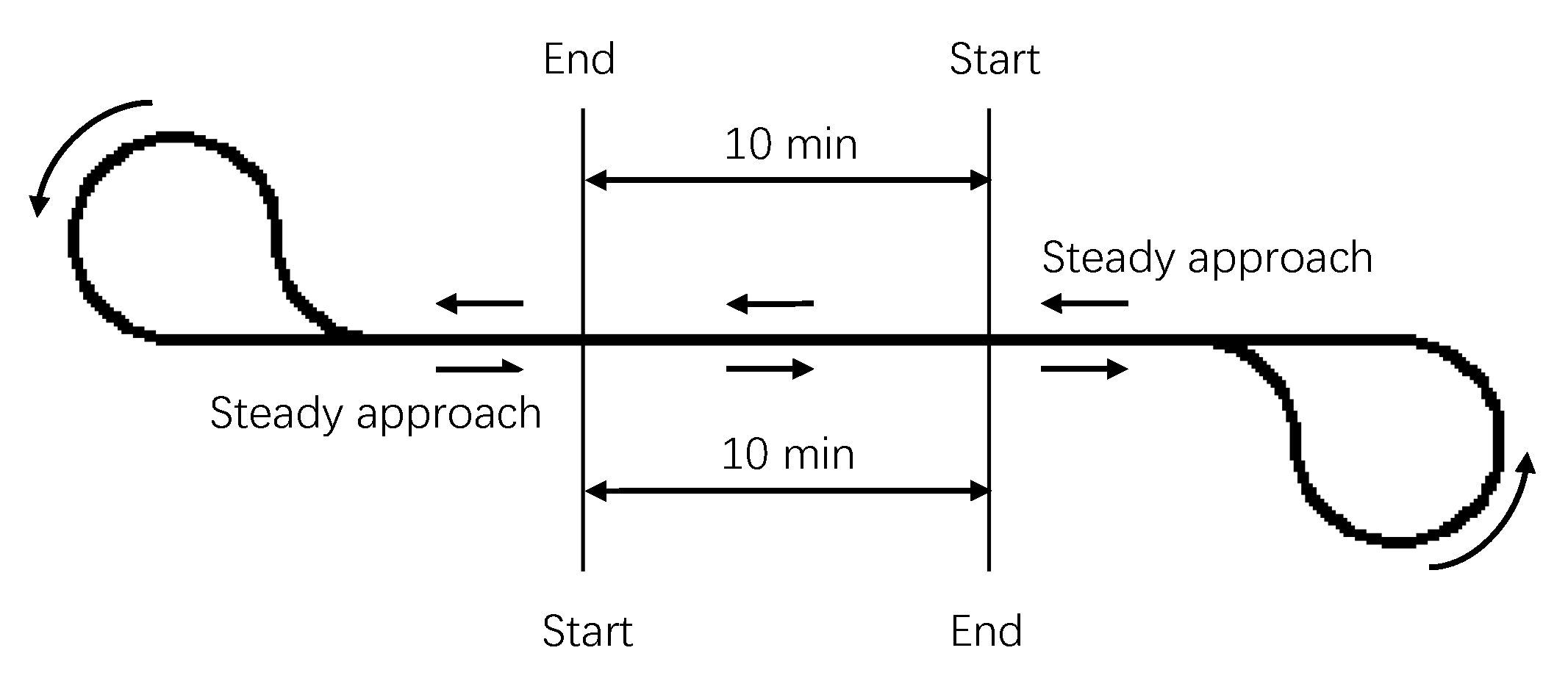
For all double runs, ship heading and ship’s speed over ground were measured by an independent Differential Global Position System (DGPS) installed on the ships. Figure 4 shows an illustration of the ship’s track during the Double Runs. The steady approach was long enough to ensure that the tested ships are in a steady condition prior to the commencement of each speed run. The test duration was 10 min for all speed runs.

3.2. Shaft Torque, Power and Revolution Measurements

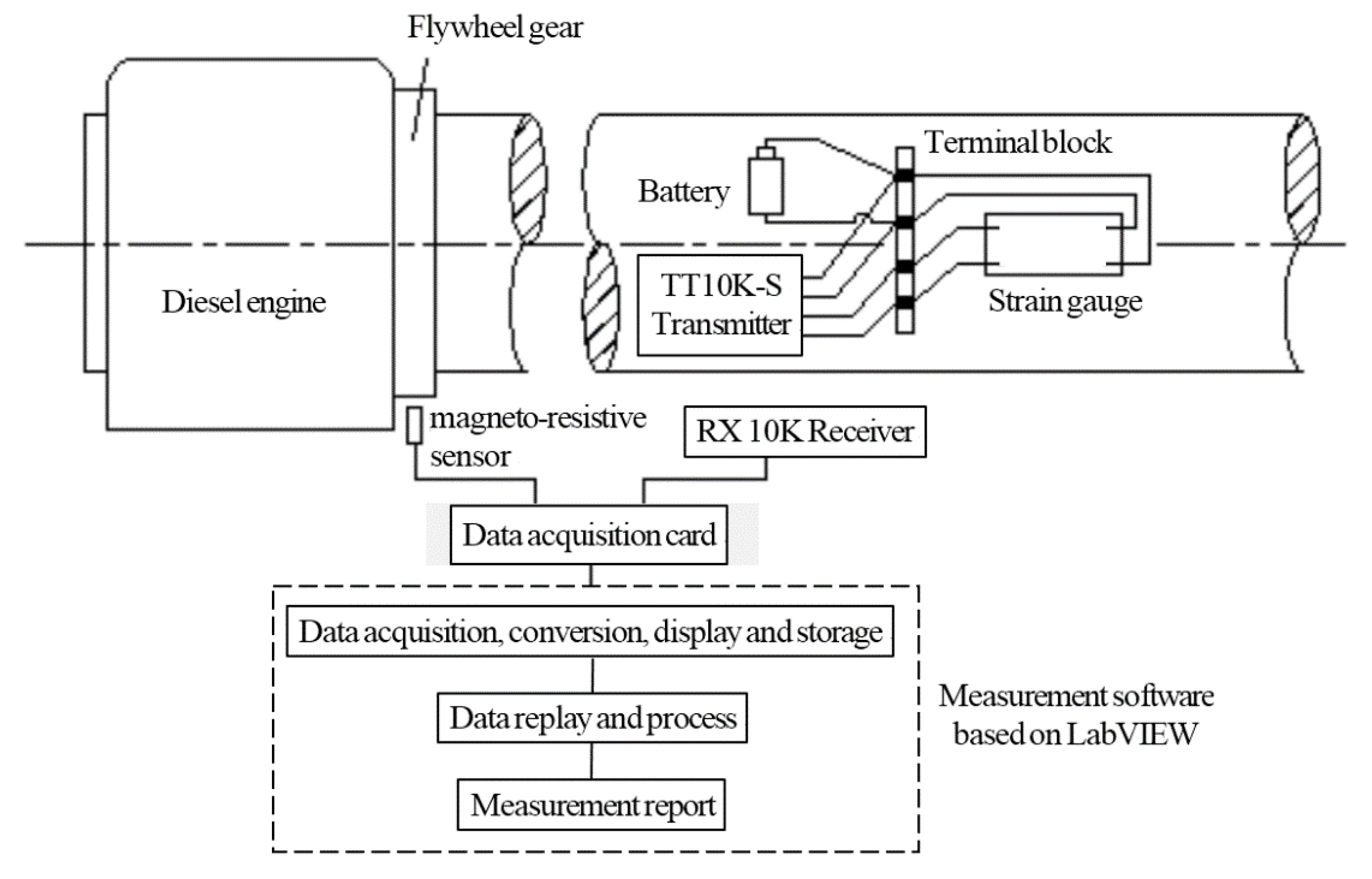
Shaft torque and shaft power were measured by the torque telemetry system installed by CSSRC on the intermediate shaft. The system consists of the strain gauge, terminal block, TT10K torque telemetry system, magneto-resistive sensor, data acquisition card, and measurement software. Figure 5 shows the system composition proposed by Yun et al. [30].

Shaft torque could be obtained by measuring the surface shear strain force. Then, shaft power could be calculated by shaft torque and shaft revolution. As shown in Figure 5, the strain gauge was used to measure the surface shear strain force. One strain gauge is composed of two sets of resistance strain foils along the axis with an angle of 45° and 135°, the four-strain foils are connected by a full-bridge circuit used for converting the change in electric resistance value into a voltage signal. TT10K torque telemetry system (Binsfeld Engineering Inc., Maple City, MI, USA) is composed of 9 V battery, TT10K-S transmitter, and RX 10K receiver. The TT10K-S transmitter is fixed on the shaft and rotates with the shaft. Providing the bridge voltage for the full-bridge circuit of the strain gauge, the measured voltage signal is amplified and transmitted via an antenna. The RX 10K receiver receives and outputs signals in voltage with the range of 0–10 V. The magnitude of the output voltage is proportional to the shaft torque, as shown in the following formula:

$$M_e=\frac{V_{out}}{10}\times M_{FS}=\frac{V_{out}}{10}\times \frac{V_{FS}\pi E\times 4\left(d_o{}^4-d_i{}^4\right)}{16000V_{EXC}{k}_{GF}N\left(1+\mu \right)G_{XMT}{d}_o},$$

(6)

where M_e is shaft torque in $N·m$, M_FS is the full scale torque in $N·m$, $V_{FS}$ is the full scale output (10 V) of system, $E$ is the elasticity modulus of shaft in $N·m{m}^2$, $d_i$ and $d_o$ is the inner and outer diameter of shaft in mm, $V_{EXC}$ is the bridge excitation voltage in V, $k_{GF}$ is the gage factor which is specified on strain gage package, $N$ is the number of active gages which is 4, $\mu$ is the Poisson’s ratio of shaft material, $G_{XMT}$ is telemetry transmitter gain.

Shaft revolution was measured by a magneto-resistive sensor that can perceive the movement of objects within a distance of 3 mm. The magneto-resistive sensor was installed directly to the flywheel and was about 2 mm away from the tooth surface. When the flywheel rotating through a tooth, the magneto-resistive sensor could output an inductive pulse, and the shaft revolution can be calculated based on the number of pulses accumulated in a specified time period as follows:

$$n=\frac{60N}{Mt},$$

(7)

where n is the shaft revolution in r/min, $t$ is the counting time period in seconds; $N$ is the number of pulses accumulated in the counting time period, $M$ is the number of flywheel teeth.

After measuring the output torque and shaft revolution under a certain engine setting, shaft power can be calculated according to the following formula:

$$P_S=\frac{M_e\times n}{9550}.$$

(8)

3.3. Trail Environment Measurement and Data Analysis

Directly simulating the sea trail environment is difficult and time-consuming with current CFD methods and could introduce more unknown uncertainties. Thus, it is better to compare and validate the CFD simulation results with ship performance data in still water. As it is difficult to carry out sea trials under ideal conditions, in practice, certain corrections for environmental conditions, such as water depth, wind, waves, current and deviating ship draught, are performed to achieve the corresponding still water performance of target ships. Therefore, during the speed trials, not only ship speed, shaft power, and shaft revolution, but also the relevant environmental conditions were measured at the same time. Water depth was measured by the ship’s echo-sounder, relative wind speed and direction were measured by the ship’s anemometer and wave data were observed by multiple experienced mariners.

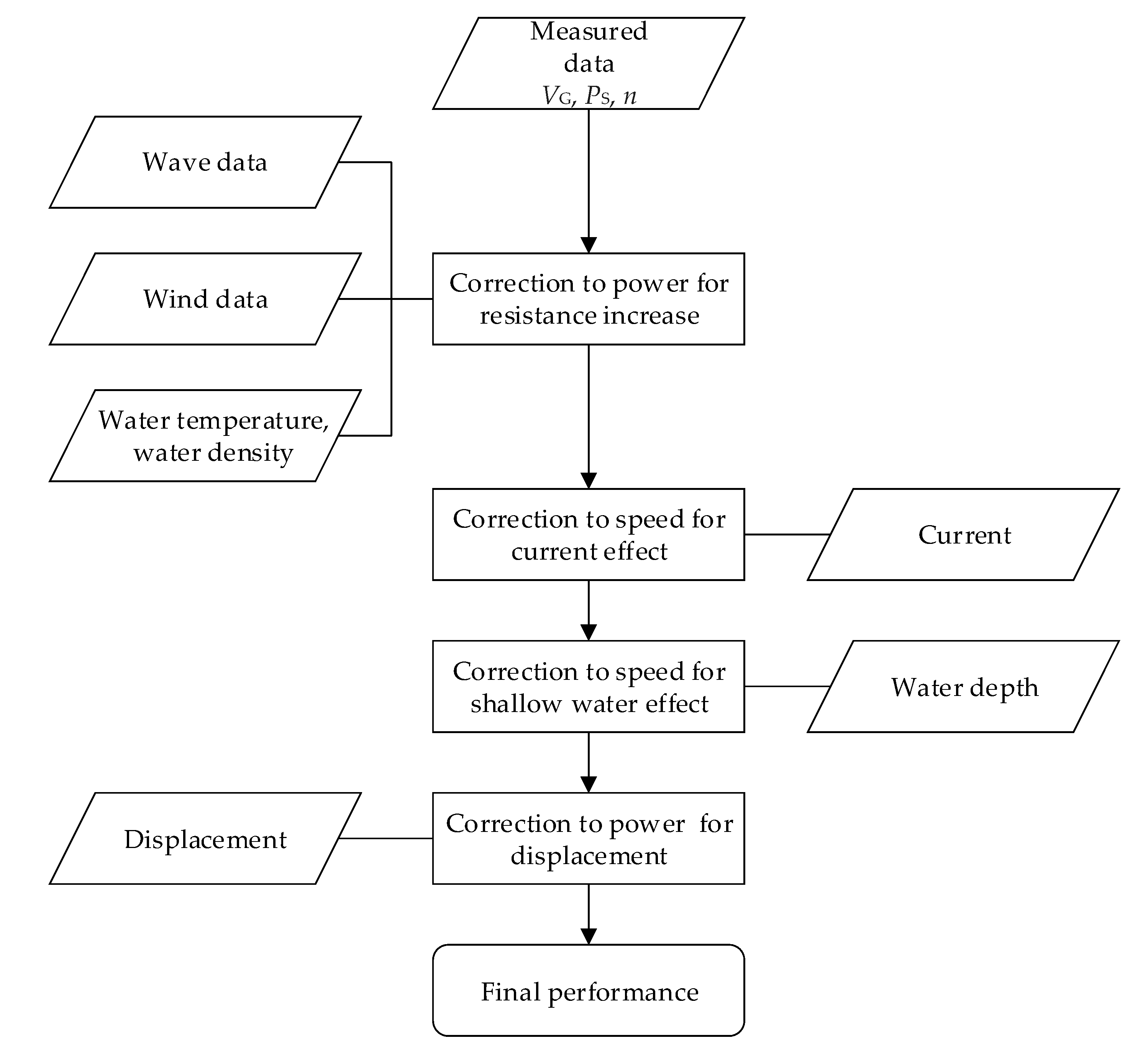
In order to obtain ship’s powering performance under ideal conditions, i.e., no wind, no wave, no current and deep water at 15 °C, the speed trial data were analyzed following the ISO 15016:2015 standard [29]. The analysis procedure includes corrections to power and speed considering the environmental influences. The analysis procedure could be basically divided into several steps, as shown in Figure 6.

For each run, the total resistance increase associated with the measured power is calculated. The total resistance increase comes from relative wind, waves, and deviation of water temperature and water density. Then correction to power due to the total resistance increase is conducted based on the ‘direct power’ method. Additionally, the current effect is corrected by the ‘iterative’ method, the shallow water effect is corrected by the ‘Lackenby’ method and the displacement effect is corrected by Admiral-formula which applied to the power values. Finally, the ship’s performance in terms of ship speed, power and shaft revolution under ideal conditions could be obtained.

4. Results and Analysis

4.1. Scale Effect of Hull-Propeller and Free Surface Interaction

Both model- and full-scale simulations were performed to analyze the scale effect of the ship’s resistance, hull/propeller interaction and free surface’s influence. The scale ratio for the ship model is 25.255 with full scale length of 195 m.

Ahead of the analysis of free surface, scale effect of hull/propeller interaction is presented using double-model simulation results. Four test cases including full scale and model scale simulations with/without propeller were performed without real free surface considered, as listed in

Table 2. Test cases using double-model.

Case	Scale	Propeller	w	Rv	Rp
1	full	without	0.2494	85.37%	14.63%
2	full	with	-	67.66%	32.34%
3	model	without	0.3402	84.73%	15.27%
4	model	with	-	70.43%	29.57%

. A fixed propeller speed was selected at ship speed 14.5 kn, which means that self-propulsion balancing was not carried in this sub-section. That is, the advance coefficient based on ship speed is J_s = 0.861 for both model- and full-scale simulation.

To analyze the scale effect, the proportions of pressure force and viscous force in total resistance are defined as:

$$R_p=\frac{F_p}{F_p+F_v};R_v=\frac{F_v}{F_p+F_v}.$$

(9)

Without propeller, the proportion of viscous force and pressure force shows basically the same for model- and full-scale. The suction effect of the propeller can extremely increase the total force on the hull surface and then changed the ratio of two resistance components. Full-scale simulation leads to higher thrust deduction and has a higher effect on viscous force.

As the boundary layer is relatively thinner (compared to L_pp) for full-scale ship, the decrease of wake fraction (deficit of axial velocity) can also be verified by numerical results. Details of axial and transversal velocity distribution at the propeller plane are shown in Figure 7. At full-scale, the velocity deficit region appears primarily in inner radius and shows a relatively obscure hook-like flow field structure. From the comparison of circumferential averaged axial velocity shown in Figure 8, propeller at full-scale runs in a relatively higher velocity field which has lower thrust and torque coefficients but higher efficiency, as listed in

Table 3. Thrust, torque, and efficiency based on Js.

Scale		Double-Model	VOF
full	KT	0.1414	0.1547
	10 KQ	0.2087	0.2232
	ηB	0.6129	0.5907
model	KT	0.1855	0.1916
	10 KQ	0.2777	0.2830
	ηB	0.5964	0.5900

.

To consider the real free surface effect when a propeller is operating behind the ship, simulations with the VOF model were made for both model- and full-scale ship. Results of propeller performance in Table 3 show that the symmetry boundary condition used in double-model underestimate the propeller force and also the efficiency. For full-scale ship, this discrepancy is relatively larger.

In consideration of the very difference in wake field and its effect on propeller loading, the thrust and torque variations of each propeller blade in its revolution period are plotted for better understanding the scale effect on propulsion. As shown in Figure 9, thrust coefficients for model- and full-scale ship are almost identical with little difference. The maximum single-blade thrust and torque appear at 60° for both model- and full-scale ship (due to the highly skew of propeller), but the minimums appear at 285° for model-scale, which is 15° later than full-scale condition. Also, the discrepancy of thrust and torque between model- and full-scale is small when propeller operating in the region from 285° to 60°, this is due to the smaller magnitude of inflow for propeller blades in portside. The underestimation by double-model can be figured out in Figure 9 especially around the peak of the propeller bearing force.

Additionally, the averaged loading of propeller can be achieved by circumferentially averaging the tangential velocity immediately after the propeller, as follows:

$$G\left(r\right)=\frac{\Gamma \left(r\right)}{\pi VD}=\frac{1}{\pi VDZ}{\displaystyle \oint U_t·rd\theta }.$$

(10)

Higher circulation can be found for most radius at model-scale, which corresponding to higher propeller loads. Discrepancy of curve form only appears at inner radius; circulation shows a sharper drop for model-scale ship close to the hub and a small peak appears at 0.3 R for full-scale condition due to the intensive high-wake region. The red dashed lines in Figure 10 refer to the circulation distribution obtained by the VOF model, both model- and full-scale results show slightly higher circulation along the whole radius of propeller compared to the results from the double-model. But the circulation distributions remain almost the same for two free surface treatments except that real free surface effect can smoothing the load distribution for model-scale propeller at 0.85 R.

The difference of propeller loading distribution can also be figured out by comparing the time-averaged axial velocity immediately behind the propeller. From the left column (model-scale) and right column (full-scale) of Figure 11, we can find out that in full-scale condition, the propeller has a larger high loading region and can produce a more uniform wake. The low-velocity zone near the hub is also smaller for full-scale ship, which is in coincidence with the ship wake. By comparing the results from two free surface treatments, the free surface boundary effect only appears in the upper half of the propeller wake and will not change the flow structure.

The time-averaged axial velocity on the central longitudinal section (Y = 0) is shown in Figure 12. Propeller at full-scale can produce a large range of high velocity region compared to the model-scale results. But the low velocity region after the boss cap is larger for full-scale case. The difference of two free surface treatments appears when the VOF model can produce lower axial velocity near the free surface in Y = 0 plane.

The instantaneous flow field is characterized in Figure 13 using nondimensional Q-criterion defined as:

$$\overline{Q}=\frac{Q}{{(U/L)}^2}.$$

(11)

After nondimensionalization, vortex structures at the model- and full-scale become comparable with a same value of $\overline{Q}$. For both model- and full-scale ship, vortex sheet in upper half of propeller wake undergoes flow fields with higher velocity gradients and are more difficult to main stable vortex structure. This phenomenon is also affected by the free surface. When the tip vortex reaches the low velocity region close to the free surface, it is more likely to break up to small vortex structures. This progress will certainly facilitate the turbulence dissipation and then speed up the mixing of the velocity field in the propeller wake. The breakup of tip vortex for full-scale ship comes relatively later and can maintain a more stable structure when translating to the intermediate wake. One explanation is that, for full-scale ship, the velocity deficit region locates limitedly in the inner radius region. So that the tip vortex undergoes a more uniform velocity field when translating to downstream. Another reason is the interaction between the propeller vortex sheet and ship shedding vortex. For full-scale ship, the shedding vortex from the flow separation of the hull boundary layer locates in the inner and upper region of the propeller disk which is relatively far from the propeller’s main loading area and has little interaction with propeller tip vortex.

A comparison between Figure 13a,c reflects the difference of free surface boundary conditions on propeller vortex evolution. The tip vortex resulting from the double-model is more likely to break up, and this may be caused by the reflection effect of the symmetry boundary. But the VOF model can produce more real interaction between free surface and vortex transportation, thus results in more stable structures. For full-scale cases, a similar difference can also be figured out.

The wave profiles along the Y = 0 plane at model- and full-scale conditions are plotted in Figure 14. The wave profiles are almost the same for two conditions with a slight discrepancy at crests and troughs. The nondimensional wave height is greater for the model-scale ship. The propeller’s effect on wave profile is negligible compared to the wave-making effect of ship stern.

4.2. Self-Propulsion Performance Prediction Compared to Sea Trail Results

In the previous sub-section, the scale effect of the ship’s resistance and hull/propeller interaction considering different free surface treatments were analyzed at a fixed propeller rotation speed without a rudder. In this sub-section, we provide the results of full-scale self-propulsion performance prediction at the same condition with sea trail tests with a rudder installed. Due to the large amount of computational cost of the VOF method, it preferred to use double-model method when the free surface effect is negligible. So, both double-model and VOF methods were adopted in this sub-section to quantify the effect of free surface treatment on powering performance prediction.

4.2.1. Self-Propulsion Balance Condition

In order to achieve the self-propulsion balance, a series of propeller speeds were evaluated. For full-scale case, there is no friction force correction, so the self-propulsion balance can be achieved by equalizing propeller thrust $T$ and ship resistance with propeller $R_{SP}$.

$$T=R_{SP}.$$

(12)

With the VOF method, $T$ and $R_{SP}$ could be obtained directly from the integration of force on propeller and hull surface respectively. However, an additional balance correction is needed for double-model method. From the results from the previous sub-section, it could be concluded that the free surface treatments have influence on self-propulsion balance from three aspects:

• Ship resistance
• Propeller performance
• Ship added resistance induced by propeller

The influence on bare hull resistance, nominal wake and propeller loading at a fixed propeller speed has been introduced in the previous section, while the effect on propeller performance at different revolutions is shown in Figure 15a. In accordance with the result of the previous sub-section, the propeller thrust and torque resulted from the VOF method is always larger than that from double-model treatment. This kind of difference may come from two sources: one is the difference in propeller inflow; another is the free surface boundary condition itself.

The influence of propeller induced resistance, as defined in Equation (13), is shown in Figure 15b, where $R_t$ refers to ship resistance in calm water without propeller. The resultant value of $\Delta R$ is relatively higher with the VOF method. Traditionally, the effect of free surface treatment on $\Delta R$ is assumed negligible when performing the self-propulsion balance [21] for cases in the design draft. However, as sea trails test is always performed in a light ballast draft, where propeller rotates close to the free surface, this discrepancy should not be ignored.

$$\Delta R=R_{SP}-R_t.$$

(13)

Considering all the possible influence from free surface treatments, a modified self-propulsion balance correction method in ship scale is proposed, as shown in Equation (14).

$$\begin{array}{cc}\hfill T^{VOF}=& R_{SP}^{VOF}=R_T^{VOF}+\Delta R^{VOF}\hfill \\ \hfill T^{DM}+{\Delta }_T^{VOF}=& \left(R_T^{DM}+{\Delta }_{R_T}^{VOF}\right)+\left(\Delta R^{DM}+{\Delta }_{\Delta R}^{VOF}\right)\hfill \\ \hfill T^{DM}+{\Delta }_T^{VOF}=& R_{SP}^{DM}+{\Delta }_{R_T}^{VOF}+{\Delta }_{\Delta R}^{VOF}\hfill \end{array},$$

(14)

where the superscript DM refers to double-model treatment and VOF means the VOF treatment. ${\Delta }_{\phi }^{VOF}$ refers to the discrepancy between VOF and double model treatment on quantity $\phi$, that is ${\Delta }_{\phi }^{VOF}={\phi }^{VOF}-{\phi }^{DM}$.

Equation (14) represents the effect of free surface treatment on full-scale self-propulsion balance by three components: Thrust ${\Delta }_T^{VOF}$, bare hull resistance ${\Delta }_{R_T}^{VOF}$, and propeller induced hull resistance ${\Delta }_{\Delta R}^{VOF}$. Then, free surface correction factors ${\epsilon }_T,{\epsilon }_R,{\epsilon }_{R_T},{\epsilon }_{\Delta R}$ are introduced in Equation (15), which represent the correction to the calculated thrust and resistant of ship respectively.

$${\epsilon }_T=\frac{T^{VOF}-T^{DM}}{T^{DM}},{\epsilon }_{R_{SP}}=\frac{R_{SP}^{VOF}-R_{SP}^{DM}}{R_{SP}^{DM}},{\epsilon }_{R_T}=\frac{R_T^{VOF}-R_T^{DM}}{R_T^{DM}},{\epsilon }_{\Delta R}=\frac{\Delta R^{VOF}-\Delta R^{DM}}{\Delta R^{DM}}.$$

(15)

The influence of free surface treatments on propeller trust, torque and propeller induced resistance are relatively small compared to the effect on bare hull resistance, but still has non-negligible effect in this test case. The effect of free surface treatment increases with propeller speed and the correction factors are not constants for different advance ratio. For the cases where there is no detailed comparison between different free surface treatments, some easy to use regression models could be adopted to predict the correction factors. With known correction factors, the self-propulsion balance condition for double-model method could be simplified to Equation (16).

$$\begin{array}{ll}{T}^{DM}\left(1+{\epsilon }_T\right)& =R_{SP}^{DM}\left(1+{\epsilon }_{R_{SP}}\right)=R_T^{DM}\left(1+{\epsilon }_{R_T}\right)+\Delta R^{DM}\left(1+{\epsilon }_{\Delta R}\right)\\ & =R_T^{DM}\left({\epsilon }_{R_T}-{\epsilon }_{\Delta R}\right)+R_{SP}^{DM}\left(1+{\epsilon }_{\Delta R}\right)\end{array}.$$

(16)

4.2.2. Powering Performance Prediction

Results of the powering performance prediction from full-scale CFD simulations, towing tank tests, and sea trails are presented in this sub-section. As stated above, when self-prolusion balance was achieved by interpolating propeller speed to satisfy Equation (13) or Equation (16), the delivery power at a given ship speed could be calculated by

$$P_D=2\pi nQ,$$

(17)

where $n$ is the propeller speed and $Q$ is the torque.

Usually, the hull roughness was ignored in model-scale ship resistance and self-propulsion prediction. However, in this sub-section, the full-scale simulation will be compared to the statistical sea trail results according to the analysis procedure proposed in Section 4. Thus, the roughness effect plays an important role to the increase of friction resistance and ship’s shaft power. There have two approaches to take roughness effect into consideration according to the most recent work of Niklas and Pruszko [31]. One is the most widely used Bowden–Davison formula [6] as shown in Equation (18), where $k_s$ is the roughness height and $L_{WL}$ is the length of waterline. Therefore, the increase of friction resistance could be obtained by multiplying $\Delta C_F$ by $\frac{1}{2}\rho V_s^{2}S$.

$$\Delta C_F=105\left(\frac{k_s}{L_{WL}}\right)-0.64.$$

(18)

Another one is to introduce the roughness effect directly into the wall function of the turbulence model. In this way, it is assumed that roughness could increase the local turbulence near the wall, thus could change the velocity profile in the log-law region. Recently, this method was widely used in many full-scale simulation practices, like Demirel et al. [32], Niklas and Pruszko [31]. According to their reported results, the selection of the turbulence model, grid arrangement and roughness model have a significant effect on the prediction results. According to the conclusion of Niklas and Pruszko [31], it is difficult to assess to what extent the discrepancies result from the roughness model and what is the influence of different turbulence models applied. As the roughness effect is not the focus of this article, we prefer the Bowden–Davison formula to avoid introducing more complicated uncertainty sources to CFD simulation. According to our historical data, the increase friction resistance coefficient was equal $\Delta C_F=0.1779·{10}^{-3}$ with roughness height assumed equal to $k_s=90 \mathsf{\mu }\mathrm{m}$.

It is well known that the treatment of hull resistance, propeller performance, and hull-propeller interaction will significantly affect the result of self-propulsion balance and thus the resulted powering performance of a ship. So, a detailed comparison of the consideration of roughness and free surface correction was performed to quantify the influence.

Table 4. Tested cases.

Case NO.	Free Surface Treatment	Roughness	${\mathsf{\Delta }}_{{\mathit{R}}_{\mathit{T}}}^{\mathit{V}\mathit{O}\mathit{F}}$	${\mathsf{\Delta }}_{\mathit{T}}^{\mathit{V}\mathit{O}\mathit{F}}$	${\mathsf{\Delta }}_{\mathsf{\Delta }\mathit{R}}^{\mathit{V}\mathit{O}\mathit{F}}$
1	VOF	No	-	-	-
2	VOF	Yes	-	-	-
3	Double-Model	No	Yes	No	No
4	Double-Model	Yes	Yes	No	No
5	Double-Model	Yes	Yes	Yes	No
6	Double-Model	Yes	Yes	No	Yes
7	Double-Model	Yes	Yes	Yes	Yes

shows all the tested cases included with different roughness and free surface corrections. When the free surface was treated by the VOF method, there have no other free surface corrections. When the free surface was treated by a double-model method, free surface corrections are considered in self-propulsion balance according to Equation (16). The correction on bare hull resistance is mandatory while corrections on trust and propeller induced resistance are optional.

Self-propulsion points along with ship resistance, propeller trust and torque obtained by different approaches are presented in Figure 16. Figure 17 presents a comparison of the balanced propeller speed, torque, thrust and delivery power by the relative percentages of the test case 2 (VOF method with roughness). It could be figured out that the roughness effect has a significant effect on ship resistance and will change the self-propulsion point by 1.6% for RPS. Thus, it has a larger effect on propeller torque (5.8%) and the resultant delivery power (7%) prediction. For the double-model method, only correcting the bare hull resistance leads to a slight underestimation of balanced propeller speed (about 0.6%) and the delivery power (3%). From the comparison of cases 6 and 7, the leave-out-of-thrust-correction (case 6) overestimates the balanced RPS. Because the increase of propeller speed compensates the correction to propeller torque, the resultant delivery power only shows 1.6% higher than case 7.

The results of powering performance prediction obtained by several approaches mentioned above were compared to the extrapolated self-propulsion result from model test and statistical sea trail results. In this article, sea trail results were achieved by collecting nine times of sea trial test for nine new-build ships with the same hull form, propeller and appendages. The analysis of all the sea trails data followed the same procedure as stated in Section 3 to avoid any additional uncertainties. Figure 18 shows the uncertainty of sea trail results at different ship speeds, the uncertainty here is defined by the standard deviation of power-speed prediction result of the 9 tested ships. The overall statistical uncertainty along all speeds does not exceed 2% of the mean value and the estimated uncertainty due to weather effect could also be controlled under 2% according to the ITTC guidelines.

Figure 19 presents the model test results, sea trail results with confidence interval and the seven predictions. The extrapolated towing tank result overestimates the delivery power by approximately 2.4% compared to the statistical sea trail results. At service speed, all five CFD predictions with roughness effect included show good agreement (between −1.1% and 2.4%) with sea trail results especially for Case 2 and Case 7, where both roughness effect and free surface effect were fully considered. Approximately 6–7% discrepancy was found for cases that did not take roughness effect into consideration. The very little difference between the VOF method and the corrected double—model method mainly comes from the interpolating error and regression procedure of correction factors. Also, the correction method was applied to low speed prediction to validate its extensibility. As a result, the numerical method with double-model and free surface correction slightly overestimates the delivery power by about 2.5–4.8% compared to sea trails result in the consideration of hull roughness. That is, at low speed, the overestimation of numerical prediction is higher than that at design speed. Unfortunately, the genuine source of the modeling or numerical uncertainties is difficult to access with the present study, more systematic and sophisticated efforts should be made to quantify the uncertainties in the future. It is one of the most important issues regarding both ship CFD methods and full scale performance predictions.

5. Discussion

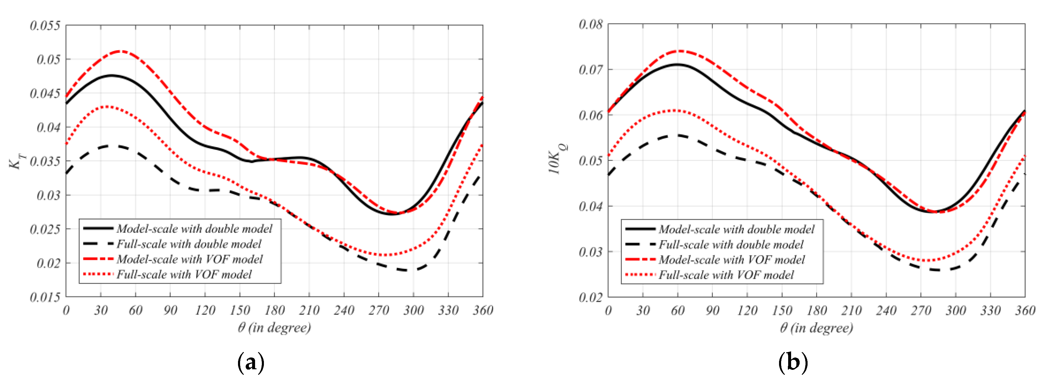
Numerical simulations are performed for a commercial bulk carrier in light ballast condition to investigate the complicated interaction around the propeller and to predict the self-propulsion performance. Free surface effects are considered with double-model and VOF model respectively to quantify the difference between the two methods. Scale-effect of hull-propeller interaction under the free surface is detailed presented by wake field, propeller unsteady force and trailing vortex transportation.

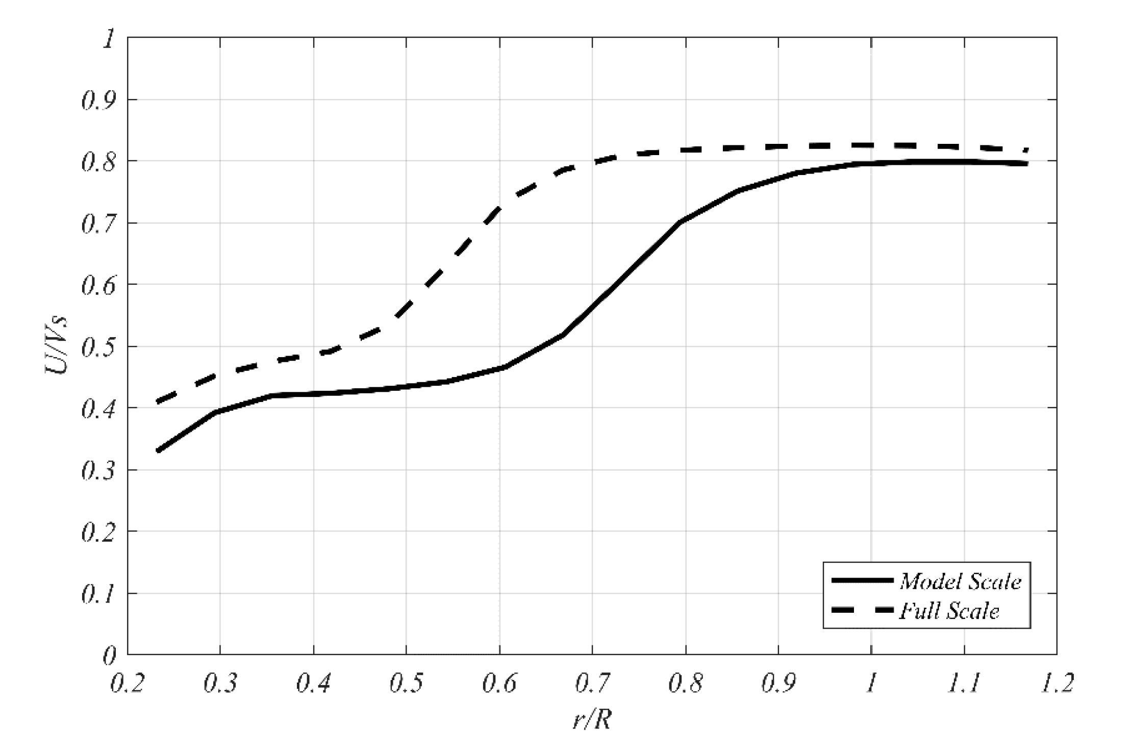
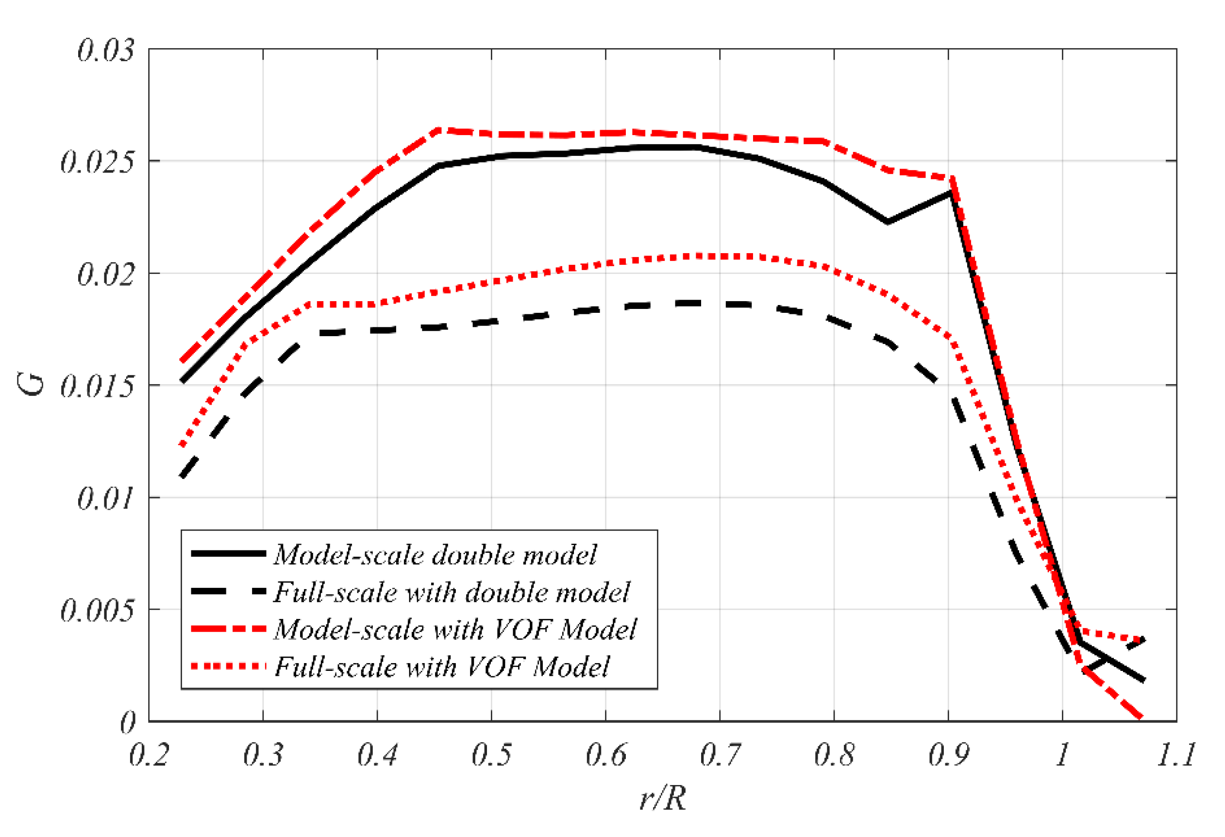
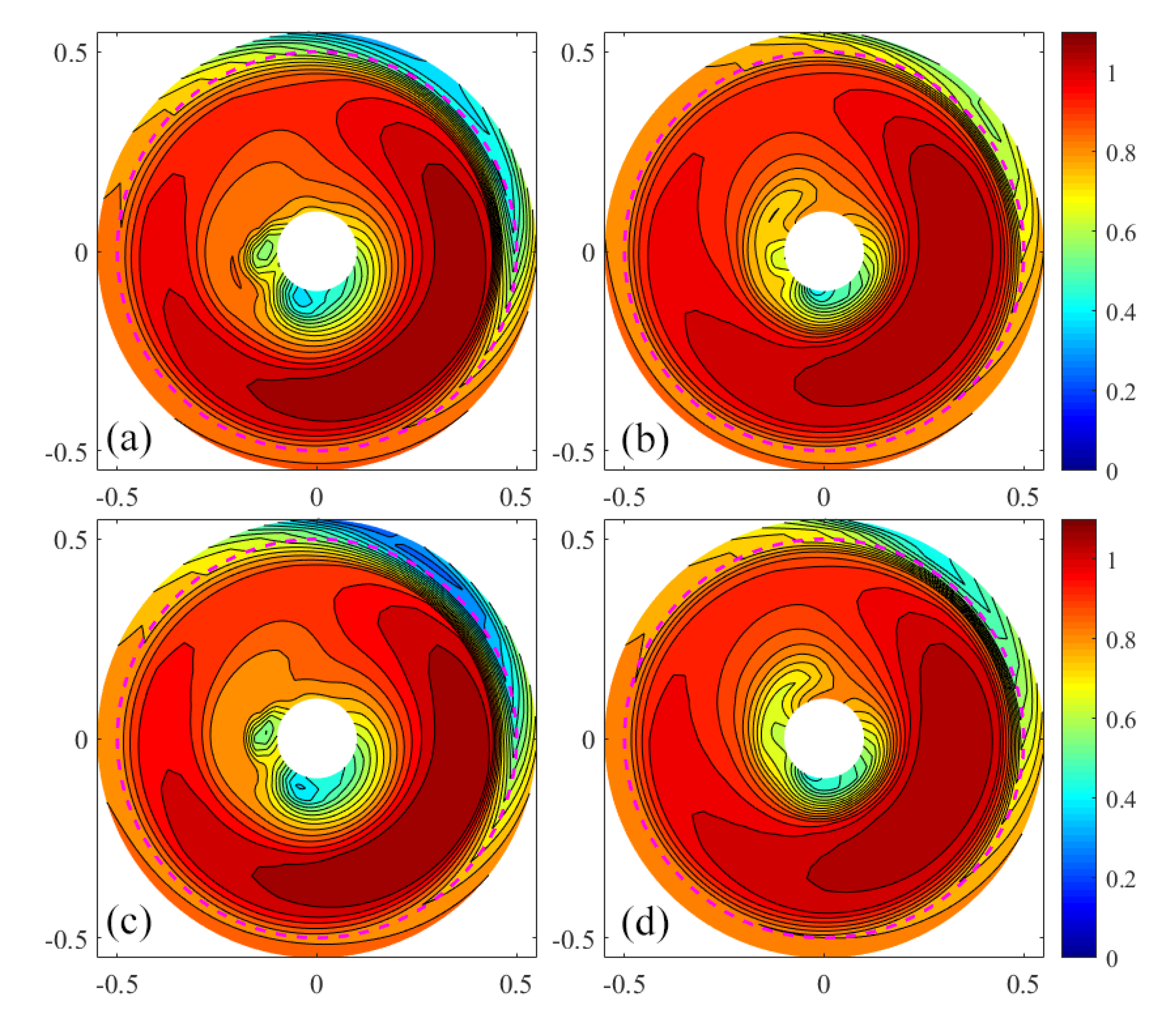
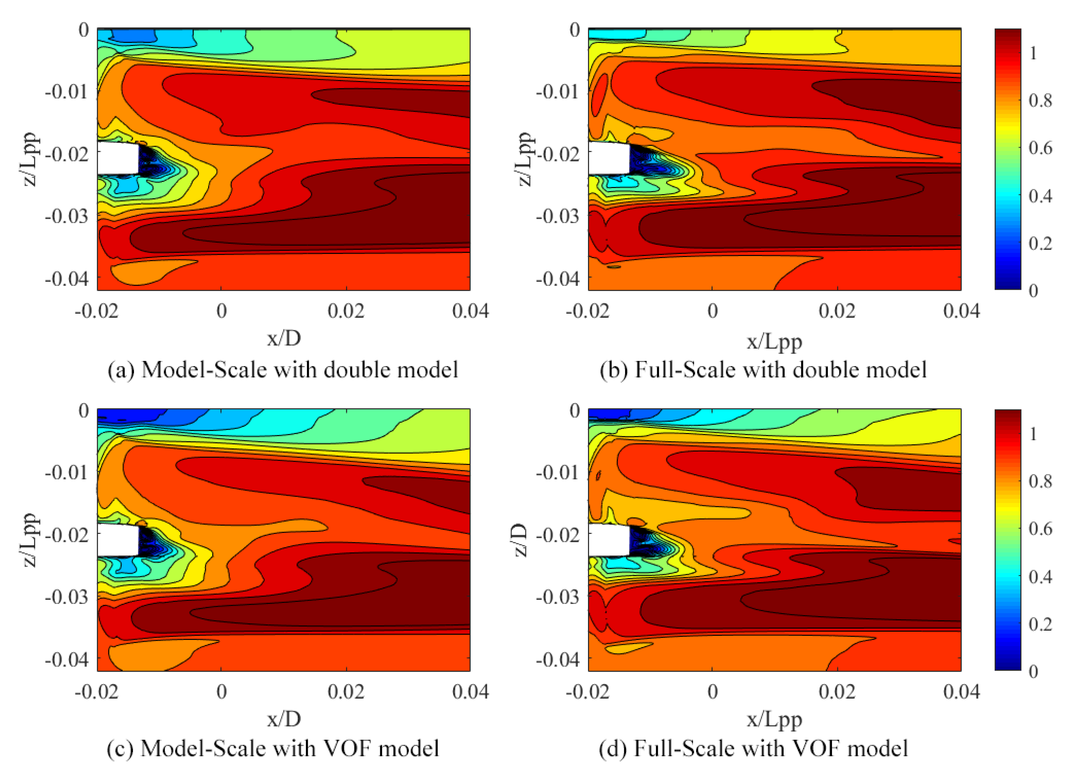
The most significant scale effect appears in the ship wake. Full-scale simulation can produce a smaller high wake region around the shaft, which is the main source of the difference in propeller hydrodynamic performance. The overall circumferential axial velocity is higher for full-scale ship and makes propeller working with a high advance ratio. The propeller loading is significantly higher for model-scale ships according to the analysis of circulation distribution and downstream flow fields. Free surface treatments have non-negligible effect on propeller loading. Compared to the most realistic modeling of the free surface by the VOF model, the double-model treatment apparently underestimates the propeller loading. This phenomenon should be considered in the prediction of self-propulsion performance especially for ballast condition.

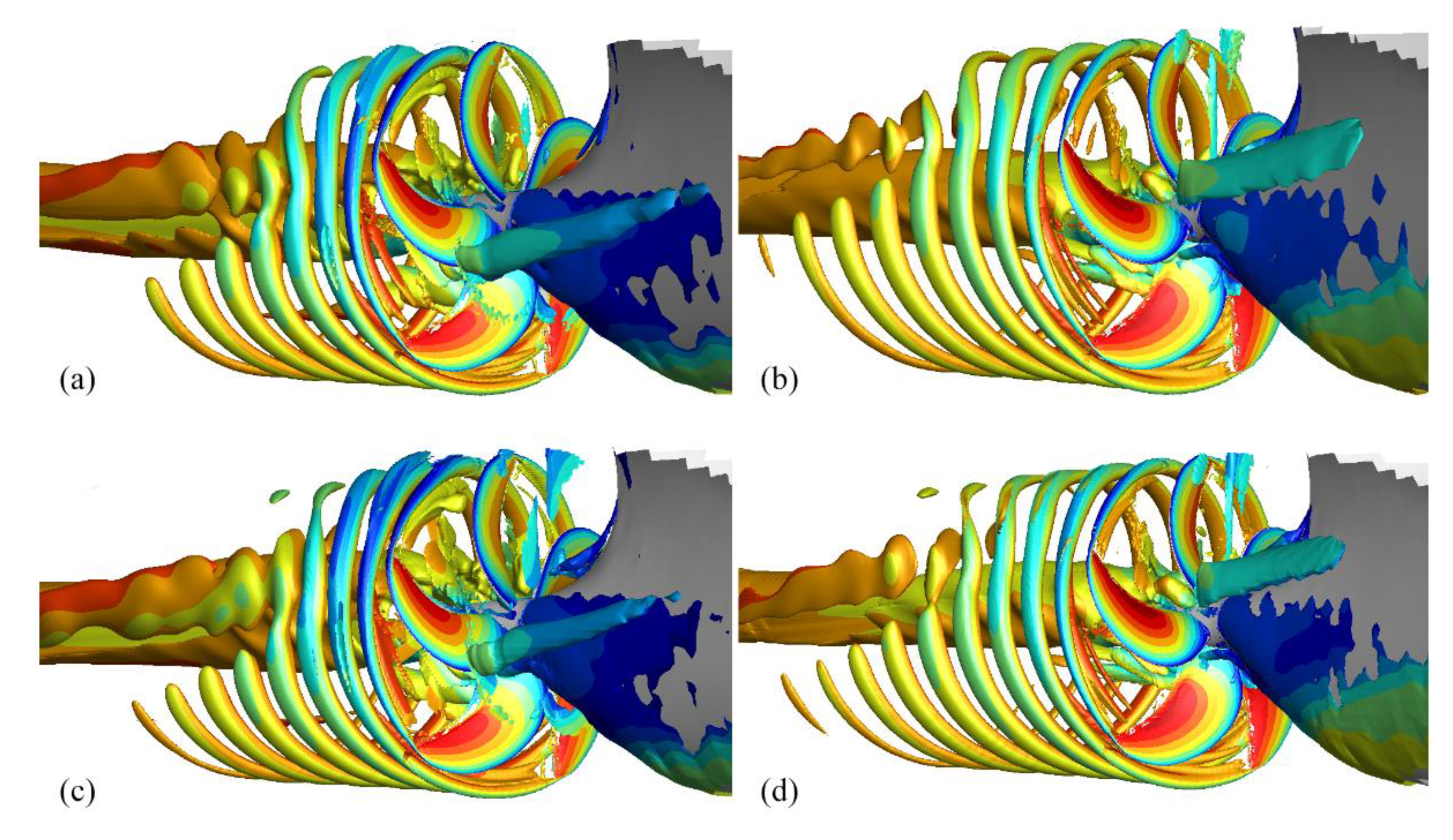
A non-dimensional vortex recognition criterion is introduced to make the vortex structure comparable at different Reynolds numbers. Full-scale and model-scale ship can produce similar trailing vortex sheet, which is more stable at full-scale condition due to the more favorable inflow. The interaction of ship shedding vortex, tip vortex and free surface impact the evolution of the vortex sheet. So, scale effect also originates from ship’s boundary layer separation. Free surface treatments have a small effect on the propeller vortex sheet, the symmetry free surface boundary condition could make propeller tip vortex more vulnerable to break up in downstream.

It is well known that considering free surface with VOF in self-propulsion simulation requires a large amount of computational resources. Therefore, we compared the effect of free surface treatments on ship’s self-propulsion balance to offer some suggestions for engineering practice with a more time-saving double-model approach. It could be concluded that the simplification of free surface treatment does not only affect the wave-making resistance for bare hull but also the propeller performance and propeller induced ship resistance. In this case, ignore the free surface correction on propeller performance and propeller induced resistance brings up to 5% more uncertainty to the result of power prediction. According to the simple treatment in this article, roughness is another important factor in full-scale simulation because it has up to approximately 7% effect on the delivery power. As have been discussed by other researchers, the appropriate direct modeling of roughness in CFD method still remains questionable and more experiments, numerical studies and modeling method developments should be made in the future.

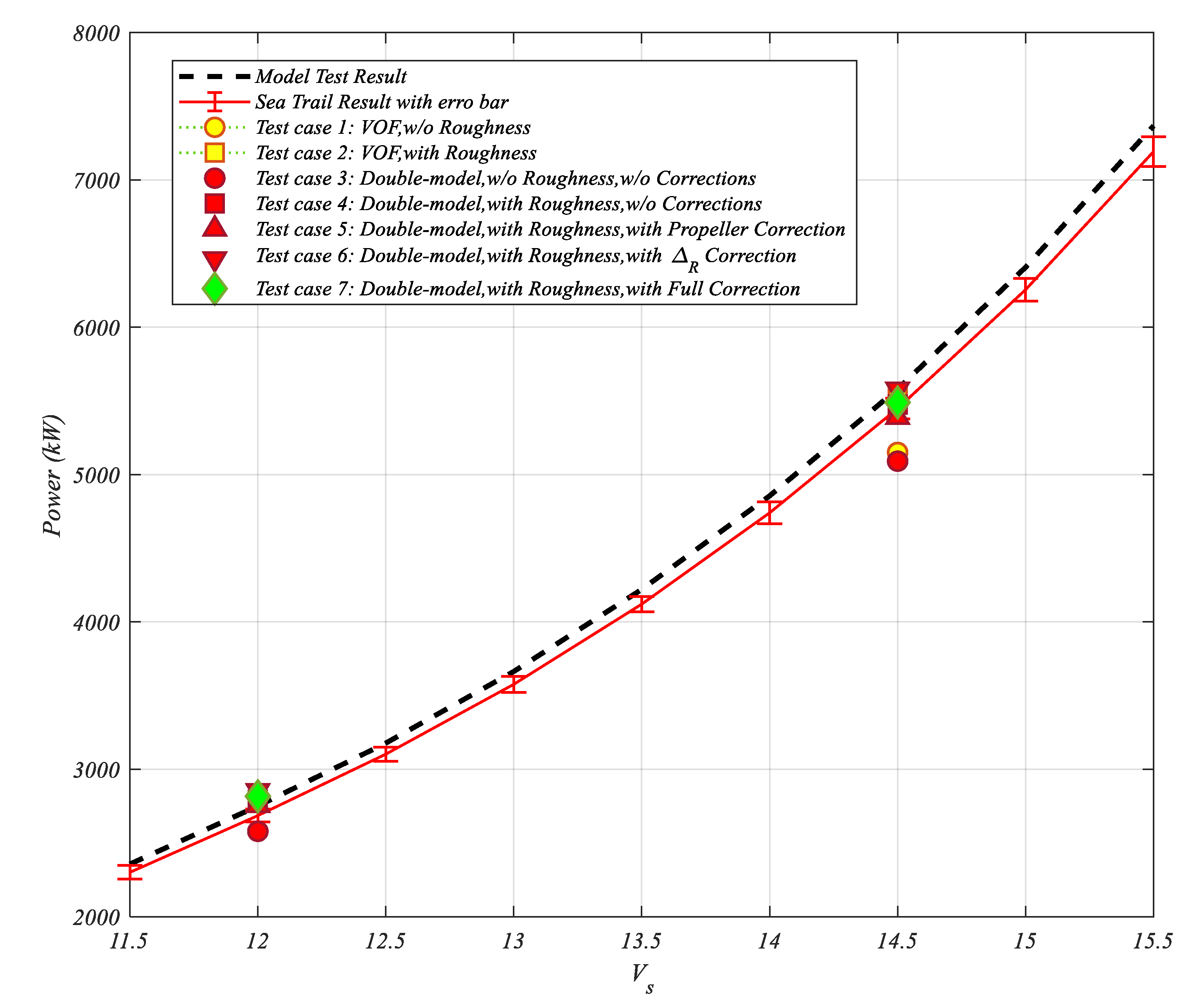
The validation data provided by 9 times of sea trail test shows good quality with low uncertainty. For this ship, the towing tank prediction overestimates the power at service speed. Because the detailed information of the extrapolating method is unknown to us in this research, we prefer the statistical sea trial results to validate the CFD predictions. As a result, the numerical simulations of full-scale ship self-propulsion show good agreement with the sea trail data especially for cases that have considered both roughness and free surface effects. Predictions without the consideration of hull surface roughness significantly underestimates the delivery power.

In the future, more scientific studies should be performed to deeply investigate the mechanism of these mutual interactions. Quantitative, statistical or analytical models should be established in the future for better application to industrial design activities. Numerous efforts shall be made in the future to investigate more influence factors like wall roughness modeling, weather condition, and ship motions effect. Also, more detailed and systematical analysis of uncertainty in full-scale simulation and sea trails should be performed in the future to identify the confidence level of currently used predicting methodology.

References

1. Larsson, L.; Stern, F.; Visonneau, M. Numerical Ship Hydrodynamics—An Assessment of the Gothenburg 2010 Workshop; Springer: Dordrecht, The Netherlands, 2014. [Google Scholar]
2. Pereira, F.; Vaz, G.; Eca, L. Verification and Validation Exercises for the Flow Around the KVLCC2 Tanker at Model and Full-Scale Reynolds Numbers. Ocean Eng. 2017, 129, 133–148. [Google Scholar] [CrossRef]
3. Duvigneau, R.; Visonneau, M.; Gan, B.D. On the role played by turbulence closures in hull shape optimization at model and full scale. J. Mar. Sci. Technol. 2003, 8, 11–25. [Google Scholar] [CrossRef]
4. Leer-Andersen, M.; Larsson, L. An experimental/numerical approach for evaluating skin friction on full-scale ships with surface roughness. J. Mar. Sci. Technol. 2003, 8, 26–36. [Google Scholar] [CrossRef]
5. Bhushan, S.; Xing, T.; Carrica, P.; Stern, F. Model- and Full-Scale URANS Simulations of Athena Resistance, Powering, Seakeeping, and 5415 Maneuvering. J. Ship Res. 2009, 53, 179–198. [Google Scholar]
6. ITTC. 1978 ITTC Performance Prediction Method; ITTC: Zürich, Switzerland, 2014. [Google Scholar]
7. Min, K.-S.; Kang, S.-H. Study on the form factor and full-scale ship resistance prediction method. J. Mar. Sci. Technol. 2010, 15, 108–118. [Google Scholar] [CrossRef]
8. Katsui, T.; Asai, H.; Himeno, Y.; Tahara, Y. The proposal of a new friction line. In Proceedings of the Fifth Osaka Clolloquium on Advanced CFD Applications to Ship Flow and Hull from Design, Osaka, Japan, 14–15 March 2005. [Google Scholar]
9. Eca, L.; Hoekstra, M. The numerical friction line. J. Mar. Sci. Technol. 2005, 13, 328–345. [Google Scholar] [CrossRef]
10. Park, D.-W. A study on the effect of flat plate friction resistance on speed performance prediction of full scale. Int. J. Nav. Archit. Ocean Eng. 2015, 7, 195–211. [Google Scholar] [CrossRef] [Green Version]
11. Castro, A.M.; Carrica, P.M.; Stern, F. Full scale self-propulsion computations using discretized propeller for the KRISO container ship KCS. Comput. Fluids 2011, 51, 35–47. [Google Scholar] [CrossRef]
12. Satrke, B.; Bosschers, J. Analysis of scale effects in ship powering performance using a hybrid RANS-BEM approach. In Proceedings of the 29th Symposium on Naval Hydrodynamics, Gothenburg, Sweden, 26–31 August 2012. [Google Scholar]
13. Lin, T.-Y.; Kouh, J.-S. On the scale effect of thrust deduction in a judicious self-propulsion procedure for a moderate-speed containership. J. Mar. Sci. Technol. 2015, 20, 373–391. [Google Scholar] [CrossRef]
14. Wang, Z.Z.; Xiong, Y.; Wang, R.; Shen, X.-R.; Zhong, C.-H. Numerical study on scale effect of nominal wake of single screw ship. Ocean Eng. 2015, 104, 437–451. [Google Scholar] [CrossRef]
15. Guo, C.; Zhang, Q.; Shen, Y. A non-geometrically similar model for predicting the wake field of full-scale ships. J. Mar. Sci. Appl. 2015, 14, 225–233. [Google Scholar] [CrossRef]
16. Park, S.; Oh, G.; Hyung Rhee, S.; Koo, B.-Y.; Lee, H. Full scale wake prediction of an energy saving device by using computational fluid dynamics. Ocean Eng. 2015, 101, 254–263. [Google Scholar] [CrossRef]
17. Shen, H.-L.; Enock Omweri, O.; Su, Y.-M. Scale effects for rudder bulb and rudder thrust fin on propulsive efficiency based on computational fluid dynamics. Ocean Eng. 2016, 117, 199–209. [Google Scholar]
18. Carrica, P.M.; Mofidi, A.; Martin, E. Progress toward direct CFD simulation of Maneuvers in waves. In Proceedings of the VI International Conference on Computational Methods in Marine Engineering (Marine 2015), Rome, Italy, 15–17 June 2015; pp. 327–338. [Google Scholar]
19. Shen, Z.; Wan, D.; Carrica, P.M. Dynamic overset grids in OpenFOAM with application to KCS self-propulsion and maneuvering. Ocean Eng. 2015, 108, 287–306. [Google Scholar] [CrossRef]
20. Jasak, H.; Vukcevic, V.; Gatin, I.; Lalovic, I. CFD validation and grid sensitivity studies of full scale ship self propulsion. Int. J. Nav. Archit. Ocean Eng. 2019, 11, 33–43. [Google Scholar] [CrossRef]
21. Gaggero, S.; Villa, D.; Viviani, M. An extensive analysis of numerical ship self-propulsion prediction viaa coupled BEM/RANS approach. Appl. Ocean Res. 2017, 66, 55–78. [Google Scholar] [CrossRef]
22. Sánchez-Caja, A.; Martio, J.; Saisto, I.; Siikonen, T. On the enhancement of coupling potential flow models to RANS solvers for the prediction of propeller effective wakes. J. Mar. Sci. Technol. 2015, 20, 104–117. [Google Scholar] [CrossRef]
23. Sun, W.; Yang, L.; Wei, J.; Chen, J.; Huang, G. Numerical analysis of propeller loading with a coupling RANS and potential approach. Proc. Inst. Mech. Eng. Part C J. Mech. Eng. Sci. 2019, 233, 6383–6396. [Google Scholar] [CrossRef]
24. Mikkelsen, H.; Steffensen, M.L.; Ciortan, C.; Walther, J.H. Ship Scale Validation of CFD Model of Self-Propelled Ship. In Proceedings of the VIII International Conference on Computational Methods in Marine Engineering (Marine 2019), Gothenburg, Sweden, 13–15 May 2019. [Google Scholar]
25. Wang, C.; Sun, S.; Li, L.; Ye, L. Numerical prediction analysis of propeller bearing force for full-scale hull–propeller–rudder system. Int. J. Nav. Archit. Ocean Eng. 2016, 8, 589–610. [Google Scholar] [CrossRef] [Green Version]
26. Visonneau, M. A step towards the numerical simulation of viscous flows around ships at hfull scale—Recent achievements within the European Union Project EFFORT. In Proceedings of the 4th International Conference on Marine Hydrodynamics (Marine CFD 2005), London, UK, 30–31 March 2005. [Google Scholar]
27. Ponkratov, D. Proceedings of the 2016 Workshop on Ship Scale Hydrodynamic Computer Simulations; Lloyd’s Register: Southampton, UK, 25 November 2016; Available online: https://www.lr.org/en/events/ (accessed on 2 January 2020).
28. Ponkratov, D.; Zegos, C. Validation of Ship Scale CFD Self-Propulsion Simulation by the Direct Comparison with Sea Trials Results. In Proceedings of the Fourth International Symposium on Marine Propulsors, Asutin, TX, USA, 31 May–4 June 2015. [Google Scholar]
29. ISO. Ship and Marine Technology—Guidelines for the Assessment of Speed and Power Performance by Analysis of Speed Trial Data; ISO: Geneva, Switzerland, 2015. [Google Scholar]
30. Yun, Q.Q.; Hu, Q.; Chen, W.W. SK-01 shaft power measurement system for marine diesel engine. Shipbuild. China 2010, 51, 126–131. [Google Scholar]
31. Niklas, K.; Pruszko, H. Full-Scale CFD simulations for the determination of ship resistance as a rational, alternative method to towing tank experiments. Ocean Eng. 2019, 190, 106435. [Google Scholar] [CrossRef]
32. Demirel, Y.K.; Turan, O.; Incecik, A. Predicting the effect of biofouling on ship resistanc e using CFD. Appl. Ocean Res. 2017, 62, 100–118. [Google Scholar] [CrossRef] [Green Version]
Figure 1. Computation domain, boundary condition and grid refinement strategy.
Jmse 08 00024 g001
Figure 2. (a) Illustration of the bow region and free surface refinement; (b) diagram for the direction of positive propeller phase angle.
Jmse 08 00024 g002
Figure 3. Grid convergence for nondimensional axial velocity contour.
Jmse 08 00024 g003
Figure 4. Ship’s track during the double run.
Jmse 08 00024 g004
Figure 5. Composition of torque telemetry system.
Jmse 08 00024 g005
Figure 6. Flow chart of speed trail data analysis.
Jmse 08 00024 g006
Figure 7. Non-dimensional axial velocity contour and transversal velocity vector at propeller plane: (a) model-scale; (b) full-scale.
Jmse 08 00024 g007
Figure 8. Non-dimensional circumferential averaged axial velocity at propeller plane.
Jmse 08 00024 g008
Figure 9. Single blade unsteady force coefficients in one rotation period: (a) thrust coefficients; (b) torque coefficients.
Jmse 08 00024 g009
Figure 10. Radial distribution of propeller circulation.
Jmse 08 00024 g010
Figure 11. Nondimensional time-averaged axial velocity behind propeller: (a) model-scale with double-model; (b) full-scale with double-model; (c) model-scale with VOF model; (d) full-scale with VOF model.
Jmse 08 00024 g011
Figure 12. Time-averaged axial velocity at central longitudinal plane (Y = 0). (a) model-scale with double-model; (b) full-scale with double-model; (c) model-scale with VOF model; (d) full-scale with VOF model.
Jmse 08 00024 g012
Figure 13. Instantaneous iso-surface of nondimensional Q-criterion, colored by axial velocity ratio: model-scale with double-model (a), full-scale with double-model (b), model-scale with VOF model (c), full-scale with VOF model (d).
Jmse 08 00024 g013
Figure 14. Comparison of the wave profiles at Y = 0 plane at model- and full-scale conditions.
Jmse 08 00024 g014
Figure 15. Effect of free surface treatment on full-scale propeller performance (a) and propeller induced resistance (b).
Jmse 08 00024 g015
Figure 16. Self-propulsion balance interpolation.
Jmse 08 00024 g016
Figure 17. Comparison of the balanced propeller speed, torque, thrust, and delivery power.
Jmse 08 00024 g017
Figure 18. Uncertainty distribution of sea trail results.
Jmse 08 00024 g018
Figure 19. Speed-power correlation predicted by full-scale simulations with comparison to statistical sea trial result.
Jmse 08 00024 g019