Assessment of a Smartphone-Based Camera System for Coastal Image Segmentation and Sargassum monitoring

Abstract

Coastal video monitoring has proven to be a valuable ground-based technique to investigate ocean processes. Presently, there is a growing need for automatic, technically efficient, and inexpensive solutions for image processing. Moreover, beach and coastal water quality problems are becoming significant and need attention. This study employs a methodological approach to exploit low-cost smartphone-based images for coastal image classification. The objective of this paper is to present a methodology useful for supervised classification for image semantic segmentation and its application for the development of an automatic warning system for Sargassum algae detection and monitoring. A pixel-wise convolutional neural network (CNN) has demonstrated optimal performance in the classification of natural images by using abstracted deep features. Conventional CNNs demand a great deal of resources in terms of processing time and disk space. Therefore, CNN classification with superpixels has recently become a field of interest. In this work, a CNN-based deep learning framework is proposed that combines sticky-edge adhesive superpixels. The results indicate that a cheap camera-based video monitoring system is a suitable data source for coastal image classification, with optimal accuracy in the range between 75% and 96%. Furthermore, an application of the method for an ongoing case study related to Sargassum monitoring in the French Antilles proved to be very effective for developing a warning system, aiming at evaluating floating algae and algae that had washed ashore, supporting municipalities in beach management.

1. Introduction

1.1. Image Classification—Coastal Area

Due to the rapid progress of ground-based and remote-sensing technology, the spatial resolution of color images and the size of image archives are being increased yearly. This has led to the development of more sophisticated and efficient algorithms and methodologies for image processing, based on up-to-date computer vision research. Aiming to investigate coastal processes, the growing need for coastal high-resolution data is being pursued. Particularly, land cover classification is presently a hot topic field.

Among the coastal video monitoring techniques, ground-sensing approaches by means of camera systems are widely used, allowing the investigation of coastal processes with high temporal and spatial resolution, with optimal accuracy. Numerous alternative or complementary uses are also pursued, with applications related to coastal hydrodynamics [1,2,3,4], morphodynamics [5,6,7], or quality monitoring (e.g., seagrass) [8,9]. Moreover, the use of low-cost devices and public resources has recently become a focus of attention and is being further explored [10,11,12]. When dealing with coastal ground-based camera systems, with respect to satellite observations, the availability of images with smaller but optimal field-of-view and proper spatial resolution increases the opportunity of removing the barriers related to, for example, cloud cover and temporal lags, facilitating the study of large time series. As a result, this requires focus be placed on two characteristics in particular: automation and pixel-based distinctiveness.

In the literature, the algorithms employed for coastal image classification need to distinguish between classes of pixels based on a limited number of intrinsic pixel features, normally the color channels RGB/HSV/Lab, and especially focused on seeds or regions of interest [13,14,15], or by means of a classifier which use features (e.g., geometrical, textural) that are typically discernible with the human eye (e.g., support vector machine, SVM [16]). In contrast to these shallow features, deep features which cannot be effectively extracted by traditional methodology have not yet played a role in coastal image classification.

Recently, deep learning has made a great deal of progress in natural image processing, as well as in remote-sensing image classification. Moreover, the performance of convolutional neural networks (CNNs) in scene classification or object detection [17,18] has been practically established. A CNN is a multi-layer artificial neural network with convolutional kernels, where each layer is a non-linear feature detector performing local processing of contiguous features within each layer, and it is developed by eliciting the function of the human brain [19]. Presently, CNN-based land cover classification methods fall into three main categories: semantic segmentation using fully convolutional networks (FCNs) [20], pixel-based CNN classification, and superpixel-based CNN classification, with many different configurations. The FCN is a CNN where the last fully connected layer is substituted by another convolution layer with a large “receptive field”. The result is a semantically labelled image that has the same resolution as the input image. By inspecting the classification results of the FCN, it is evident that the boundaries of small-scale regions are not adequately detailed. Pixel-based CNNs are used to classify single pixels, by using their features. Applied in a pixel-based approach, a square image patch containing adjacent pixels of the pixel to be classified feeds the CNN for features extraction [19]. During the training phase, training images are disaggregated into overlapping patches, and each patch is typically centered on a pixel which provides the class for the whole patch. From the literature, it is well-known that the window-sliding approach is a highly time-consuming process, especially for high-resolution images, and needs a large number of spatial processing units and hard disk space and time. Taking a high-resolution image as an example, over 2 million image patches must be fed into a CNN for pixel-level classification results [21]. Traditional pixel-based CNN classification models which reach higher accuracy in classification tasks are not sufficiently resilient to image degradations, particularly against salt and pepper noise and blurring [22].

Some strategies have recently been proposed to reduce the time spent in classifying an image through the use of superpixel segmentation, which is still challenging. Superpixels represent a form of image segmentation, but the focus lies on a controlled over-segmentation, more than in object-oriented partitioning. Segmented superpixel regions are highly homogeneous and hence are easier to be correctly classified, avoiding fragmented classification results. In fact, by adjusting their size and compactness, an image can be divided into several, almost homogeneous, regions with a certain number of pixels. Hence, it is possible to create superpixels that can be almost completely contained by a patch of determined size. Currently, many superpixel algorithms have been developed [23]. However, some are able to provide good compactness but have a bad boundary recall, such as simple linear iterative clustering (SLIC) [24], and some have good boundary recall performance but have a bad compactness, such as the mean shift algorithm [25]. It is evident that not all superpixel algorithms are suited for CNN classification since the data fed into the input layer of the CNN should consist of images with fixed sizes. Therefore, only superpixel segmentation methods with a good balance between compactness and boundary recall are suitable for CNNs.

Additionally, in order to alleviate the drawbacks related to the loss in spatial accuracy of convolutional networks, some solutions have been explored to date, e.g. by using a domain transform to simultaneously learn edge detection and semantic segmentation [26], by including boundary detection in FCN-type models [27], or a fully connected conditional random field (CRF) algorithm [28] which takes into account the low-level information captured by the local interactions of pixels and edges [29].

In this work, we investigated and evaluated the possibility of using low-cost devices for the semantic segmentation of morphological/natural regions from coastal images with natural scenes. This was achieved by means of a procedure that relies on a supervised deep learning framework, which is shown to be very effective in application to pattern recognition and the semantic segmentation of not-structured, complex regions.

1.2. Sargassum Monitoring by Imagery

In the domain of coastal and water quality monitoring, the use of imagery—when visible signatures can be exploited—represents a valid alternative for collecting time series of data, which accordingly demands some efficient and easy-to-use methods for allowing automatic analysis. At present, the information retrieved from remote sensing satellite systems is very useful to the qualitative and quantitative estimation of offshore macroalgae presence and motion [30]. This type of investigation is significant when related to phenomena like algae washing ashore. In fact, waters off the Caribbean islands in recent years have seen large amounts of Sargassum seaweed [31]. These record-breaking Sargassum blooms and mass stranding started at large in 2011, then 2015 saw the next large-scale event and in January 2018, unusually large aggregations of Sargassum were spotted on satellite imagery. Normally, when floating, offshore Sargassum provides an important habitat and refuge to a large diversity of animals. However, when weeds approach nearshore in massive quantities due to the actions of currents and winds, they start to become deathtraps for many animals and contribute to the degradation of important coastal habitats, threatening coastal activities and ecosystems. The decomposing mass, which can be several meters high, provoking olfactory, mechanical, and health problems, damages tourism activities mostly due to hydrogen sulphide, since the sight and smell make the beaches highly unappealing. Both satellite and modeled surface current data point to the North Equatorial Recirculation Region as the origin of recent mass blooms north of the mouth of the Amazon, between Brazil and West Africa, in an area not previously associated with Sargassum growth [32]. A number of factors, including nutrients, rising sea temperatures, and Sahara dust storms, have been put forward as potential causes [33]. Specific models developed to analyze satellite imagery and detect floating algae—the Floating Algae Index (FAI) [34] or the Alternate Floating Algae Index (AFAI) [35]—reveal that only in recent years was the area subject to mass proliferation of Sargassum: satellite imagery prior 2011 shows the area to be “largely free from seaweed”.

Unfortunately, operational warning devices able to anticipate algae washing ashore still have disadvantages related to the inadequate sampling and temporal frequency (MODIS observations, e.g., [36]) and the interposing obstacles such as cloud shadows and sun glint constitute very important issues. Actually, there is little space for improvement, as these are natural phenomena. Aside from the need for anticipation, there is a practical need for local governments to deal with this severe issue and increase the abilities to quantify Sargassum onshore on a seasonal basis. In addition, there is a special need for management planning in order to pursue increased resilience and benefit from Sargassum influxes [37]. Location and amounts of Sargassum ashore should thus be accurately evaluated to properly plan their comprehensive management and anticipate beach maintenance requirements/funding.

Compared with satellite, ground-sensed imagery could provide finer geometric details and richer textural features of land covers, even if confined to coastal waters. Herein, a case study focused on the monitoring of beached and floating Sargassum aiming at the development of a warning system by exploiting automatic image segmentation is introduced and discussed.

1.3. Outline and Scope

This work explores an alternative approach for coastal image classification, aiming at addressing the aforementioned issues, which appeared to be highly effective. In this work, a strategy to reduce the time for image classification through the use of superpixel over-segmentation and CNN classification is proposed. Then, this work proposes a method for boosting the model’s ability to capture fine details, by employing a fully-connected CRF. Aiming at the monitoring of floating and beached Sargassum at Martinique Island, a discussion on the implementation of the automatic segmentation of images in a warning system framework is highlighted. Finally, a discussion on the employment of a region-based majority voting strategy for further refining the segmentation map is presented.

The remainder of this paper is organized as follows: Section 2 presents the area investigated and the materials employed. Section 3 details the general framework and methods used in the experiments. Section 4 presents the details of experiments and results. The effectiveness of the proposed methodology and key issues of the superpixel-based CNN+CRF method are analyzed. Discussions about the implementation of the methodology for Sargassum warning system are presented in Section 5. Finally, Section 6 draws conclusions and summarizes future work.

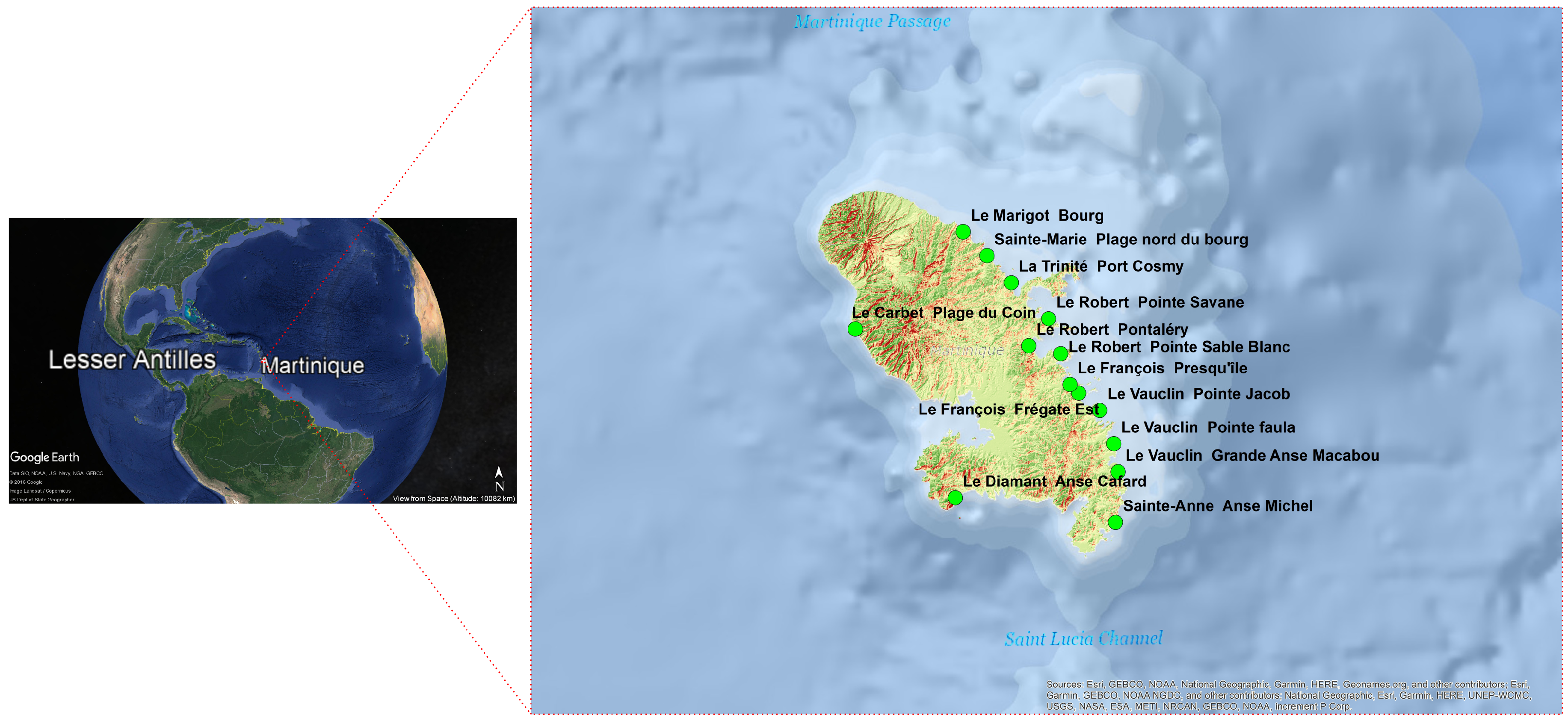
2. Study Site and Materials

The study area (Figure 1) is situated on Martinique Island, France, which is located in the Lesser Antilles arc of the Caribbean Sea. The island is characterized by a humid tropical climate and is influenced by the trade winds throughout the year, with episodic cyclones. With respect to the coastal morphology, two-thirds of the island is constituted of sandy and vegetated (mangrove) beaches, and $75\%$ of them are pocket beaches. A well-defined trend in shoreline retreat has been evaluated in the last 50 years [38]. Moreover, the above-mentioned concerns over Sargassum encroachments (Section 1.2) demand that the issue be addressed. This has led to the definition of a program for morphodynamics and algae monitoring, with the intent of implementing cost-effective, non-invasive instruments and straightforward methodologies in order to deal with the largest number of coastal sites. Therefore, a system composed of low-cost, smartphone-based cameras—SOLARCAM${}^{\copyright }$ (Marseille, France, https://www.solarcam.fr)—has been installed in Martinique, aiming at monitoring both coastal morphodynamics and beach/water quality. More generally, a station of this monitoring system is equipped with a camera, powered by a modified Sony Android smartphone, which produces time lapse in real time, a small solar panel (for charging), and a battery that supports the system’s operation even during poor weather conditions. Up to one image every minute is transmitted over 3G, and the interval is tunable, depending on the solar panel power and especially on the scopes. A plastic case hosts the phone and a laminate band is used to affix it to a support, which could be a pole, house pylon, or even a tree. Images with a resolution of 8 megapixels are promptly stored on an FTP server. The price of the described representative station (excluding the monthly 3G communication expenses) is on the order of $400$€. The configuration guarantees good portability, cheapness, simplicity in communication and installation, and optimal resolution. Drawbacks are especially linked to network signal fluctuations, low acquisition frequency, and contingent displacements due to strong winds or temperature-related material deformations of the case or support. At the time of writing, 14 coastal sites have been equipped, starting from October 2018, at both Atlantic and Caribbean Sea sides. These include harbours and sandy/vegetated beaches. Among these, six sites were chosen for validation of the classification methodology and nine sites for presenting the calibration of the beached/floating Sargassum warning system, described in Section 5. Figure 1 shows the overall Martinique territory, with the superposed equipped coastal sites, distributed along the coastal area.

The six-camera dataset is divided into two main categories, beach and harbour. The images used for this work, (totaling 160), are divided into training and testing sets, in the respective proportions of $55\%$ and $45\%$. Specifically, with respect to the beach-type category, seven classes were used, related to natural morphologies and land covers, including algae, anthropic structure, sea foam and swash, sand, sky, vegetation, and sea water. The harbour-type category does not include the sandy area, which has been found to be useless and to generate issues during the CNN retraining phase.

3. Methods for Data Processing

3.1. Sticky-Edge Adhesive Superpixels

In this work, over-segmentation processing is adopted by using sticky-edge adhesive superpixels [39]. Data fed into the input layer of CNN classification must be images with a fixed size, whereas the segmented regions generated from traditional superpixel partitioning methods vary greatly in size and shape. The selection of the superpixel algorithm and the choice of parameters greatly affect the final results of image classification. Theoretically, the selected over-segmentation algorithm favors boundary adherence and generates superpixels with high compactness. This chosen method is built on an iterative approach motivated by SLIC [24], but with superpixels snapped to the edges of the image, resulting in higher-quality boundaries. SLIC generates superpixels by clustering pixels based on the color similarity and proximity in the image plane. This algorithm performs k-means clustering in the $5D$ space of color information and pixel location, based on gradient-ascent methodology. SLIC uses the Lab color space, as it is perceptually uniform for small color distances. First, it samples k regularly spaced cluster centers. Then, each pixel in the image is attributed to the nearest cluster centre whose search area overlaps it. After assigning all pixels to cluster centers, they are updated by computing an average over the 5D vector of all pixels assigned to the cluster. This process of attributing pixels and updating centers is iteratively repeated until no new attribution occurs. Then, since the method makes use of the main image edges to snap the superpixels’ region contours, structured forests is used [39] to implement edge detection in the image. Structured forests is a very fast edge detector that achieves excellent accuracy, based on a structured learning approach [39]. The employment of this very fast edge detector increases the boundary recall of SLIC superpixels. After the first step of superpixel partitioning, the generated superpixel-level segmented regions can be classified by using high-level features extracted by CNN.

3.2. MobileNet CNN and Mechanisms of Deep Transfer Learning

Generally speaking, a CNN is a multi-layer perceptron network with many hidden convolutional layers and pooling layers [40]. It is very similar to a biological neural network. The extraction of engineered features and data recognition, necessary in the traditional artificial neural network algorithm, is avoided in CNN-type structures. This is very valuable when dealing with image processing since it is qualified in features detection including color, texture, shape, and image topology [41].

MobileNet [42], a recent CNN framework proposed by Google, is built on blocks called depthwise separable convolutions. Depthwise convolution applies a single filter to each input channel, followed by a pointwise convolution, which applies a $1\times 1$ convolution to combine the outputs. Unlike a regular convolution which filters and combines in one step, this is called separable since it splits this step into two separate steps—one for filtering and one for combining. Particularly, in the v2 architecture (MobileNet V2 [43]) the residual connections and the expand/projection layers are introduced. The pointwise convolution became a projection layer, which projects data with higher channels into a tensor with lower dimensions. This kind of layer is called a bottleneck layer since it normally decrements the amount of data that flows through the network. In the main block, an expansion layer is introduced, which expands the number of channels in the data which feed the depthwise convolution. Each layer has a batch normalization and the activation function is ReLU6 (except for the projection one). The novelty is also in the residual connections, which connect the beginning and end of convolutional blocks with skip connections. The network can access earlier activations which could be not modified in the convolutional block. This seems essential in order to build networks of great depth [44]. The full MobileNet V2 architecture consists of 17 of these building blocks in a row, followed by a regular $1\times 1$ convolution, a global average pooling layer, and a classification layer. This strategy in the convolutional blocks significantly reduces the number of parameters when compared to normal convolutions and makes the network architecture lightweight. Using these convolutions marginally sacrifices accuracy to obtain a low-complexity deep neural network, making it very suitable for mobile and embedded vision applications.

In this work, a transfer learning methodology is employed using the pre-trained CNN MobileNet-V2 architecture [43] implemented within TensorFlow-Hub [45] in order to classify coastal oblique images. As an alternative to building a model from scratch, here we explored the possibility to improve a previously trained model which had already been trained to solve a similar (larger) classification problem, specifically, on the Imagenet database [46]. It is surprisingly effective to take advantage of features learned by a bigger database [46]. So, a new final classifier is added to a pre-trained “frozen” model, and only the weights of this layer on top of the network are updated during training—a fully-connected layer that determines the image class given the set of features extracted from the convolutional base network. Contrary to training large models, less regularization and data augmentation techniques are used since small models have less trouble with overfitting [42]. CNNs require input data to be small square image regions (patches) due to the shape limitation of the network. Since the shape of superpixels is irregular, superpixels cannot be directly used as input data to feed CNNs. Therefore, the center pixel of each superpixel is selected and a square centered on the superpixel center is used as the input data. After the classification of squares, the resolving class label is assigned to the associated superpixel. The patch images based on the superpixel centers are the data used by the MobileNet classifier, and the superpixels mine the specific pixels that are labelled in the resolving classification. Hence, the center pixel plays the role of a connection between CNN and the superpixels.

3.3. Refining via Conditional Random Field

Fully connected CRF is a probabilistic graphical model [28], employed in this work to smooth raw segmentation maps (the output of CNN-based superpixel classification). Each node of the graph is assumed to be linked to every other pixel in the image. Using the Gaussian CRF potentials, the method is able to consider not only neighboring information but also long-range dependencies between pixels, and contextually the model is responsive to fast mean-field inference [29]. The model couples nodes, favoring same-label assignments to spatially proximal pixels. Qualitatively, the primary function of these long-range CRFs is to clean up the spurious predictions of weak classifiers built on top of the CNN. The combination of CNN and CRF is of course not new [47]. The approach applied here treats every pixel as a CRF node receiving unary potentials from the CNN. The model involves the use of an energy function to minimize:

$$E(x)=\sum _i{\theta }_i(x_i)+\sum _{ij}{\theta }_{ij}(x_i,x_j),$$

(1)

where x is the label assignment for pixels from the CNN. The unary potentials explain the data cost. They are described by ${\theta }_i\left(x_i\right)=-logP\left(x_i\right)$, where $P\left(x_i\right)$ is the label probability at pixel i (i.e., as assigned by the CNN). The pairwise potentials, the second term of Equation (1), motivate the smoothness cost. They have a form that allows for efficient inference while using a fully connected graph, that is, when connecting all pairs of image pixels, i,j [29]. According to the original work in [28], the pairwise potential is defined as:

$${\theta }_{ij}(x_i,x_j)=\mu (x_i,x_j)[{\omega }_{1}exp(-\frac{|p_i-p_j{|}^2}{2{\sigma }_{\alpha }^2}-\frac{|I_i-I_j{|}^2}{2{\sigma }_{\beta }^2})+{\omega }_{2}exp(-\frac{|p_i-p_j{|}^2}{2{\sigma }_{\gamma }^2})],$$

(2)

where $\mu (x_i,x_j)$, referred to as the label compatibility function, is assigned equal to 1 if $x_i\ne x_j$ and 0 otherwise, which means that only nodes with different labels can be penalized. The expression describes two Gaussian kernels in different feature spaces, referred to as pixel compatibility function. The first, “bilateral” kernel depends on both pixel positions (identified as p) and colors (Lab space, denoted as I), and the second kernel only depends on pixel positions. The hyperparameters ${\sigma }_{\alpha }$, ${\sigma }_{\beta }$, ${\sigma }_{\gamma }$ mainly control the scale of Gaussian kernels. The first kernel constrains pixels having similar color and position to gain similar labels, while the second kernel merely considers proximity in space when enforcing smoothness [29]. The kernel parameters ${\omega }_{\left(n\right)}$ are equally weighted, and both set to 1. In particular, high-dimensional filtering algorithms [28] significantly speed up the computation, resulting in an algorithm that is quick in practice.

3.4. Workflow of STICKY-CNN-CRF Classification

The workflow of the superpixel-based CNN classification is shown in Figure 2, which includes two main phases—training and testing, including the application of the semantic segmentation. Firstly, by sticky-edge adhesive superpixels partitioning, the original SolarCam images from the training data are over-segmented into several regions, which are used as the spatial processing units for CNN classification. The image is manually labelled by following a modified methodology from [18]. Next, transfer learning enables the retraining of the experimental network, based on MobileNet V2 convolutional neural network, described in Section 3.4. The samples of labelled regions are used to retrain the CNN parameters, based on resolving the accuracy of the classification. The patch size used is equal to 96 pixel square. Finally, with regard to the semantic segmentation phase, the testing dataset from the original images are firstly over-segmented by means of the sticky-edge adhesive algorithm. The superpixel patches are classified using the pre-trained network. Then, the fully-connected CRF is applied for smoothing the results and better capturing the boundaries of the regions.

SolarCam images are used for superpixel partitioning, CNN training, superpixel-based classification with CNN, and finally refining via fully-connected CRF.

As an example, for the explanation of the main steps related to the semantic segmentation phase, Figure 3 shows the original image, over-segmented in superpixels (Figure 3a,d), the CNN-based superpixels classification with class labels as mentioned above (Figure 3b,e), and finally the result from the CRF refining mechanism used to smooth the segmentation map (Figure 3c,f).

4. Results

In this section, the performance of the method described in Section 3 is evaluated on the basis of 72 images in the testing dataset, based on six Solarcam cameras (12 images per camera), with full resolution of 3264 × 2448 pixels. Around 3000 superpixels for each image were used as processing units for CNN training.

The metric used in this work for analyzing the performance of the methodology presented is mainly based on a confusion matrix, a table with rows and columns reporting the number of false positives ($FP$), false negatives ($FN$), true positives ($TP$), and true negatives ($TN$), which allows for more detailed analysis than the mere proportion of correct classifications (accuracy). “True” or “false” indicates if the classifier predicted the class correctly, whereas “positive” and “negative” indicate if the classifier predicted the desired class. The way to summarize the table is here presented as a function of the $F1$-$score$, which is defined as an equal mean of Precision and $Recall$. The $Precision$ score is based on the total number correctly classified as positive divided by the total number of predicted positives: $Precision=\frac{TP}{TP+FP}$. The Recall explains the total number of correctly classified positives divided by the total number of positives: $Recall=\frac{TP}{TP+FN}$. Furthermore, the sensitivity of results on the superpixels and CRF hyperparameters were assessed to demonstrate the capabilities and applications of the trained model.

4.1. Experimental Results

During the CNN transfer training procedure, the main hyperparameters were kept constant: the learning rate at 0.01, the training steps fixed as 2000. The batch size of the SolarCam classification datasets of coastal images was set to 100. The codes ran on a computer with Intel^® Core${}^{\mathrm{TM}}$ i5-7300HQ CPU @ 2.50 GHz, 16 GB RAM, and Python 3.7. The gradient was computed via batch gradient descent, employing only the CPU. TensorFlow [48] was chosen as the deep learning platform. Two models were trained, related to the categories mentioned above (i.e., beach morphology and harbour-type land cover). The classification accuracy was evaluated with respect to the superpixel-based CNN classification, and then by inspecting the pixel-scale results, following CRF refinement.

Table 1. Summary of superpixel-based CNN classification accuracy ($F1$-$score$), for both categories investigated: beach morphology and harbour-type land cover, respectively. Image classes were analyzed singularly. The number of training and testing superpixel patches are highlighted.

		Beach			Harbour
Classes	$\mathit{F}\mathbf{1}$-$\mathit{Score}$	Training Superpixels	Testing Superpixels	$\mathit{F}\mathbf{1}$-$\mathit{Score}$	Training Superpixels	Testing Superpixels
Algae	0.88	11,727	10,128	0.85	14,739	13201
Anthro-road	0.85	339	521	0.83	2319	1563
Foam-swash	0.88	11,814	16,230	0.93	13,026	230,217
Sand	0.91	6864	4260	-	-	-
Sky	0.84	1482	852	0.96	1838	1803
Vegetation	0.89	53,676	59,426	0.87	58,321	62,032
Water	0.95	32,679	25,362	0.93	26,449	15,260

summarizes the CNN prediction accuracies ($F1$-$score$) at superpixel scale. The number of training and testing superpixels was similar since the number of images used for training and testing were almost equal. The overall classification accuracy was very positive. The maximum ($96\%$) was reached by the sky class, related to the harbour-type category, which was trained with the smaller amount of data, while the minimum was associated to the anthropic one, among both categories. Indeed, anthropic regions are often too small and difficult to detect, in both conditions. Conversely, the sky class for the beach-type category was not well predicted. It was also found that the presence of kites (Figure A1 in the Appendix A) could have invalidated the results. The algae were quite well predicted for both categories. (See Figure A1 and Figure A2 in the Appendix A for further qualitative results).

In Figure 4, the confusion matrices describing the classification accuracies, at pixel-scale, after CNN classification and CRF detailing, are shown as normalized data per class and category under analysis. Further elucidations about the main metrics used are presented in

Table 2. Summary of results by using metrics: precision, recall, and $F1$-$score$, for both categories investigated: beach morphology and harbour-type land cover, respectively. Image classes were analyzed singularly.

		Beach			Harbour
Classes	$\mathit{Precision}$	$\mathit{Recall}$	$\mathit{F}\mathbf{1}$-$\mathit{Score}$	$\mathit{Precision}$	$\mathit{Recall}$	$\mathit{F}\mathbf{1}$-$\mathit{Score}$
Algae	0.95	0.85	0.90	0.82	0.81	0.80
Anthro-road	0.95	0.65	0.77	0.72	0.8	0.75
Foam-swash	0.97	0.83	0.89	0.78	0.84	0.81
Sand	0.80	0.89	0.84	-	-	-
Sky	0.97	0.96	0.97	0.99	0.86	0.93
Vegetation	0.72	0.94	0.82	0.81	0.7	0.75
Water	0.78	0.93	0.85	0.81	0.88	0.85

. With respect to beach morphology, the range of classification $F1$-$score$ was between $77\%$ and $96\%$. The anthropic-road class reached the minimum, while the sky the maximum recall. The vegetation and anthropic-road classes had higher incorrect classifications, where a peak of $26\%$ of FP for the vegetation class was evident. The algorithm was surprisingly able to predict beached algae well, with a $85\%$. As excepted, misclassification derived from recognition ambiguities with respect to spatially closer classes, particularly vegetation and sand. The foam and swash areas were combined in a unique class, considering their highly similar visual appearance and since this type of neural network has no contextual information capability. Together with the water class, they were well predicted. In the analysis of the confusion matrix related to the harbour-type category, the results appeared slightly sparse. The classification $F1$-$score$ was in the range of $75\%$ to $93\%$. There was often confusion between vegetation and algae classes. This should be explained because these two class types may have similar spectral features. For both categories, it is evident that the vegetation class was well predicted (high recall), but most often the buildings, which cover very tiny areas of the images, were not well recognized by the CNN classification algorithm. The path size of the CNN network plays a fundamental role in this issue since it was found that superpixels less than almost two-thirds of the path size of the CNN network (96 pixels) are not able to catch the deep features.

As is well known, the overall accuracy is mainly influenced by the dominant classes in an image. A sort of salt-and-pepper effect was found at very small-scale classifications, especially for algae regions, labelled as vegetation.

See Figure A1 and Figure A2 in the Appendix A for further (qualitative) results.

4.2. Parameter Sensitivity Analysis

This paper presents a CNN-based classification method for coastal image analysis using superpixel over-segmentation and CRF refining. The following section discusses the influences of the superpixel over-segmentation input for CNN-based classification and the CRF hyperparameters, and the effects of both on the pixel-scale results.

Figure 5 shows a sensitivity analysis carried out for the evaluation of the impact of the number of superpixels used for image partitioning on the final accuracy, in which results are divided into each class studied. A higher slope was observed in the range between 20 and 200 superpixels, with respect to the right part of the curve. Approximately 850 superpixels were needed to roughly cover the patch size of 96 pixels used as the CNN processing unit, using images having 8 Mp resolution as the case study. It is clear that for almost all the classes, before reaching this value, convergence at the higher score was achieved, even if a kind of oscillation was still present, mostly attributable to the influence of CRF in the final segmentation. In order to find a compromise between computation speed and efficiency, the number of superpixel units for CNN processing in the evaluation procedure was set to 800. We also investigated the eventual influence of the compactness index in superpixel generation. This index indicates the ratio of minimum enclosing rectangle area of the superpixel to the number of pixels contained within it. After some experiments, by applying values around the default one, no specific correlation was found.

On the basis of the above analysis, it can be summarized that there was a clear scale effect in the final classification accuracy. This was particularly true in the regions with high complexity (e.g., algae). That is, the deep features appeared less valuable at large scales as there was major variability and lower consistency. There is no definite evidence to suggest that there is a unique superpixel scale for all optimal classifications in each class.

The refinement step of semantic segmentation employs fully connected CRFs, which makes use of the superpixels labelled regions as unary potentials and pairwise potential terms, modeling each pair of pixels i and j in the image, no matter how far from each other they lie. The “scale” of the Gaussian kernels, which shapes the pairwise potential, is controlled by the hyperparameters (see Section 3), which significantly influence the final semantic segmentation map. By fixing the values of ${\omega }_2=1$ and ${\omega }_1=1$, the best combinations of the mentioned parameters were sought by exploring the solution space on a subset of the testing sample (50 images). In the literature, challenging searching solutions are employed based on schemes such as the coarse-to-fine search [47] or structured output SVM [49]. In this context, a calibration exercise was considered in order to estimate the optimal range of values useful for optimizing the pixel-wise classification (F1-score) accuracy. We fixed the number of mean-field iterations at 20 for the entire analysis. Furthermore, since the running time is highly influenced by the choice of the image scale, this value was fixed to $0.5$, ensuring computation efficiency. Figure 6 maps the $F1$-$score$, averaged among all the classes and the two categories under analysis, in the space of the hyper-parameters ${\sigma }_{\alpha },{\sigma }_{\gamma },{\sigma }_{\beta }$. The range of values investigated was chosen considering the work in [47]. Specifically, the ranges were ${\sigma }_{\beta }\in [2:12]$, ${\sigma }_{\alpha }\in [20:120]$, and ${\sigma }_{\gamma }\in [30:220]$.

A large range of values which led to solutions having accuracies greater than $70\%$ was found for kernel hyperparameters ${\sigma }_{\alpha }$ and ${\sigma }_{\gamma }$, while a smaller amplitude of admissible values was related to ${\sigma }_{\gamma }$. To some extent, the former models the standard deviations for the location component of the color-dependent and color-independent kernels. The latter is related to the standard deviation for the color component of the color-dependent term, and it appeared to have a much greater impact on the acceptable accuracy. The values chosen for use in the evaluation phase presented above were ${\sigma }_{\alpha }=90,{\sigma }_{\gamma }=130,{\sigma }_{\beta }=5$.

Finally, as regards the superpixels image partitioning, a newly proposed and widely used algorithm, SEEDS [50], was also briefly tested in order to compare its influence on the feature extraction and final superpixel classification results with respect to the sticky-edge algorithm. The running time decreased by a factor of 1.8. With regard to the overall dataset, the superpixel classification ($F1$-$score$) achieved slightly lower ($2.64\%$) accuracy for the final classification, obtained by averaging all types of classes. It can be concluded that sticky-edge adhesive algorithm performed slightly better than SEEDS with almost the same running time, but with benefits from the shapes of superpixel regions. The main reason is related to the fact that sticky-edge generates superpixel regions whose boundaries, derived from an edge detector, are closer to practical land cover regions. Conversely, superpixel regions generated by SEEDS could cross the border of two land covers, especially for those with blurred borders. Moreover, the non-uniformity in the size and shape of superpixel regions, more noticeable in SLIC, is supposed to improve the generalization capability of CNN, which could prevent over-fitting.

5. Discussion

At present, the great availability of low-cost camera systems and the great potential of portable devices, coupled with autonomous and efficient energy collectors (e.g., solar panel), push the limits of the current approaches for coastal video monitoring. Moreover, the newest advances in machine learning allow further investigation of the capabilities for image understanding. In many occasions, environmental contingencies require these types of new methodologies and tools to be easily deployable and maintainable.

Specifically, in order to face the Sargassum emergency in the Lesser Antilles and to benefit from these new methods and instruments, a warning framework has been implemented in Martinique that is useful for the quantification of floating and beached algae. The Sargassum warning framework deployed uses the two phases described in Section 3. It makes use of the models trained and presented above (two more models were trained) for employing an automatic segmentation in quasi-real-time. Presently, the SolarCam stations in Martinique collect image snapshots every hour. Every three daylight hours, starting from 09:00 a.m., an automatic routine is launched which performs an automatic image segmentation. In this scenario, a region of interest (ROI) oriented toward the field-of-view (FoV) areas prospectively affected by the beached/floating algae is considered. This allows high computation power and time during CNN classification to be avoided. The predicted classes are analyzed for the extraction of the Sargassum blobs. These potential predicted blobs are filtered based on relative euclidean distances to the other predicted classes (specifically sand, foam, terrain/vegetation, and sky, respectively) in order to remove suspected outliers (mainly false positives). Subsequently, the computation of boundaries and areas of each spot is given. Finally, the determination of an expected warning is based on site-specific temporal thresholds. Geo-referenced data are being used, where available, to report data in meters rather than pixels, by means of a standard method for georectification [51]. A location map where the framework is being tested is shown in Figure 7. With respect to all sites monitored, presented in Section 2 (shown as points), the map marks the warning system stations in red and green. Specifically, the green and red colors indicate the percentage of manually validated data with respect to the excluded ones, respectively. This means that a percentage is affected by different issues, mainly related to acquisition problems, loss of data, blurred conditions (i.e., the two sites facing the Caribbean Sea), foggy environment, or classification errors.

In the same Figure 7, time series of floating/beached Sargassum for a few sites as examples are drawn on top of the map. The red lines represent the temporal evolutions of the pixel/real-world areas computed every 3 h (red points) at each station, while the shaded red curves on top of the red lines, referred to as the “holes uncertainties”, are computed as tiny regions inside the great algae spots, which are perceived as questionable predictions.

As mentioned above, at each site under analysis, the definition of a double threshold is being realized, strictly related to spatial and temporal constraints. Particularly, as an example with respect to the beach-type category, a first absolute minimum threshold was defined, specified as a percentage of the beach covered area ($30\%$). Furthermore, in order to ensure reliable information in the event of beaching/arrival, so as to avoid the dissemination of useless warnings (i.e., false positives), the image under analysis should exhibit a computed Sargassum area greater than $20\%$ of the prior temporal result. The warning framework is still under validation in order to be available for communities/municipalities.

The regions predicted as algae were seen to be affected by inaccuracies, specifically inside the great blobs regions or at the boundaries, which are referred to as the questionable predictions above. The CRF algorithm adopted, based on a fully connected graph [28], captures long-range dependencies between image pixels. It is used to detail the CNN raw classification and to reclassify pixel labels. Its hyperparameters combination, which controls the “scale” of Gaussian kernels, was calibrated on several images with almost distinctive conditions (Section 4), but it still suffered from the aforementioned ambiguities. A straightforward way to improve the semantic segmentation output was conceived and built, based on the inclusion of the effects of boundary detection by re-employing an edge-adhesive superpixels map. So, it was surprising to investigate the dual task of the effects of superpixels on the semantic segmentation. A great interest of the coastal image community is related to the identification of the so-called precise semantic boundaries (e.g., shoreline, vegetation limit), which requires not only the detection of several boundaries but the association of semantic classes to them. In the literature, this idea is typically seen as a combination of boundary detection and semantic segmentation [52], which requires an association of precise boundaries to a semantic class related to them. A common approach to the task is to separate methods such as semantic segmentation and contour detection, and hence fuse the results of both steps. In this work, a superpixel over-segmentation was performed by employing a great number of superpixels (i.e., 50,000), allowing a further refinement and smoothing of the boundaries. So, the semantic segmentation CRF output was snapped to the superpixels by majority voting of the regions. This means that superpixels that overlapped more than $50\%$ with the semantic class were assigned the corresponding label. Figure 8 shows an example of the result from the implementation of this further refinement. At the bottom, it highlights two magnifications extracted from a zoom-box, defined in Figure 8b. The CRF output (Figure 8c) from the methodology in Section 3 was further refined by means of the superpixels and the majority voting of the regions (Figure 8d). Particularly, it is evident that the sparse small regions labelled as water or vegetation were re-classified with the classes of the superpixels which incorporated them (mainly algae, vegetation). Moreover, it allowed a smoothing much more adherent to the reality (interfaces of water–sand or algae–sand). Particularly relevant for improving Sargassum classification, we observed an increase in classification accuracy. On the basis of 20 images from the same testing database, as above, the $F1$-$score$ increased by $2.3\%$ compared to the results discussed in Section 4 with respect to beach-type morphology.

The great advantage of employing such models could be straightforward for several applications related to coastal monitoring research and case studies. Because only a few images are required for training since the superpixel partitioning creates a broad and adequate database for CNN transfer learning (i.e., the number of training superpixels in Table 1), easy prototyping of models can be realized. Applications related to shoreline detections and/or nearshore bars evolution, beach widths, dune growth, or Posidonia banquettes dynamics [53] could result in effortless automation. With respect to coastal classification algorithms (e.g., based on SVM [16]), the transfer learning method described here allowed us to employ $10\times$ less ground-truth data while still achieving around the same classification accuracy [16]. Furthermore, the powerful refining capability of the fully connected CRF makes it possible to better catch classes’ borders and small scattered data, with respect to the superpixel scale [16].

There are still some limitations to the proposed approach, most significantly the disadvantage related to unstable plastic support of the SolarCam. This causes the cameras to experience high-frequency vibrations due to low-to-average winds, and, in a few occasions, minor absolute displacements due to wind gusts. The latter condition is very inconvenient due to loss of image geometry reference, which is useful for the real-world computation of Sargassum area. Additionally, problems of variations in lighting and weather change greatly affect distributions of color, contrast, and brightness. Herein we observed, particularly during season transitions, certain soil cover appearance changes (vegetation became reddish) and this could greatly affect the classification efficacy. Another practical limitation is due to issues in proper network coverage.

6. Conclusions

This work combines ideas from per-superpixel deep convolutional neural networks and fully connected CRF, creating a method able to generate semantically accurate predictions and detailed segmentation maps, while remaining computationally efficient. To achieve a high overall classification accuracy, the over-segmentation has to hold a balance between compactness and boundary accuracy. Accordingly, an algorithm based on SLIC specifically focused on snapping the boundaries, computed by means of a fast and effective edge detector, is employed. The work demonstrates the general effectiveness of a small, very fast, existing CNN framework (MobileNetV2) for image patch classification. The fully connected CRF was proved to be very efficient in detailing a sparse and raw semantic segmentation. Experimental results indicate that for beach and harbour-type image categories the average accuracies were in the range of $75\%$ to $96\%$, across a dataset derived from six cameras. By means of a superpixel over-segmentation method at a variety of scales, in coastal-specific environments, the effectiveness of deep features extracted by CNN was evaluated and the optimal scale was discussed. A sensitivity of final classification accuracy to the CRF hyperparameters space is proposed. For some images with few small land-cover spots or some simple artificial regions, the methodology can suffer from ambiguities. A case study related to the implementation of a warning system for Sargassum monitoring is presented to exhibit the capabilities and potential applications of the trained models. Particularly, when a further post-processing procedure based on superpixels region-based majority voting was applied, the $F1$-$score$ related to the Sargassum class reached $91\%$, with respect to images of beach-type morphology.

The presented procedure promotes the use of camera-based images for applications related to automatic feature recognition and coastal quality monitoring. Further experiments are being planned with a larger dataset (including other Lesser Antilles islands) and aiming at the application of the method to other sources of data, such as videos. Moreover, further studies are focused on processing the time-series data derived from the warning system in order to retrieve parametrization of the meteo-oceanographic forces useful for describing the probability of occurrence of algae degradation over time, disintegration due to wave impact, or removal due to tide oscillations.

References

1. Osorio, A.F.; Montoya-Vargas, S.; Cartagena, C.A.; Espinosa, J.; Orfila, A.; Winter, C. Virtual BUOY: A video-based approach for measuring near-shore wave peak period. Comput. Geosci. 2019, 133, 104302. [Google Scholar] [CrossRef]
2. Almar, R.; Blenkinsopp, C.; Almeida, L.P.; Cienfuegos, R.; Catalán, P.A. Wave runup video motion detection using the Radon Transform. Coast. Eng. 2017, 130, 46–51. [Google Scholar] [CrossRef]
3. Ibaceta, R.; Almar, R.; Catalán, P.A.; Blenkinsopp, C.E.; Almeida, L.P.; Cienfuegos, R. Assessing the performance of a low-cost method for video-monitoring the water surface and bed level in the swash zone of natural beaches. Remote. Sens. 2018, 10, 49. [Google Scholar] [CrossRef] [Green Version]
4. Andriolo, U. Nearshore Wave Transformation Domains from Video Imagery. J. Mar. Sci. Eng. 2019, 7, 186. [Google Scholar] [CrossRef] [Green Version]
5. Bergsma, E.W.; Conley, D.C.; Davidson, M.A.; O’Hare, T.J. Video-based nearshore bathymetry estimation in macro-tidal environments. Mar. Geol. 2016, 374, 31–41. [Google Scholar] [CrossRef] [Green Version]
6. Valentini, N.; Saponieri, A.; Damiani, L. A new video monitoring system in support of Coastal Zone Management at Apulia Region, Italy. Ocean. Coast. Manag. 2017, 142, 122–135. [Google Scholar] [CrossRef]
7. Ondoa, G.A.; Almar, R.; Castelle, B.; Testut, L.; Léger, F.; Sohou, Z.; Bonou, F.; Bergsma, E.W.J.; Meyssignac, B.; Larson, M. Sea Level at the Coast from Video-Sensed Waves: Comparison to Tidal Gauges and Satellite Altimetry. J. Atmos. Ocean. Technol. 2019, 36, 1591–1603. [Google Scholar] [CrossRef]
8. Díaz-Gil, C.; Smee, S.L.; Cotgrove, L.; Follana-Berná, G.; Hinz, H.; Marti-Puig, P.; Grau, A.; Palmer, M.; Catalán, I.A. Using stereoscopic video cameras to evaluate seagrass meadows nursery function in the Mediterranean. Mar. Biol. 2017, 164, 137. [Google Scholar] [CrossRef]
9. Beliaeff, B.; Pelletier, D. A general framework for indicator design and use with application to the assessment of coastal water quality and marine protected area management. Ocean. Coast. Manag. 2011, 54, 84–92. [Google Scholar] [CrossRef] [Green Version]
10. Bracs, M.A.; Turner, I.L.; Splinter, K.D.; Short, A.D.; Lane, C.; Davidson, M.A.; Goodwin, I.D.; Pritchard, T.; Cameron, D. Evaluation of Opportunistic Shoreline Monitoring Capability Utilizing Existing “Surfcam” Infrastructure. J. Coast. Res. 2016, 319, 542–554. [Google Scholar] [CrossRef]
11. Harley, M.D.; Kinsela, M.A.; Sánchez-García, E.; Vos, K. Shoreline change mapping using crowd-sourced smartphone images. Coast. Eng. 2019, 150, 175–189. [Google Scholar] [CrossRef]
12. Andriolo, U.; Sánchez-García, E.; Taborda, R.; Andriolo, U.; Sánchez-García, E.; Taborda, R. Operational Use of Surfcam Online Streaming Images for Coastal Morphodynamic Studies. Remote. Sens. 2019, 11, 78. [Google Scholar] [CrossRef] [Green Version]
13. Quartel, S.; Addink, E.A.; Ruessink, B.G. Object-oriented extraction of beach morphology from video images. Int. J. Appl. Earth Obs. Geoinf. 2006, 8, 256–269. [Google Scholar] [CrossRef]
14. Valentini, N.; Saponieri, A.; Molfetta, M.G.; Damiani, L. New algorithms for shoreline monitoring from coastal video systems. Earth Sci. Inform. 2017, 10, 495–506. [Google Scholar] [CrossRef]
15. Aarninkhof, S.G.; Turner, I.L.; Dronkers, T.D.; Caljouw, M.; Nipius, L. A video-based technique for mapping intertidal beach bathymetry. Coast. Eng. 2003, 49, 275–289. [Google Scholar] [CrossRef]
16. Hoonhout, B.M.; Radermacher, M.; Baart, F.; van der Maaten, L.J. An automated method for semantic classification of regions in coastal images. Coast. Eng. 2015, 105, 1–12. [Google Scholar] [CrossRef] [Green Version]
17. Othman, E.; Bazi, Y.; Alajlan, N.; Alhichri, H.; Melgani, F. Using convolutional features and a sparse autoencoder for land-use scene classification. Int. J. Remote Sens. 2016, 2149–2167. [Google Scholar] [CrossRef]
18. Buscombe, D.; Ritchie, A. Landscape Classification with Deep Neural Networks. Geosciences 2018, 8, 244. [Google Scholar] [CrossRef] [Green Version]
19. Chen, Y.; Ming, D.; Lv, X. Superpixel based land cover classification of VHR satellite image combining multi-scale CNN and scale parameter estimation. Earth Sci. Informatics 2019, 12, 341–363. [Google Scholar] [CrossRef]
20. Long, J.; Shelhamer, E.; Darrell, T. Fully convolutional networks for semantic segmentation. In Proceedings of the IEEE Conference on Computer Vision and Pattern Recognition, Boston, MA, USA, 7–12 June 2015; pp. 3431–3440. [Google Scholar]
21. Aggarwal, C.C. Data Classification: Algorithms and Applications; CRC Press: Boca Raton, FL, USA, 2014. [Google Scholar]
22. Roy, P.; Ghosh, S.; Bhattacharya, S.; Pal, U. Effects of degradations on deep neural network architectures. arXiv 2018, arXiv:1807.10108. [Google Scholar]
23. Wang, M.; Liu, X.; Gao, Y.; Ma, X.; Soomro, N.Q. Superpixel segmentation: A benchmark. Signal Process. Image Commun. 2017, 56, 28–39. [Google Scholar] [CrossRef]
24. Achanta, R.; Shaji, A.; Smith, K.; Lucchi, A.; Fua, P.; Süsstrunk, S. SLIC superpixels compared to state-of-the-art superpixel methods. IEEE Trans. Pattern Anal. Mach. Intell. 2012, 34, 2274–2282. [Google Scholar] [CrossRef] [PubMed] [Green Version]
25. Lv, X.; Ming, D.; Chen, Y.Y.; Wang, M. Very high resolution remote sensing image classification with SEEDS-CNN and scale effect analysis for superpixel CNN classification. Int. J. Remote. Sens. 2019, 506–531. [Google Scholar] [CrossRef]
26. Chen, L.C.; Barron, J.T.; Papandreou, G.; Murphy, K.; Yuille, A.L. Semantic image segmentation with task-specific edge detection using CNNs and a discriminatively trained domain transform. In Proceedings of the IEEE Computer Society Conference on Computer Vision and Pattern Recognition, Las Vegas, NV, USA, 26 June–1 July 2016. [Google Scholar] [CrossRef] [Green Version]
27. Marmanis, D.; Schindler, K.; Wegner, J.D.; Galliani, S.; Datcu, M.; Stilla, U. Classification with an edge: Improving semantic image segmentation with boundary detection. Isprs J. Photogramm. Remote. Sens. 2018, 135, 158–172. [Google Scholar] [CrossRef] [Green Version]
28. Krähenbühl, P.; Koltun, V. Efficient inference in fully connected crfs with Gaussian edge potentials. In Proceedings of the Advances in Neural Information Processing Systems 24: 25th Annual Conference on Neural Information Processing Systems 2011 (NIPS 2011), Granada, Spain, 12–15 December 2011. [Google Scholar]
29. Chen, L.C.; Papandreou, G.; Kokkinos, I.; Murphy, K.; Yuille, A.L. DeepLab: Semantic Image Segmentation with Deep Convolutional Nets, Atrous Convolution, and Fully Connected CRFs. IEEE Trans. Pattern Anal. Mach. Intell. 2018, 40, 834–848. [Google Scholar] [CrossRef]
30. Stumpf, R.P. Applications of satellite ocean color sensors for monitoring and predicting harmful algal blooms. Hum. Ecol. Risk Assess. Int. J. 2001, 7, 1363–1368. [Google Scholar] [CrossRef]
31. Wang, M.; Hu, C. Mapping and quantifying Sargassum distribution and coverage in the Central West Atlantic using MODIS observations. Remote Sens. Environ. 2016, 183, 350–367. [Google Scholar] [CrossRef]
32. Gower, J.; Young, E.; King, S. Satellite images suggest a new Sargassum source region in 2011. Remote Sens. Lett. 2013, 764–773. [Google Scholar] [CrossRef]
33. Louime, C.; Fortune, J.; Gervais, G. Sargassum Invasion of Coastal Environments: A Growing Concern. Am. J. Environ. Sci. 2017, 13, 58–64. [Google Scholar] [CrossRef] [Green Version]
34. Hu, C. A novel ocean color index to detect floating algae in the global oceans. Remote Sens. Environ. 2009, 113, 2118–2129. [Google Scholar] [CrossRef]
35. Maréchal, J.P.; Hellio, C.; Hu, C. A simple, fast, and reliable method to predict Sargassum washing ashore in the Lesser Antilles. Remote Sens. Appl. Soc. Environ. 2017, 5, 54–63. [Google Scholar] [CrossRef]
36. Wang, M.; Hu, C. Predicting Sargassum blooms in the Caribbean Sea from MODIS observations. Geophys. Res. Lett. 2017, 44, 3265–3273. [Google Scholar] [CrossRef]
37. Cox, S., H.O.; McConney, P. Summary Report on the Review of Draft National Sargassum Plans for Four Countries Eastern Caribbean; Report Prepared for the Climate Change Adaptation in the Eastern Caribbean Fisheries Sector (CC4FISH) Project of the Food and Agriculture Organization (FAO) and the Global Environment Facility (GEF); Centre for Resource Management and Environmental Studies, University of the West Indies: Cave Hill Campus, Barbados, 2019; p. 20. [Google Scholar]
38. Nachbaur, A.; Balouin, Y.; Nicolae Lerma, A.; Douris, L.; Pedreros, R. Définition des cellules sédimentaires du littoral martiniquais; Technical Report, Rapport final; BRGM/RP-64499-FR; Orleans, France, 2015. [Google Scholar]
39. Dollar, P.; Zitnick, C.L. Fast Edge Detection Using Structured Forests. IEEE Trans. Pattern Anal. Mach. Intell. 2015, 37, 1558–1570. [Google Scholar] [CrossRef] [PubMed] [Green Version]
40. Krizhevsky, A.; Sutskever, I.; Hinton, G.E. Imagenet classification with deep convolutional neural networks. Adv. Neural Inf. Process. Syst. 2012, 1097–1105. [Google Scholar] [CrossRef]
41. Zhang, J.; Marszałek, M.; Lazebnik, S.; Schmid, C. Local features and kernels for classification of texture and object categories: A comprehensive study. Int. J. Comput. Vis. 2007, 73, 213–238. [Google Scholar] [CrossRef] [Green Version]
42. Howard, A.G.; Zhu, M.; Chen, B.; Kalenichenko, D.; Wang, W.; Weyand, T.; Andreetto, M.; Adam, H. MobileNets: Efficient Convolutional Neural Networks for Mobile Vision Applications. arXiv 2017, arXiv:1704.04861. [Google Scholar]
43. Sandler, M.; Howard, A.; Zhu, M.; Zhmoginov, A.; Chen, L.C. MobileNetV2: Inverted Residuals and Linear Bottlenecks. arXiv 2018, arXiv:1801.04381. [Google Scholar]
44. He, K.; Zhang, X.; Ren, S.; Sun, J. Deep Residual Learning for Image Recognition. arXiv 2015, arXiv:1512.03385. [Google Scholar]
45. Nelli, F. Deep Learning with TensorFlow. In Python Data Analytics; Springer: Cham, Switzerland, 2018. [Google Scholar] [CrossRef]
46. Deng, J.; Dong, W.; Socher, R.; Li, L.-J.; Li, K.; Li, F.-F. ImageNet: A large-scale hierarchical image database. In Proceedings of the IEEE Conference on Computer Vision and Pattern Recognition, Miami, FL, USA, 20–25 June 2009. [Google Scholar] [CrossRef] [Green Version]
47. Chen, L.C.; Papandreou, G.; Murphy, K.; Yuille, A.L. Semantic Image Segmentation With Deep Con-Volutional Nets and Fully Connected CRFs. In Proceedings of the International Conference on Learning Representations, Banff, AB, Canada, 14–16 April 2015. [Google Scholar]
48. Abadi, M.; Agarwal, A.; Barham, P.; Brevdo, E.; Chen, Z.; Citro, C.; Corrado, G.S.; Davis, A.; Dean, J.; Devin, M.; et al. TensorFlow: Large-Scale Machine Learning on Heterogeneous Systems. Software. 2015. Available online: https://www.tensorflow.org (accessed on 23 December 2019).
49. Orlando, J.I.; Blaschko, M. Learning fully-connected CRFs for blood vessel segmentation in retinal images. Med. Image Comput. Comput. Assist. Interv. 2014, 17 Pt 1, 634–641. [Google Scholar] [CrossRef] [Green Version]
50. Van den Bergh, M.; Boix, X.; Roig, G.; Van Gool, L. SEEDS: Superpixels Extracted Via Energy-Driven Sampling. Int. J. Comput. Vis. 2015, 111, 298–314. [Google Scholar] [CrossRef]
51. Holman, R.A.; Stanley, J. The history and technical capabilities of Argus. Coast. Eng. 2007, 6, 477–491. [Google Scholar] [CrossRef]
52. Hariharan, B.; Arbeláez, P.; Bourdev, L.; Maji, S.; Malik, J. Semantic contours from inverse detectors. In Proceedings of the 2011 International Conference on Computer Vision, Barcelona, Spain, 6–13 November 2011; pp. 991–998. [Google Scholar]
53. Valentini, N.; Balouin, Y.; Laigre, T.; Bouvier, C.; Belon, R.; Saponieri, A. Investigation on the capabilities of low-cost and smartphone-based coastal imagery for deriving coastal state video indicators: Applications on the upper mediterranean. Coast. Sediments 2019, 2635–2648. [Google Scholar] [CrossRef]
Figure 1. Martinique Island, Lesser Antilles: Distribution of the coastal sites where the Solarcam system has been deployed.
Jmse 08 00023 g001
Figure 2. Workflow of the methodology: training phase useful for building the models by means of convolutional neural network (CNN) transfer learning mechanism, by using superpixel-based patches and the semantic segmentation phase, whose results are used for testing the pixel-scale classification accuracy. DCNN: deep CNN.
Jmse 08 00023 g002
Figure 3. Examples of the three steps aiming at image semantic segmentation applied to two images, representative of the two main categories analyzed, beach morphology and harbour-type cover, left and right side, respectively. (a,d) Superpixel partitioning by the sticky-edge adhesive algorithm; (b,e) CNN superpixel classification; (c,f) The final semantic segmentation by means of fully connected CRF refinement of the CNN classification.
Jmse 08 00023 g003
Figure 4. CNN + CRF pixel-scale classification results. The ground-truth data are represented on the y-axis, the predicted ones on the x-axis. The lateral bar maps the percentage of data classified. (a) The beach category of the testing database; (b) The harbour-type category.
Jmse 08 00023 g004
Figure 5. The sensitivity of the final accuracy ( F 1 - s c o r e ), from CNN-based superpixels classification and CRF refinement results at the superpixel scale.
Jmse 08 00023 g005
Figure 6. Classification sensitivity on the fully-connected CRF hyperparameters. The σ α and σ β scales, the so-called bilateral appearance kernel, depend on the pixel positions and color, respectively. σ γ scales the Gaussian kernel, related only to pixel positions.
Jmse 08 00023 g006
Figure 7. Map of the locations where the SolarCam system was deployed (as in Figure 1). The points, marked in red and green, indicate the sites where the warning framework has been installed. The green and red colors pertain to the percentage of good and excluded data, respectively. As examples, five time series of Sargassum surfaces, estimated in the context of the automatic warning framework, along with holes uncertainties, are shown.
Jmse 08 00023 g007
Figure 8. Original image from dataset, beach-type category (a). Semantic segmentation output from CNN classification and CRF refinement. A zoom box is overlapped on the semantic segmentation map (b). At the bottom, the zoomed regions show both the magnified area (c) and the smoothed region obtained from the majority voting mechanism of the regions derived from superpixel partitioning (d).
Jmse 08 00023 g008