Life Cycle Performance Assessment Tool Development and Application with a Focus on Maintenance Aspects

Abstract

Ships are among the most complex systems in the world. The always increasing interest in environmental aspects, the evolution of technologies and the introduction of new rule constraints in the maritime field have compelled the innovation of the ship design approach. At an early design stage, there is the need to compare different design solutions, also in terms of environmental performance, building and operative costs over the whole ship life cycle. In this context, the Life Cycle Performance Assessment (LCPA) tool allows an integrated design approach merging the evaluation of both costs and environmental performances on a comparative basis, among different design solutions. Starting from the first tool release, this work aims to focus on the maintenance of the propulsion system, developing a flexible calculation method for maintenance costs prediction, based on the ship operational profiles and the selected technical solution. After the improvement, the whole LCPA tool has been applied on a research vessel to evaluate, among different propulsion layout solutions, the one with the more advantageous performance in terms of costs during the whole vessel operating life. The identification of the best design solution is strictly dependent on the selection criterion and the point of view of the interested parties using the LCPA tool, e.g., the shipbuilder or the ship-owner.

1. Introduction

The increasing complexity of ships, the need of better performance and the introduction of new regulations, for example to protect the environment, call for an evolution of the design approach in the maritime field as well. The primary need to remain competitive in the international shipping arena concurs to develop an integrated approach, with superior attention during the design process to economic and environmental aspects along with the ship operational life [1,2,3,4]. This new awareness inevitably calls in turn for intensive design comparisons and trade-off analysis with a specific focus on the energy system. In this context also, the comparison between traditional and alternatives fuels plays an important role [5]. The new approach includes market and demand analysis, integrated economic and environmental considerations, efficiency and performance assessment mutually conversant in the ship design process. As possibly useful support in this direction, a formulation of a rational parametric analysis of the vessel over its life cycle has been developed and implemented in the traditional ship design process. In this way, different ship configurations or operational profiles can be deeply analyzed at an early design stage, when designers can still make decisions to change and improve the project [6].

The HOLISHIP European project (www.holiship.eu) addresses the issue of a comprehensive approach for ship design capable of meeting the future market needs. As part of the wide HOLISHIP project, an LCPA (Life Cycle Performance Assessment) tool [7], that combines the LCC (Life Cycle Costing) and LCA (Life Cycle Assessment), has been developed: the design tool permits, by a comparison framework, the valuation of various design alternatives. It allows a cost/benefit assessment over the ship life cycle considering, at the same phase, both design and operations. Different ship configurations or system layouts can be compared and analyzed in terms of building and operational cost, as well as environmental impact [8].

This paper aims to further develop operational and maintenance costs, defining, in particular, a structured and flexible tool to evaluate maintenance costs for different ship solutions. Based on real maintenance plans and maintenance tasks, overcoming the empiric formulations, this part would be implemented as an element of the main LCPA tool.

Section 2 of this paper provides a general overview of the LCPA tool developed during the HOLISHIP project; Section 3 describes the maintenance techniques commonly used; Section 4 describes step by step the maintenance prediction model developed during the research project; Section 5 provides a complete description of the reference vessel used for the application exercise; Section 6 contains the process to discuss about preferable solutions; Section 7 describes the obtained results; Section 8 provides the conclusions.

2. The LCPA Tool

The acronym LCPA appeared for the first time some years ago on the scenario of EU funded project (BEST, JOULES, RAMSES, and more recently SHIPLYS) since a fully compliant LCA procedure is simply not applicable to ships because of their complexity.

In HOLISHIP, evolution has been proposed, with a specific focus on the possibility to obtain a single and comprehensive index to characterize the ship performance, inclusive of both economic and environmental terms.

The LCPA tool is an integrated software to allow for a life-cycle ships assessment during the design phase. LCPA efficiently merges the LCC and LCA performances that, therefore, can be observed comprehensively from the perspective of the designer/ship-builder, as well as of the ship-owner. The calculation of selected Key Performance Indicators (KPIs) enables the evaluation of the LCPA Index that describes the performance of a baseline ship compared to other alternative design configurations [7,9]. The overall index is a linear combination of selected KPIs that have been properly normalized. The relevant formulations are reported in the following Equations (1)–(3), but further details can be found in [7,10]. In principle, the methodology is open for the integration of further aspects, besides economic and environmental ones, e.g., safety performances [11], in case adequate KPIs are identified.

$$I_{LCC}= {\displaystyle \sum }_{i=1}^{N_{LCC}}{f}_{i,LCC}\ast c_{i,LCC} \le 1 ; where : {\displaystyle \sum }_{i=1}^{N_{LCC}}{f}_{i,LCC}=1$$

(1)

$$I_{LCA}= {\displaystyle \sum }_{i=1}^{N_{LCA}}{f}_{i,LCA}\ast c_{i,LCA} \le 1 ; where : {\displaystyle \sum }_{i=1}^{N_{LCA}}{f}_{i,LCA}=1$$

(2)

$$I_{LCPA} = f_{LCC}\ast I_{LCC} + f_{LCA}\ast I_{LCA} ; where f_{LCC}+f_{LCA}=1$$

(3)

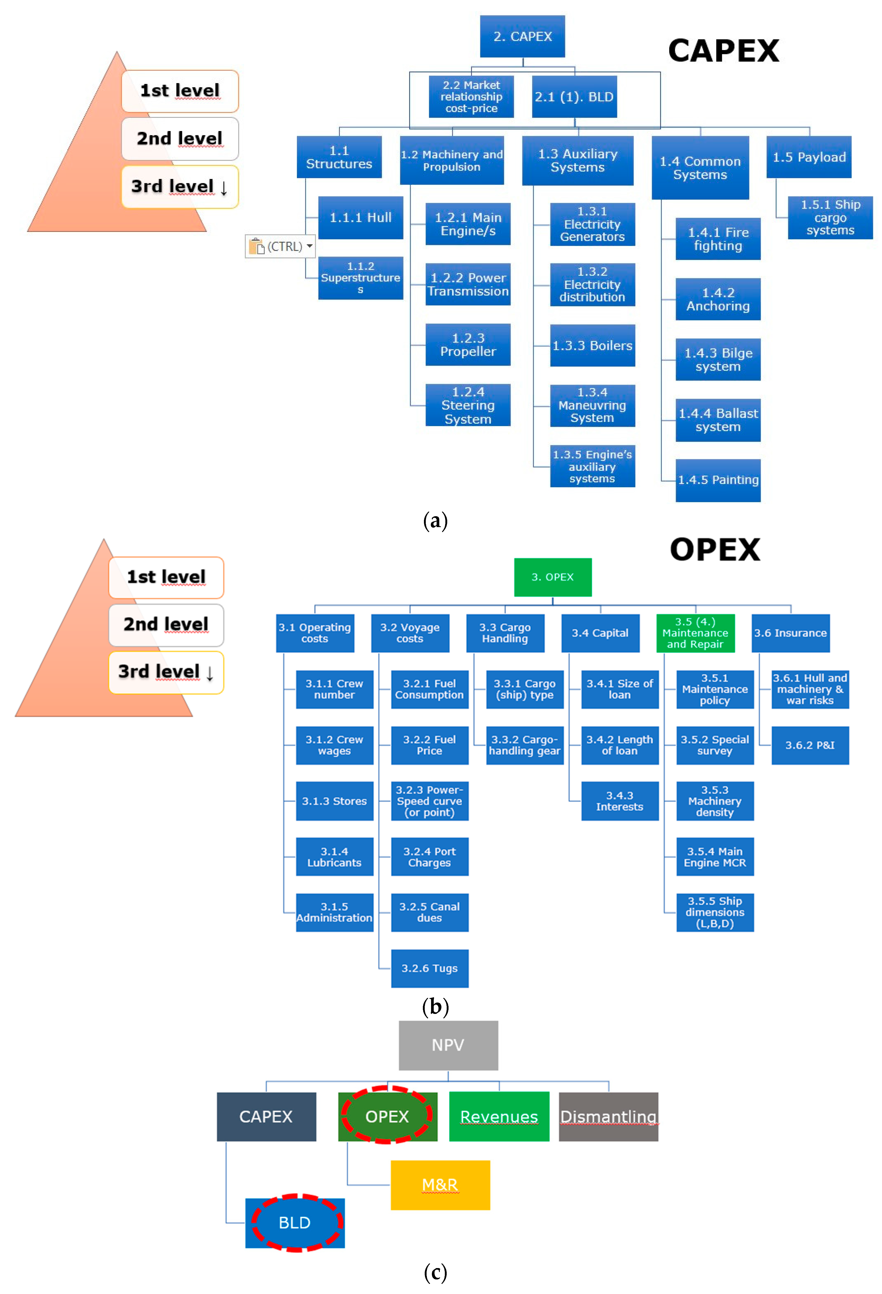
It is worthwhile mentioning that different approaches are possible to combine economic and environmental aspects, for example, converting all incomparable values into monetary values [12]. To better understand the LCPA software and its further improvements developed in this paper, a synthesis of the main topics are proposed in the following sections. As already mentioned, Key Performance Indicators (KPIs) are the base of the LCPA tool. They are performance indicators resulting after the definition of the problem and its cost drivers. There are, respectively, economics and environmental KPIs that play a fundamental role in the decision-making process:

• Building Cost (BLD): It is the costs sustained by the shipyard to build the vessel. Different estimation techniques can be adopted to evaluate this figure, based on the level of details already known in the actual ship design phase. [13].
• Capital Expenditure (CAPEX): It is the funds that a shipowner use to purchase a vessel from a shipyard. This cost is influenced by the type of ship and the installed technological level. It is directly related to the shipyard Building Cost, but it is also influenced by the market situation at a specific moment.
• Operating Expenditure (OPEX): It is the costs related to the vessel normal operation activities [14]. The OPEX changes during the lifetime of the ship, so it is important to determine how much it changes every year (on average), without considering the change of money value due to the discount rate. OPEX takes into account the operating costs, the voyage costs, the costs related to the payload, insurance, interest, and maintenance, and repair costs.
• Maintenance and Repair costs (MandR costs): They are a part of OPEXs, but they can also be used independently to assess costs related to maintenance of systems and structures. This value is directly influenced by the type of systems and maintenance approach adopted.
• Net Present Value (NPV): It is probably the most popular economic measure. It is an index on the profitability, which is evaluated by subtracting the present values of cash outflows (including initial cost) from the present values of cash inflows over time [15].
• Energy Efficiency Design Index (EEDI): It is a parameter introduced by the Marine Environment Protection Committee (MEPC) of IMO in 2011 and it indicates the energy efficiency of a ship in terms of generated CO2 (grams or tons per mile cargo carried). It is calculated for a specific reference ship operational condition. The aim is to drive ship technologies development to more energy-efficient ones [16].
• NOx and SOx emissions (during operation): These parameters measure the grams of NOx or SOx generated per unit of transport work. The regulatory framework is imposing, in recent years, stricter and stricter criteria depending on the sea area where the ship is sailing. NOx emissions mainly depend on the type of engines installed on board, while SOx emissions are mainly related to the type of fuel used to produce energy [17].

Further considerations about the significance of such KPIs can be found in [18]. explicit equations for estimation of all these values, are given in [7,10].

The relations between these KPIs are provided in Figure 1a–c. It is important to denote that the CAPEX value has been described in the paper for the sake of completeness, but during this work, we have always referred to the BLD value.

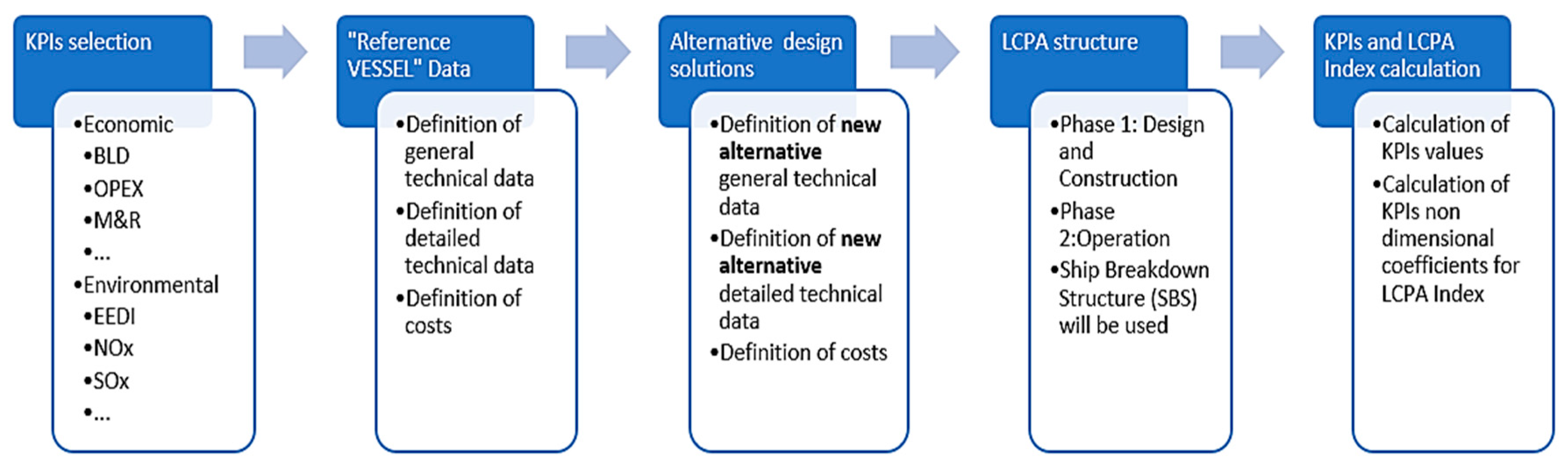
A thorough explanation of the LCPA process is given in [7,10]. Nevertheless, in Figure 2, a block diagram of LCPA steps is provided. The same steps have been followed in the organization of the application case below.

In this work, the M&R costs evaluation have been improved to permit a better evaluation of the OPEX costs: the empiric formulation used in the current first version of LCPA tool could be replaced with a flexible prediction model based on real maintenance actions. The maintenance model, discussed in paragraph 4, would be implemented as part of the LCPA tool. A different energy system layout might also affect BLD value. In this work, such an issue was taken into account.

3. Maintenance Strategies

Maintenance actions ensure that a system performs in the best way during its whole life cycle, preserving its integrity and performances over time. Different maintenance techniques were developed in the last decades to better preserve system capabilities during its life cycle, minimizing the failure rate and downtime. All these actions can be summarized as follows [19].

Corrective maintenance: the simple one without any scheduled action. The operator attends when a failure occurs in switching off the system and performing the maintenance with more or less important economic implications. This approach is based on the belief that the costs sustained for downtime and repairs, in case of a fault, are lower than the investment required for a maintenance program. This strategy may be cost-effective until catastrophic faults occur.

Scheduled preventive maintenance: a step forward in maintenance policy. The manufacturer provides a so-called Mean Time Between Maintenance (MTBM) that is the best working time range when a maintenance action has to be performed to prevent system failure or degradation. In this way, an operator can plan the maintenance services to minimize the impact on working hours and so on costs and profits. The maintenance cycles are planned according to the need to take the device out of service. The incidence of operating failures is reduced. In a complex system with more sub-systems that work together to complete a task, this method can be a better way to plan the maintenance operations.

Performance-based maintenance: often indicated as Condition Based Maintenance (CBM), it is based on the response analysis of multiple sensors mounted on the system to measure actual working parameters like temperature, pressure, fluid levels, and more. Through prediction models, they are automatically compared with average values and performance indexes. Maintenance is carried out when some indicators give the signaling that the equipment is deteriorating and the failure likelihood is increasing. This strategy, in the long term, allows a drastic reduction in maintenance costs, thereby minimizing the occurrence of serious faults. With these previsions, the operator can plan one or more maintenance action only when it is requested and avoiding the interventions when it is not necessary.

These three actions are the most common, but other two maintenance policies can be further mentioned, namely the adaptive maintenance and the perfective maintenance. The first one is applied when the system needs to evolve and adapt for new needs or working contest to extend the system working life; the second one is performed when there is the chance to improve a system with the installation of innovative technology.

In this work, the scheduled preventive maintenance was assumed to develop the maintenance prediction model where the designer could evaluate the quality of the different configuration in relation to maintenance costs and time. This model would improve the current version implemented in the LCPA tool, based on an empirical formulation of the maintenance costs. Preventive maintenance is defined as a semi-deterministic model; however, it gives an effective way to compare different layouts and operational profiles at an early design stage: it takes into account, in fact, that designers could not have access to a large database, recorded dataset, or detailed information on systems they are investigating. The main information needed to set up a scheduled maintenance approach could be more easily obtained from manufacturer manuals. This is the reason why we used the preventive maintenance technique as a starting point [20,21]. The corrective maintenance and the dry-dock maintenance costs have been disregarded in this paper, and they are going to be taken into consideration later in the research activity.

4. Approach Description for Maintenance Costs Evaluation

As just described in the previous paragraph, the model for maintenance costs will be based on the scheduled preventive maintenance and the MTBM (Mean Time Between Maintenance) value [22]. Settled the ship type, the first step is to identify some different design configurations that satisfy the main owner requests, like speed, range, operational profiles, maneuverability performance, environment, and efficiency performance.

• The systems complexity and the huge number of sub-systems and single items installed in each assessed layout impose to choose a solid and structured procedure to evaluate the maintenance actions and related costs over the life cycle. From the builder point of view, the best practice would be to use the so-called Work Breakdown Structure (WBS), defined as a hierarchical and incremental decomposition of a project/system into smaller components: throughout a tree structure at each following iteration, a higher detail level is achieved, breaking up a complex system into a less complex one, and so on [23]. The operator decides when to stop dividing. This top-down structure allows to identify the elements by a single code number and to decide the ones useful in the analysis for the decided level of detail.
• For each selected system or subsystem, the maintenance tasks to include or exclude from the analysis are selected. The higher is the detail level to be considered, the more maintenance tasks have to be included in the tool.
• An MTBM value is needed for every single item selected for the analysis, expressed in working hours or years. The value is usually contained in the system manufacturer manuals with the corresponding maintenance task to be undertaken. The MTBM of an asset is the average length of operating time between one maintenance action and another, and it is usually based on a conservative stochastic distribution (Weibull distribution). Despite MTBM could be supposed a conservative value, if a system or item works out of its optimal working point (for a not negligible time), it is reasonable to suppose that the MTBM value might decrease.
• When defining alternative configurations, it is important to define the system working point. For example, considering a diesel propulsion engine, it is necessary to define its actual working condition expressed in term of MCR percentage and actual working hours. Starting from this information, the off-design working condition can be estimated together with is effects on the MTBM value delivered by the manufacturer. Combining off-design functioning hours and the corresponding power percentage enables to create a dimensionless corrective coefficient to update the actual maintenance plan and its impact on maintenance costs. This concept can be expressed through the proposed Formula (4) obtained through a try and error process based on the real data provided for the project:

  $${\mathrm{MTBM}}^{\prime }=\mathrm{MTBM}-\frac{1}{{\mathrm{h}}_{\mathrm{T}}}\cdot \left[{\displaystyle \sum }_i{\mathrm{h}}_{{\mathrm{ACT}}_i}\cdot \frac{\left({\mathrm{P}}_{{\mathrm{T}}_i}-{\mathrm{P}}_{{\mathrm{ACT}}_i}\right)}{{\mathrm{P}}_{{\mathrm{T}}_i}}\right]\cdot \mathrm{MTBM}$$

  (4)

  where MTBM’ is the new corrected MTBM, the actual value; MTBM is the original manufacturer value; h_ACT is the number of actual off-design working hours; h_T is the number of total actual working hours in one year; P_T is the power corresponding to the optimal working point; P_ACT is the actual power; i is the operational scenario considered, like navigation at 13 kn or navigation at 8 kn, etc. This type of formulation can be applied to the diesel engines for the generation of propulsion.
  If P_ACT and P_T are equal, the engine works at its best and MTBM = MTBM’. The same result is obtained if h_ACT = 0, i.e., the engine is in its best working point. We have assumed that the formulation has an application domain from 20% to 50% of MCR engines power: if an engine works above the 50% of its MCR, the corrective formula is not applied; at the same time for MCR less of 20%, the formula is not recommended.
• The next step requires to consider for each maintenance task the number of man-hours needed, the number of qualified technicians involved, and relevant costs (in €/h). All these values will be combined to calculate a total cost amount for every single task under analysis. If it is required, spare parts will be also included in the cost assessment for each task assumed in the tool.
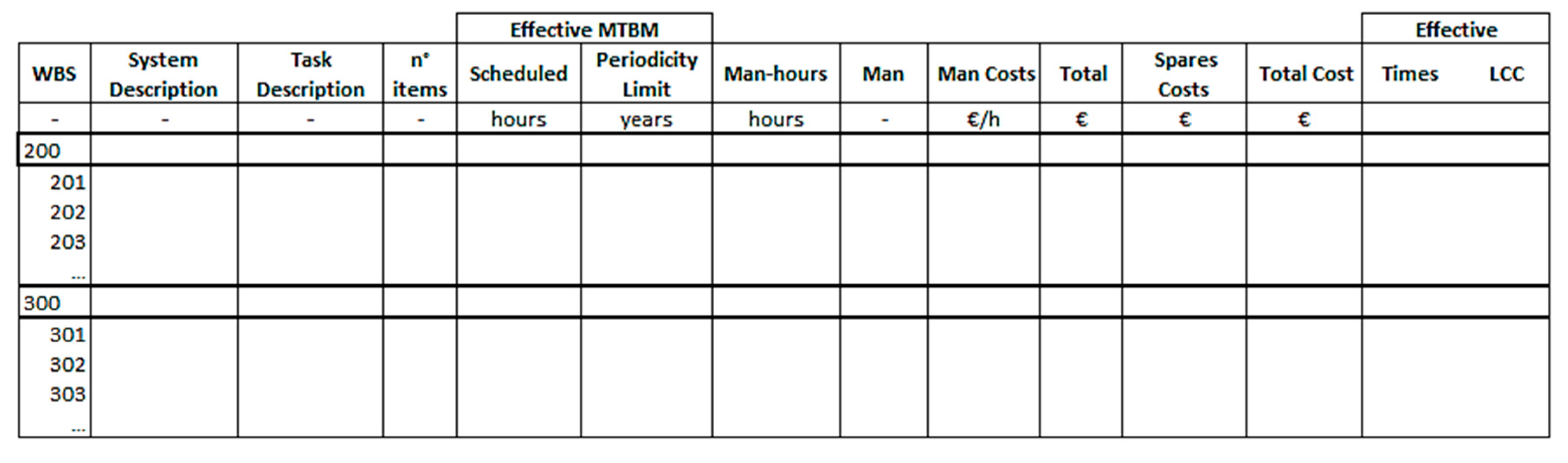
• Once the main system’s actual working hours and the ship life duration (in years) are inserted, the tool automatically calculates the number of maintenance action (times) during the whole life cycle (for each task) and the LCC for the maintenance activity defined as total costs per times. The costs refer to the real ship working conditions through MTBM’, and not to the ideal condition based on the manufacturer’s MTBM. The MTBM or MTBM’ value is used to calculate how many times a particular maintenance action has to be performed during the ship life cycle. The “times” column in Figure 3 is obtained as (effective MTBM)/(item’s total working hours in one year); the LCC for the maintenance activity is calculated as “times” column per “total costs” column in Figure 3.

The tool provides all the information needed to have a general overview of maintenance-related costs over the ship life cycle, with graphical and tabular results. Figure 2 summarizes the maintenance framework where WBS systems and subsystems are written in lines, and the higher is the level of detail, more lines are required.

The columns report (from left to right) a system or subsystem description; the maintenance task description (there could be more tasks for the same WBS voice); the number of same items; the effective MTBM, expressed in working hours or years and corrected with the previous formula; the number of hours dedicated to the task; the number of men required to do the particular task; the man costs; the spares cost (if a spare part is required); the total maintenance task costs; the times that the task is repeated during ship life cycle; the LCC value.

The prediction model is structured to have the WBS, maintenance tasks, number of items, MTBM, man-hours, number of man, and man costs as input data. The model automatically calculates the MTBM’, the total cost of each maintenance tasks, the times each action has to be performed during the ship life, and the costs (indicated as LCC on the right in Figure 3).

During the early design stage, the definition of the ship operational profile is very relevant and has a strong influence on the propulsion system typology. In turn, the propulsion system strongly affects the ships final building cost and the costs linked to operational activity during the whole ship life [16]. From that described above, the LCPA tool has been further enhanced to evaluate the best configuration among some proposed alternative propulsion layouts. Due to the great number of systems and sub-systems installed, the complex connections between them, and the massive amount of required information, it is necessary to further reduce the domain of investigation in this development phase. This work aimed to develop a tool to predict the maintenance costs during the design stage, also when the information available is not so detailed. The intention was to develop a solid and adaptable starting point that could be improved during further interactions or directly customized from the designers themselves over their needs. Once the results of the costs derived from the maintenance tool are inserted in the main LCPA tool, the designer can provide a first attempt to quantify the total ship costs, not only related to building costs but also related to the operating costs. This type of assessment could permit to offer a better and complete overview of the product in a constructive discussion with the customer.

This methodology has been applied to a reference vessel, described in Section 5, to improve its propulsion system. The alternatives systems have been described one by one in Section 6 and are directly compared in Section 7 to identify the best solution.

5. Application Case: Reference Vessel Description

The methodology described in paragraph 4 is now applied on a reference vessel to evaluate propulsion system alternatives. The application platform is a research vessel designed and equipped to navigate the far reaches of the globe. These types of vessels support researches on the sea analyzing temperature gradients, sea chemical composition, carrying out biological or geophysics investigations, or bottom topography. The overall characteristics of a research vessel are identified by the scientific equipment, the specialized personnel on board, the required speed and range. The propulsion system has to be designed to ensure flexibility and a wide range of activities at different speeds. The original propulsion system of a model vessel and proposals of alternative configurations described in the following paragraph would be our starting points for investigations and analysis.

The main vessel dimensions and features are described in

Table 1. Main ship dimensions and performances.

Characteristic	Value	Units
Length over all	94	M
Length between perpendiculars	80	M
Beam	16.6	M
Depth	8.5	m
Displacement	3600	t
Draft	4.64	m
Cruise speed	13	Kn
Max speed	17	Kn
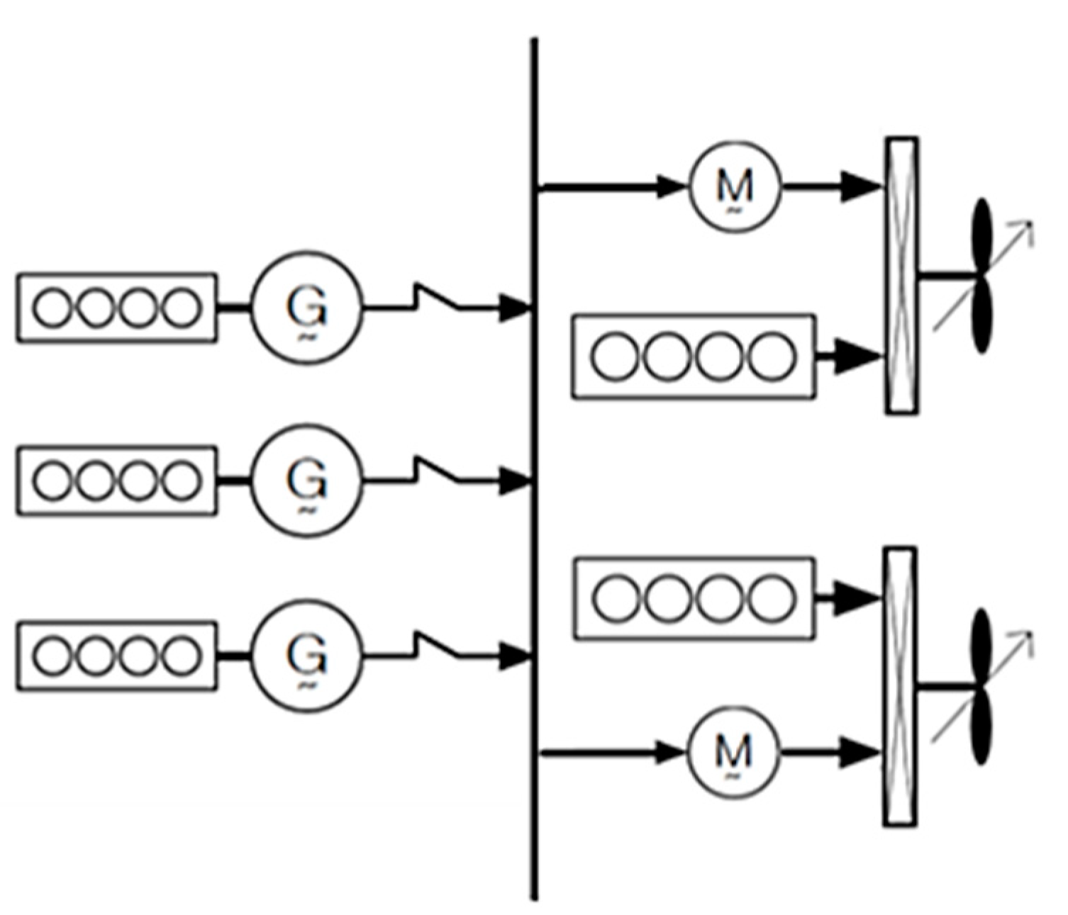
Range	3000	Nm

. The ship is equipped, in the original version, with two independent shaft lines, each provided with the main diesel engine, a small electric motor, a gearbox, and a controllable pitch propeller. Mechanical and electrical systems work together in the propulsion train, optimizing the ship propulsion efficiency and providing the right amount of power delivery to a propeller in any scenario.

This hybrid propulsion system works as a CODELOD (COmbined Diesel and ELectric Or Diesel) where the only electric motors are used for low speeds (up 8 kts), and the diesel engines are instead used for high speeds (from 9 to 17 kts). The electric power generation at 400 V and 50 Hz, in all operating conditions, is ensured by three independent diesel generators connected to the main distribution grid. The emergency power generation is carried out by a dedicated diesel generator, located in a different small engine room. A simple functional scheme of the propulsion and electrical generation layout is shown in Figure 4.

The two propulsion engines are typical four strokes engines based on a supercharged diesel cycle with direct fuel injection. The supercharge is ensured by a turbo-compressor group driven by engine exhaust gases. The two diesel engines installed onboard can supply power output of 2289 kW, irreversible rotation, and opposite turns. A pneumatic system with compressed air is provided for the engines start, while the cooling system is made by a closed high-temperature freshwater circuit and a low temperature opened one.

The electric generation onboard is ensured by three gen-sets located in the main engine room. The electric power produced onboard is mainly used for the “payload” services (that include accommodation services but also scientific equipment power demand) and for the electric propulsion at low speed as well. The gen-sets can produce 650 kWe each at 1500 rpm with an electric output at 400 V and 60 Hz. A single gen-set is made up by a four strokes diesel engine with a direct fuel injection connected to an electric alternator.

Table 2. Main Diesel.

Characteristic	Propulsion Diesel	Diesel Gen-Sets	Units
Number of cylinders	12 V type 45°	8 V type 90°	-
Maximum continuous rating	2289	650	kW
Rotation speed	1050	1500	g/min
Dimension	4100 × 1700 × 2760	4000 × 2100 × 200	mm
Weight	19000	10800	kg
Fuel supply	MDO/MGO	MDO	-

provides a direct comparison between the propulsion types of diesel and the diesel gen-sets (MDO is the acronym of Marine Diesel Oil; MGO stands for Marine Gas Oil).

To increase energy efficiency in a range of low speed, the vessel is propelled by two electric synchronous type motor, one for each propulsion line. They can supply the maximum power output of 250 kW at 1500 rpm and an electric output at 400 V and 50 Hz. Main features are in

Table 3. Electric motor.

Characteristic	Value	Units
Maximum power	250	kWe
Rotation speed	1500	g/min
Voltage output	400	V
Frequency output	50	Hz
Dimension	1160 × 670 × 860	mm
Weight	1030	kg

.

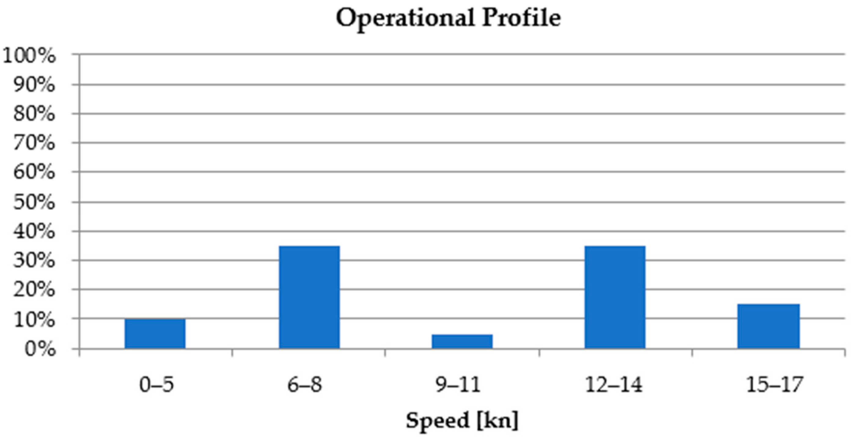
It is important to define one or more profiles before starting the comparative analysis because they can strongly influence the results. As a research vessel, the ship will be optimized to work at two different speed range: low speeds during the maneuvering and oceanographic operations (typically from 0 to 8 knots) and high speeds during shift operation at design or maximum speed (from 12 to 17 knots).

Figure 5 shows the operational profiles of the reference ship: the percentages refer to 165 days/year when the ship is operating at sea. In the remaining 150 days/year, the ship is considered in harbor, and in the remaining 50 days/year, in dry dock. In this scenario, 10% of working life (16 days) is spent at 0–5 kn; 35% (58 days) is spent at 6–8 kn in research operations; 5% (8 days in total) at 9–11 kn during speed transient phases; 35% (58 days) at 12–14 kn at design speed; 15% (25 days) at maximum speed.

All future considerations in this work would be based on this particular operating scenario.

To compare different design alternatives, the first step is to define how the vessel propulsion system works at a different speed and then to identify possible design alternatives to satisfy the operational profile most efficiently. These alternatives will be identified, during this first working phase, as composed by the elements listed below:

• Main Diesel Propulsion Engines (WBS 233)
• Electric Motors (WBS 235)
• Gearboxes (WBS 241)
• Shaft Lines and Bearings (WBS 243 and 244)
• Engines Sea-Water Cooling System (WBS 256)
• Fuel Supply System (WBS 261)
• Diesel Gen-Sets (WBS 311)
• Emergency Diesel Gen-Set (WBS 312)
• Heating, Ventilations and Air Conditioning HVAC System (WBS 514)
• Compressed Air System (WBS 551)

The flexibility of the tool structure ensures a further implementation of new WBS systems.

The operational profile has been related to a ship resistance prediction, to connect each speed to a propulsion power demand, and an electric balance, to better understand the total power demand during ship operations. The propulsion resistance prediction has been coupled to a controllable pitch propeller and the two propulsion diesel engines described above. A general overview of the ship propulsion system and ship power demand has been provided and used as a starting point.

Electric Load Balance

The term propulsion system (as we considered it in this work) is not only referred to the power required to move the ship, produced by two main diesel engines and two small electric motors, but it takes into account the electric production as well. This electrical power is needed not only for the electric propulsion motors, but also for the bow or stern thrusters, auxiliary propulsion systems, hotel loads, and the scientific equipment. In the original vessel configuration, this power demand is ensured by three diesel gen-sets (please refer to Figure 4 and Table 1) that satisfy the total electrical power demand in all ship operative conditions. The electric load balance of the reference vessel is available in Table 4. Utilization factors in Table 4 appear to be far from ideal figures, and, in particular, 95% and 88% relevant to summer harbor and winter harbor conditions are not in principle practicable, even though such values refer to a ship currently in operation. This configuration is, therefore, suitable for further improvement.

Harbor, Maneuver, and Navigation are the three phases considered in the electric balance. Each operational phase is split up in summer and winter condition to have an overview of power demand during different seasons.

For each column in

Table 5. Working hours in a year for each WBS analyzed (see Abbreviation List at the end of the paper). Reference configuration.

Operation	Speed	n D/G	% D/G	WBS 233	WBS 235	WBS 241	WBS 243	WBS 256	WBS 261	WBS 311	WBS 514	WBS 551
	kn	-	-	hours	hours	hours	hours	hours	hours	hours	hours	hours
Port	0	1	0.95	0	0	0	0	0	1800	1260	2880	900
Manoeuvre	1 to 5	3	0.71	0	307.2	384	384	192	192	268.8	307.2	96
Research	6 to 8	3	0.70	0	1392	1392	1392	1113.6	696	1392	1113.6	348
Transient	9 to 11	2	0.58	96	0	192	192	153.6	192	134.4	153.6	48
Navigation	12 to 14	2	0.58	1392	0	1392	1392	1392	1392	974.4	1113.6	348
Navigation	15 to 17	2	0.58	600	0	600	600	600	600	420	480	150
				2088	1699.2	3960	3960	3451.2	4872	4449.6	6048	1890

, an indication of several gen-sets, in use, and their utilization factor has been provided. All this information gives an overview of how the propulsion configuration works in different scenarios during its working life. Besides, Table 5 shows for each scenario the number of working hours in a year of each WBS considered and described in paragraph 5.

Table 4 and Table 5 refer to reference propulsion layout, and the information would be used as a solid base for the further considerations discussed in paragraph 6. All this conclude the preliminary phase.

6. Application Case: Design Alternatives

Starting from information identified in paragraph 5, it is possible to evaluate few alternative propulsion layouts to achieve a more efficient system, with possible advantages on building costs and operative costs, including all maintenance actions. In the following lines, three alternatives configurations are proposed: they have been designed focusing on a reduction in WBS working hours and/or maintenance costs.

6.1. First Design Alternative—Power Take-Off

The first alternative layout (identified as S1) proposes the introduction of a Power Take-Off (PTO) in the original propulsion system. In particular, the PTO is supplied by the main propulsion Diesel with the double aim to reduce the working hours of one or more diesel gen-sets, and to achieve a better working point both for diesel engines and for the gen-sets (compared to the original layout). Engines power size are the same as reference vessel, and the PTO is active only from 9 kn to 17 kn; up to 8 kn, the configuration works exactly as the original one. So, for the harbor, maneuvering, and navigation activities up to 8 kn, the power demand is supplied by two electric motors (for propulsion and maneuvering) and by the diesel gen-sets, as reported in

Table 6. First alternative configuration power-use analysis results. Focus on changed WBS working hours.

Speed	PB	PTO	n D/G	% D/G	WBS 235	WBS 311
kn	kW	kW	-	-	hours	hours
0	0	0	1	0.95	0	1260
1 to 5	83	0	3	0.71	307.2	268.8
6 to 8	320	0	3	0.70	1392	1392
9 to 11	807	500	1	0.41	192	67.2
12 to 14	1760	500	1	0.41	1392	487.2
15 to 17	3617	500	1	0.41	480	240
					3763.2	3715.2

. After 8 kn, the propulsion starts to be supported by the diesel engines, so, after this point, it is possible to use the electric motors (used as PTO) instead of the diesel gen-sets to supply the power needed for hotel services. Figure 6 clarifies this working operation.

Table 6 reports the configuration analysis in terms of propulsion power (P_B), PTO, number of active gen-sets and their working point (%), and WBS voices that have changed their working hours. The analysis put in evidence the PTO power impact during navigation phase: after 8 kn, the PTO supplies more electrical power in the network, so it is possible to use only one gen-set, compared to two in the original configuration. There in an increase in for WBS 235 working hours, while a decrease is evident for WBS 311 working hours.

It is important to underline that the gen-set in use works at 41.5% of its nominal power, and for diesel gen-sets, it is not a good solution in terms of fuel consumption and maintenance. This consideration took us to consider a second alternative configuration to solve this problem.

6.2. Second Design Alternative—Power Take-Off with Higher Power Size

The second alternative (S2) layout proposes the introduction of a higher power size PTO and also a higher power size for gen-sets to obtain an efficient working point. This solution could be identified as an evolution of the previous one, with the main aim to reduce to zero the number of gen-sets used during the navigation phase. So, the configuration layout is the same, as defined in 6.1, and differs only for the items size and working point. Figure 6 continues to represent the system layout. The new proposal increases the electric motors size (also used as PTO) from 250 kW to 390 kW and gen-sets size from 650 kW to 850 kW. This option permits to satisfy the total amount of power demand in the navigation phase using the PTO only. The total number of simultaneous active gen-sets, in the worse scenario, decreases from three to two, but from a reliability and redundancy perspective, the third gen-sets are used as a stand-by element. The results achieved in this way have been represented in

Table 7. Second alternative configuration power-use analysis results. Focus on changed WBS working hours.

Speed	PB	PTO	n D/G	% D/G	WBS 235	WBS 311
kn	kW	kW	-	-	hours	hours
0	0	0	1	0.850	0	1260
1 to 5	83	0	2	0.850	307.2	268.8
6 to 8	320	0	2	0.810	1392	974.4
9 to 11	807	780	0	-	192	0
12 to 14	1760	780	0	-	1392	0
15 to 17	3617	780	0	0.600	480	120
					3763.2	2623.2

. It puts in evidence how the PTO supplies the total electric power demand during the navigation phase over 8 kn. The two diesel engines are the only active power generators during the navigation from 9 to 16 kn, both in summer and winter.

Comparing Table 7 to Table 5 (S0 configuration), the higher power sizes ensured a better gen-sets working point in all conditions, less working hours, a reduction in fuel consumption, and stress on the mechanical elements. A reduction of working items was ensured: from three to two in maneuver; from two to 0 during navigation. The gen-sets total working hours were also reduced (from 4449 to 2623), but the working hours of electric motors were increased from 1699 to 3763. Main diesel working hours were the same, as described in Table 5 and Table 6, but the working point was higher due to the PTO supply during navigation from 8 kn to 17 kn.

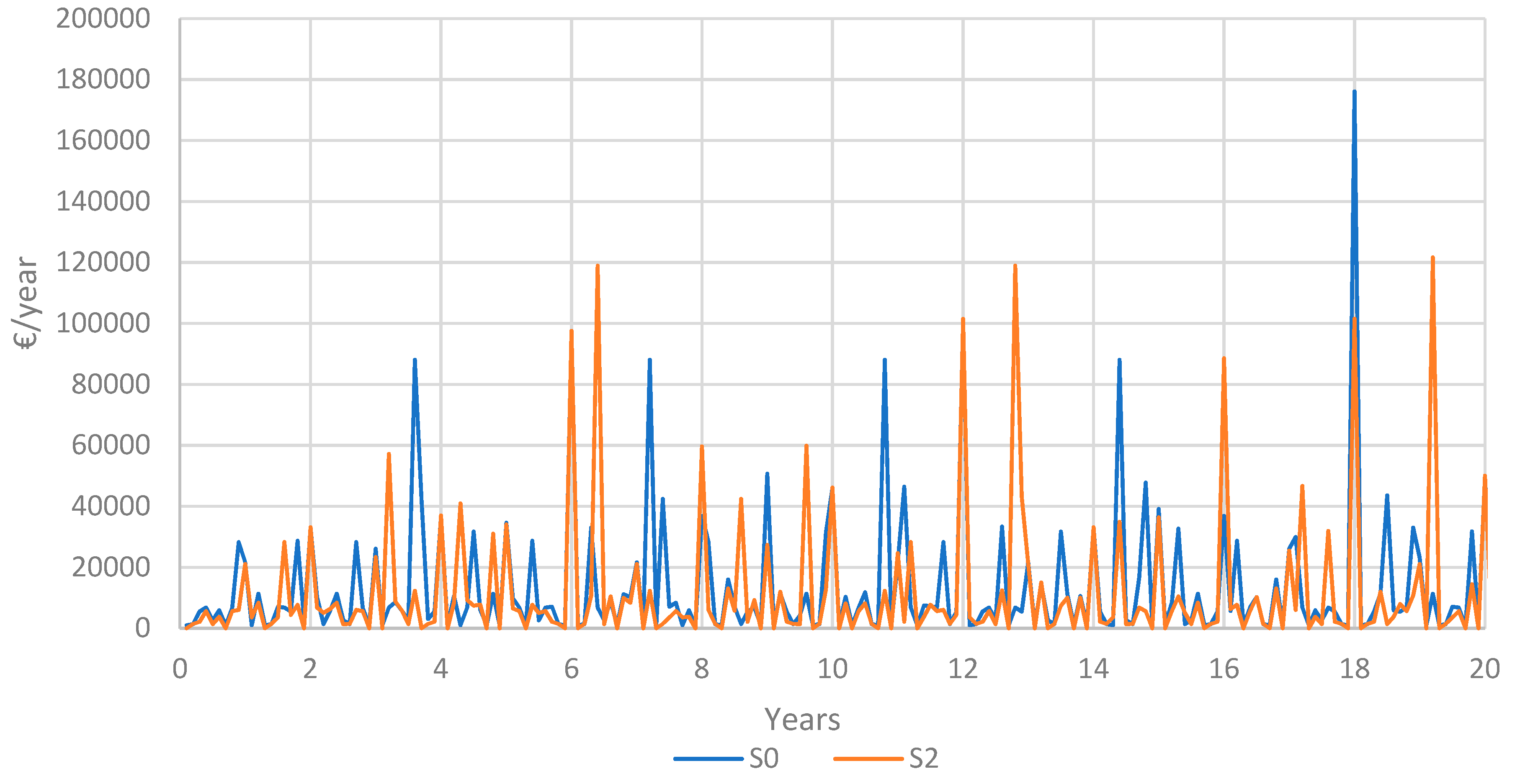
The remaining systems have the same working hours as S0, but the active units are lesser with a positive influence on maintenance tasks. All this information are the input data to the maintenance tool described in paragraph 4. The comparison in terms of a maintenance plan, between reference layout S0 and layout S2, is shown in Figure 7. The blue line is referred to reference layout (S0), while the red one to second alternative layout (S2): over 20 years, the S2 maintenance actions are, on average, less expensive than the original layout. The MTBM correction affects not only the distribution of the costs over the years but also the maintenance periodicity, that is out of phase than the original maintenance plan. From the owner point of view, this type of results presentation provides an overview of M&R, permitting to schedule when could be better to sell the ship to prevent excessive M&R costs.

Paragraph 7 provides a costs comparison between all alternative solutions described here.

6.3. Third Design Alternative—Total Electric

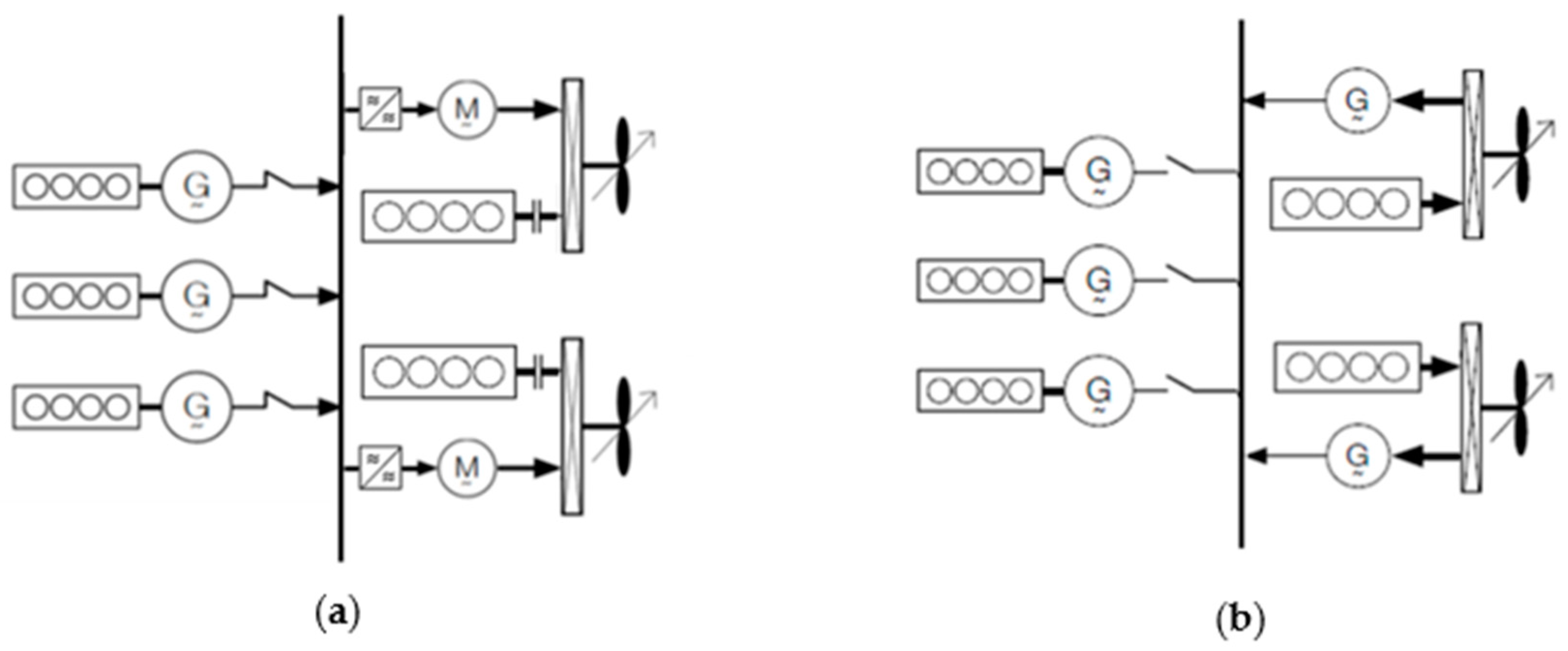
The third alternative layout (S3) proposes a complete change in the propulsion layouts through the introduction of fully electric propulsion. Instead of the two main Diesel engines, two main electric motors have been installed, supplied by four diesel gen-sets. This configuration could be an optimal choice for ships that have a special environment request, as a research vessel, and need a large amount of electric power available during the operational phases. A comparison between hybrid propulsion and fully electric propulsion, on maintenance perspective, could be interesting. As synthesized in Figure 8, usually this configuration is composed of diesel gen-sets; main switchboards; propulsion transformers and frequency converters; electric engines for propulsion; gearboxes (optional) and propellers.

This configuration ensures high power flexibility, and so it is not necessary to divide the speed range as done before. From 1 to 17 kn, the total electrical power demand will be satisfied by a variable number of gen-sets, regulated by onboard automation. The electrical motors are only used as main propulsion engines: a PTO is not considered in this configuration.

The two electric propulsion engines have a power size of 1800 kW each, to ensure a 17 kn maximum speed. The gen-sets have to satisfy the power requested at 17 speed (by propulsion) and the power requested by the hotel loads during navigation, equal to 760 kW in summer navigation (worse condition). So, the gen-sets are four units of 1150 kW each. This layout ensures the redundancy of power generation units and, at the same time, permits a high control over the electrical power generation during the different operational phases.

Table 8. Third alternative configuration power-use analysis results. Focus on changed WBS working hours.

Speed	PB	PTO	n D/G	% D/G	WBS 233	WBS 235	WBS 311
kn	kW	kW	-	-	hours	hours	hours
0	0	0	1	0.550	0	0	900
1 to 5	83	0	2	0.650	0	384	192
6 to 8	320	0	2	0.870	0	1392	417.6
9 to 11	807	0	2	0.700	0	192	96
12 to 14	1760	0	3	0.680	0	1392	1044
15 to 17	3617	0	4	0.960	0	600	600
					0	3960	3249.6

proposes an overview of WBS that changed their working hours.

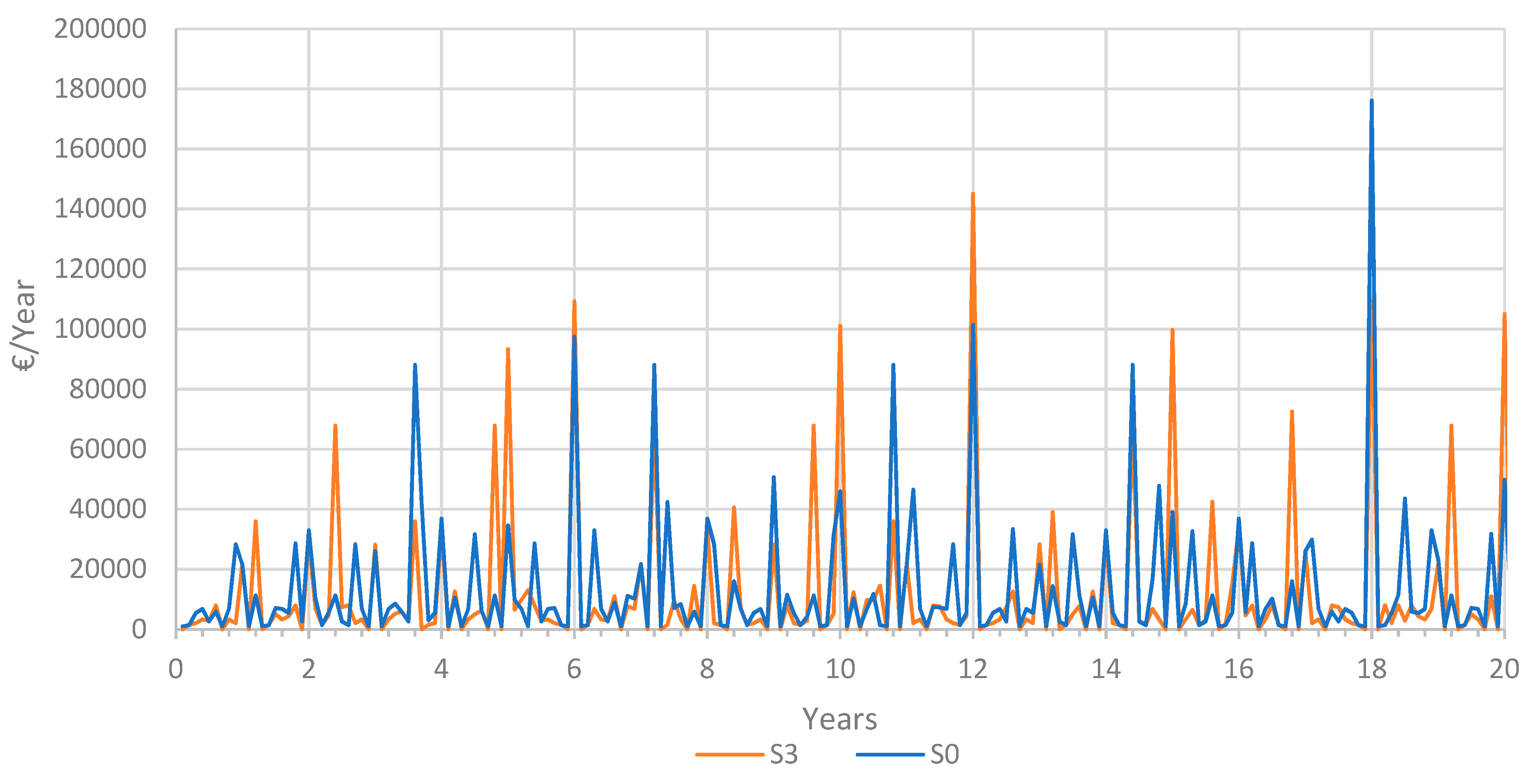
Figure 9 provides an overview of the comparison of a maintenance plan between S0 and S3. M&R costs are, on average, less expensive than the original ones with a better peaks distribution over the years. Plus, a fully electric solution is eco-friendly, that is not a negligible aspect for a research vessel.

The costs comparison is proposed in paragraph 7.

7. Application Case: Results

Four different solutions were analyzed in this paper: the traditional diesel configuration (S0), the PTO solution (S1), the PTO of higher power size, and the fully electric one (S3).

Table 9. Results of the layout comparison.

Data		Reference S0	S1	S2	S3
BLD	[€]	70,038,000	70,697,980	72,715,388	76,714,838
CAPEX	[€]	98,877,176	99,808,913	102,657,018	108,303,301
OPEX	[€/year]	4,026,187	3,937,086	3,820,971	3,980,591
M&R	[€/year]	452,777	476,177	365,856	409,999
NPV	[€]	205,493,593	205,369,584	205,584,835	214,916,381
EEDI	[gCO2/t*kn]	266.63	251.09	260.68	260.68
SOx	[gSOx/t*kn]	4.99	4.70	4.88	4.88
NOx	[gNOx/t*kn]	11.64	10.96	11.38	11.38

provides the results of the total costs obtained with a complete LCPA analysis: we mainly focused on BLD, OPEX, and M&R values to compare the solutions. EEDI, Sox, and NOx are approximated values, but they can give an idea of the solution quality. Speaking in terms of BLD, the reference ship layout (S0) is the less expensive, while the fully electric configuration, as expected, is the most expensive; solution S1 and S2 are very similar, S2 is penalized by the third gen-sets installed for a redundancy aspect but not needed in terms of power generation (two gen-sets covered all scenarios). In terms of OPEX, the best solution is S2, while the reference configuration (S0) is the worse. It is important to remind that OPEX value includes fuel consumption, so, this value could also be read as, S0 has a higher fuel consumption than S2 and S3. For each configuration, fuel consumption has been calculated, combining the utilization factors and the complete engines diagrams. Referring to data reported in Table 5, Table 6, Table 7 and Table 8, the results obtained are truthful.

The M&R are lower in S2 and higher in S1: as expected, S2 is the configuration that has been designed to ensure engines’ better working point and this is underlined in OPEX and M&R values that are the best. S1 that has a worse working point, as shown in Table 8, also has higher M&R costs: a bad engine utilization reduces the MTBM and increases the maintenance times over ship life cycle.

The EEDI value points out that all alternative configurations have better efficiency and lower emissions than the reference one. S1 is the solution with the lower EEDI value, but we should underline that value in S2 is affected by the third gen-set installed as a stand-by unit. The EEDI value is a function of installed power.

It is important to note that despite S1 has worse engines working point, and therefore higher M&R is the best solution. Speaking in terms of NPV, the total value not differs so much from the other ones.

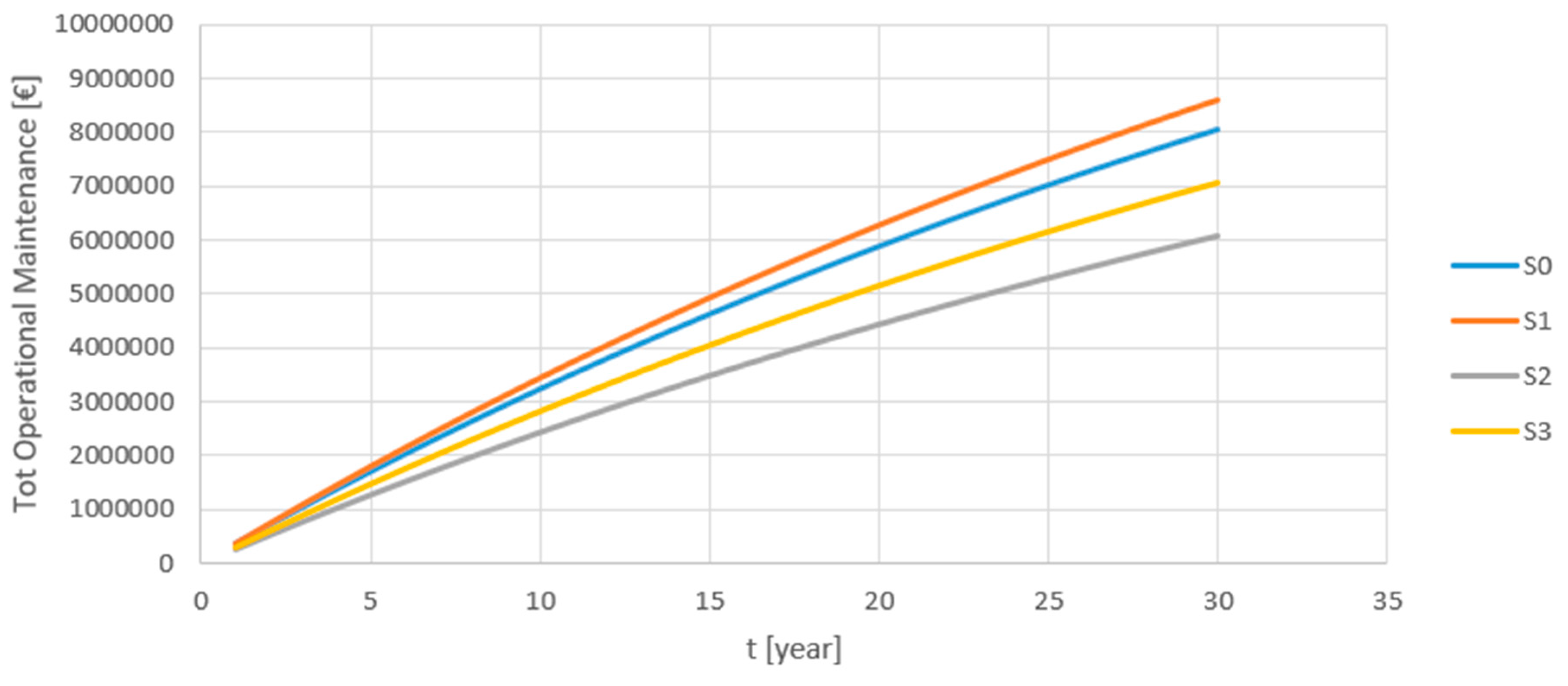
In Figure 10, it has been reported the LCC values maintenance over time for the four layouts S0, S1, S2, S3. As just said, solution S2 is the best in terms of operational maintenance; indeed, it has been designed to minimize maintenance costs. An unexpected result is given by solution S0: it is a cheaper solution than S1 even though the main engines are used less efficiently than in solution S1 (characterized by the introduction of the PTO).

From these results, it is also possible to see that the fully electric, besides being the most expensive solution, will not guarantee a significant advantage during the years. From this analysis, we can also say that, at least for our application case, it is not true that the most expensive solution is always the best in terms of maintenance costs. Analyzing the last years of the ship life in the graph (25–30 years), it seems that solution S2 would bring a good saving compared to the original solution.

Table 10 provides the results in terms of dimensionless index ready for the LCPA calculations: the coefficient is always defined between zero (worst) and one (best). S1 is the best, and S2 is the second-best solution, even if it is affected by the power surplus installed. Not purchasing the third gen-set, decision subjected to owner agreement, implies less BLD and M&R. The S3 is the worst layout, but it is important to stress that LCPA tool does not take into account noise and vibration problems, new possible weights distribution onboard, engine room locations, and off-limits routes.

The last column in Table 10 is part of the LCPA tool structure: for each KPI, a weight has been assigned. The assignation is arbitrary and given by the designer or the owner or the shipbuilder. In this case, we selected BLD and M&R as most interesting KPIs, followed by OPEX. In this perspective, despite NPV value is one of the most popular economic indicators, it has not been deeply discussed and analyzed during this work focused on maintenance actions and costs: the weight assigned in Table 10 is equal to 0 for this reason. The NPV value does not present significant changes in S0, S1, and S2 because the technology used in the propulsion system is the same (i.e., diesel engines), while the S3 configuration employs large electric motors as main propulsion item.

The same results are shown in Figure 11 below.

8. Conclusions

For a research vessel, all the necessary data have been provided to start developing and assess a maintenance prediction model based on a real maintenance plan and not on a parametric formulation. The methodology described in Section 4 is a result of multiple interactions: it has been developed for the reference vessel only and then readapted to a general application for various vessel types. Figure 3 provides a simplified scheme of the maintenance tool and calculation structure.

During the tool development, a corrective Formula (4) for diesel engines MTBM has been defined to take into account design mistakeS on the maintenance costs. Application cases have been carried out on a research vessel, as exposed in Section 5 and Section 6. Different propulsion solutions have been identified, and the tool can characterize them in terms of different performances; but, at the same time, it not so simple to identify the best solution because of the final evaluation that is strictly related to the stakeholder point of view.

Further improvements could derive from the following activity:

• to improve the modeling of corrective maintenance actions and dry dock actions;
• to improve Formula (4) with a major number of real maintenance data and with the implementation of engines overfeed curves.