Validating an Operational Flood Forecast Model Using Citizen Science in Hampton Roads, VA, USA

Abstract

Changes in the eustatic sea level have enhanced the impact of inundation events in the coastal zone, ranging in significance from tropical storm surges to pervasive nuisance flooding events. The increased frequency of these inundation events has stimulated the production of interactive web-map tracking tools to cope with changes in our changing coastal environment. Tidewatch Maps, developed by the Virginia Institute of Marine Science (VIMS), is an effective example of an emerging street-level inundation mapping tool. Leveraging the Semi-implicit Cross-scale Hydro-science Integrated System Model (SCHISM) as the engine, Tidewatch operationally disseminates 36-h inundation forecast maps with a 12-h update frequency. SCHISM’s storm tide forecasts provide surge guidance for the legacy VIMS Tidewatch Charts sensor-based tidal prediction platform, while simultaneously providing an interactive and operationally functional forecast mapping tool with hourly temporal resolution and a 5 m spatial resolution throughout the coastal plain of Virginia, USA. This manuscript delves into the hydrodynamic modeling and geospatial methods used at VIMS to automate the 36-h street-level flood forecasts currently available via Tidewatch Maps, and the paradigm-altering efforts involved in validating the spatial, vertical, and temporal accuracy of the model.

1. Introduction

Inherently, hydrodynamic models are best validated with water level sensors, due to the precision afforded by defining the timing and depth of inundation at a location in an automated manner [1,2,3,4]. As a result of decreased technological costs, low-cost low-energy networks of water level sensors leveraging the Internet of Things (IoT) are beginning to dramatically densify the flood data available in urban environments in coastal areas throughout the world [5,6]. Hampton Roads, VA, USA, hosts one of these IoT networks called StormSense. The network functions as a flooding resiliency partnership between the Virginia Commonwealth Center for Recurrent Flooding Resiliency (CCRFR) and several coastal cities in Hampton Roads [7]. The network’s primary goal is to monitor and transmit automated flooding alerts in real time when inundation occurs [8,9] However, an additional function of these sensors is the integration with federal sensor data from the US National Oceanic and Atmospheric Administration (NOAA) and the US Geological Survey (USGS) to validate and improve the Virginia Institute of Marine Science’s (VIMS) flood forecast models [7,8,9].

However, when it comes to logistical considerations and the high cost of maintenance involved in deploying traditional in situ or remote water level observing systems, these factors can limit sensor density when even finer scale data are needed, and therefore impede these systems’ ability to accurately monitor fine-scale environmental conditions [8,10]. In recent years, the combination of youth who are increasingly globally connected to the internet, and a growing population of retired professionals, poses an opportunity to create a wide-ranging and diverse network of citizen scientists with the capacity to span multiple societal themes [11,12]. Citizen science is public participation in conducting scientific research by non-professional scientists, typically following some form of informal training on data collection. While not a panacea for all inundation monitoring needs, citizen scientists can augment and enhance traditional research and monitoring. Their interest and engagement in flooding resiliency issues can markedly increase spatial and temporal frequency along with an effective duration of sampling. This can reduce time and labor costs, provide hands-on science, technology, engineering, and mathematics (STEM) learning related to real-world issues, and increase their public awareness and support for the scientific process. Naturally, a lack of sufficient professional oversight in citizen science endeavors can introduce caveats to overcome before wide-scale inclusion in an established coastal observing system, yet progress in this underutilized resource is promising [4].

First seeing significant adoption in the US in the aftermath of 2012 Hurricane Sandy, citizen science flood monitoring efforts first became useful through mobile phone pictures capturing inundation with a time-indexing landmark in view, such as a clock tower or local bank clock [13,14]. These pictures gave credence to the digital medium with the advent of enhanced-GPS, which leverages the Global Positioning System’s (GPS) satellite constellation along with nearby cell towers to better triangulate a user’s position on the ground. These tools have now begun to rival the utility of government-sponsored post-event flood monitoring efforts, such as the USGS’ high water marks [15]. While the latter approach affords confidence for model validation through a trusted agency for superior accuracy, the former possesses a greater capacity to document everywhere flooding occurs, with the inherent risk of potentially less accurate validation data. Regardless, collection of data at the local scale in public spaces where flooding is prevalent, such as streets, public right-of-way access spaces, and parks, can improve model prediction by properly resolving flow around small-scale features in the built environment [12]. Additionally, the model’s predictive acumen can be enhanced via improved calibration of assumptions, such as: (1) Better friction parameterization of different land cover types, (2) improved aerial elevation estimates of occluded roadway overpasses, and (3) identification of tidally-susceptible subterranean drainage infrastructure junctions (where tidal waters can enter city streets several blocks from the water’s edge). Thus, quality assurance of flood validation data near these fine-scale features can become valuable model improvement assets through the proper training of a citizen scientist network [16].

Through technological progression, many effective methods for mapping inundation and flood depths have been developed using GPS, photo tagging, Augmented Reality (AR) image landmark recognition, and Quick Response (QR) codes [7,11,13]. Naturally, the emergence and growing necessity of smart phones in modern living has popularized the prominence of these recording methods. Additionally, the ease of access afforded by mobile applications for making insurance claims, verifying flooding for municipal government attention, and greater scientific aspirations has increased the intrinsic value of personal flood mapping [17,18]. Thus, flood-observing mobile applications, like “MyCoast” [19] and “Sea Level Rise” [12], or crowdsourcing web data geo-forms, like those implemented at the state [20,21], country [22,23], and international level [24], have emerged for myriad resiliency purposes. Typically, these applications exist to verify claims of flooding, validate flood forecast models, or inform long-term flood planning efforts [19,20,21,22,23,24]. Mobile flood mapping platforms and applications have recently become information repositories that provide a living data archive of flood observation data with sufficient recording frequency and data density in urban areas where flooding is prevalent [25]. However, these tools have been shown to be of less utility in rural coastal areas, where statistically, less people are present and motivated to vigilantly monitor inundation, and where enhanced-GPS signal strength is diminished due to less reliable cellular broadband coverage [26]. Yet, over time, these data sets can even become their own autonomous data-driven flood prediction models via sea level trend extrapolation when combined with Digital Elevation Models (DEM) [16]. Thus, high-resolution street-scale hydrodynamic models have recently found a new way to validate their predictions, and a cost-effective method for correcting erroneous elevation assumptions from aerial lidar surveys. This includes occluded areas in heavily canopied flood-prone areas and built infrastructure, such as box culverts, highway overpasses, and bridges that impact proper hydrologic drainage in flooding conditions [27].

A proactive and safe way to leverage these technological advances in citizen science flood monitoring methods without waiting for a major storm to elucidate inaccurate model assumptions is to map the incidence of “nuisance flooding.” This approach takes advantage of mapping inundation in places where it frequently occurs with minimal danger to the reporter, and can identify issues with modeled flood forecasts without waiting for a major tropical or extratropical storm event to identify them first [12]. Hampton Roads, VA, USA experiences tidal nuisance flooding 12 to 18 times a year [28]. This is a frequency that amounts to no less than one cumulative week per year that low-lying streets in the region are inundated [29,30]. This chronic flooding fatigue can make it easy to forget that intermittent tidal flooding events cost cities and their residents time and money [30,31]. Of these tidal inundation events, the highest astronomical tide of the year has become known as the king tide [20]. While not a scientific term, a king tide is a name that refers to an exceptionally high tide, without the consideration of atmospheric amplification from wind or waves [21,23]. These predictable king tide events can be estimated far in advance and make coordinating and mobilizing a volunteer effort to track their inundation extent easy, while maximizing the opportunity for local weather impacts to potentially amplify the inundation observed [20].

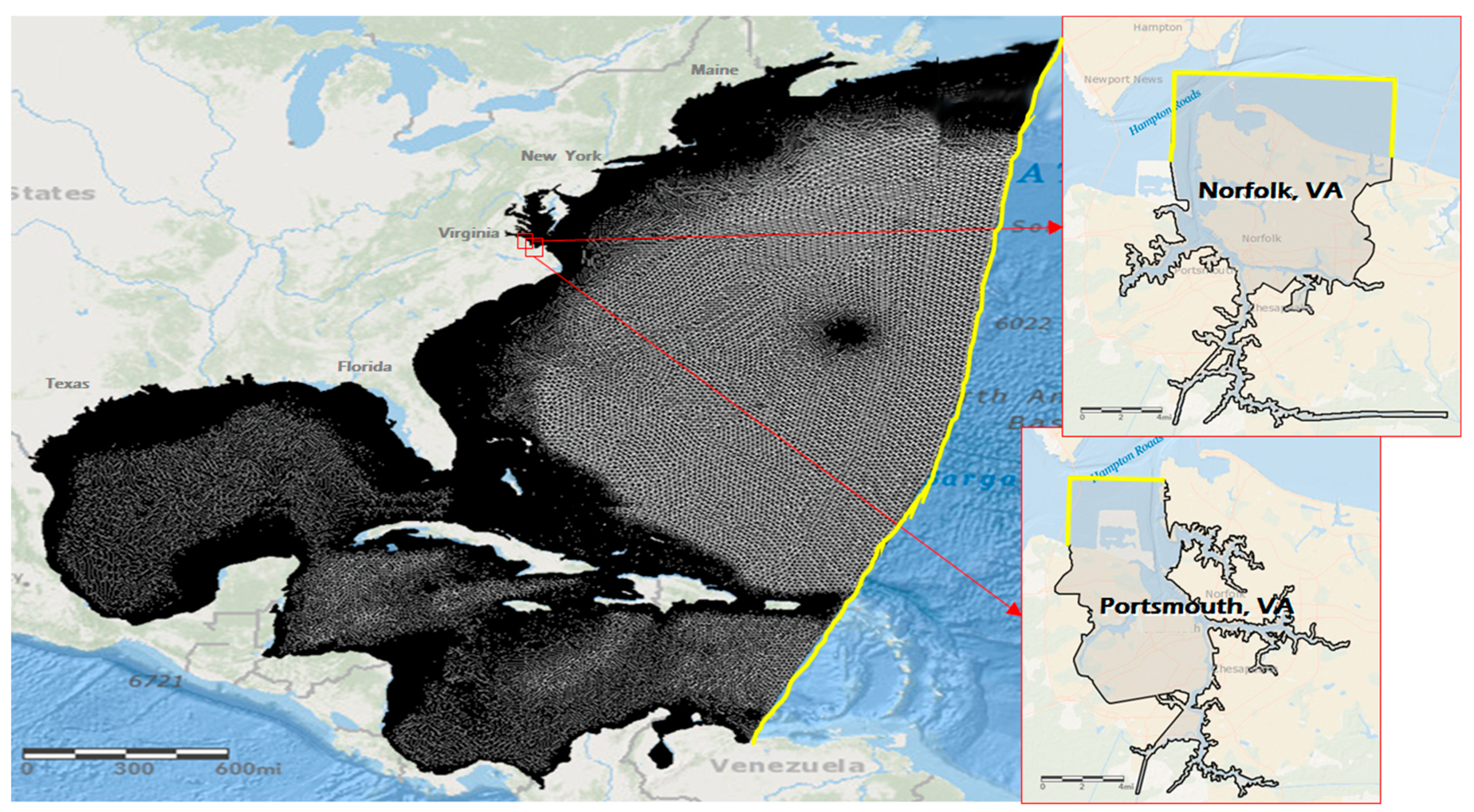
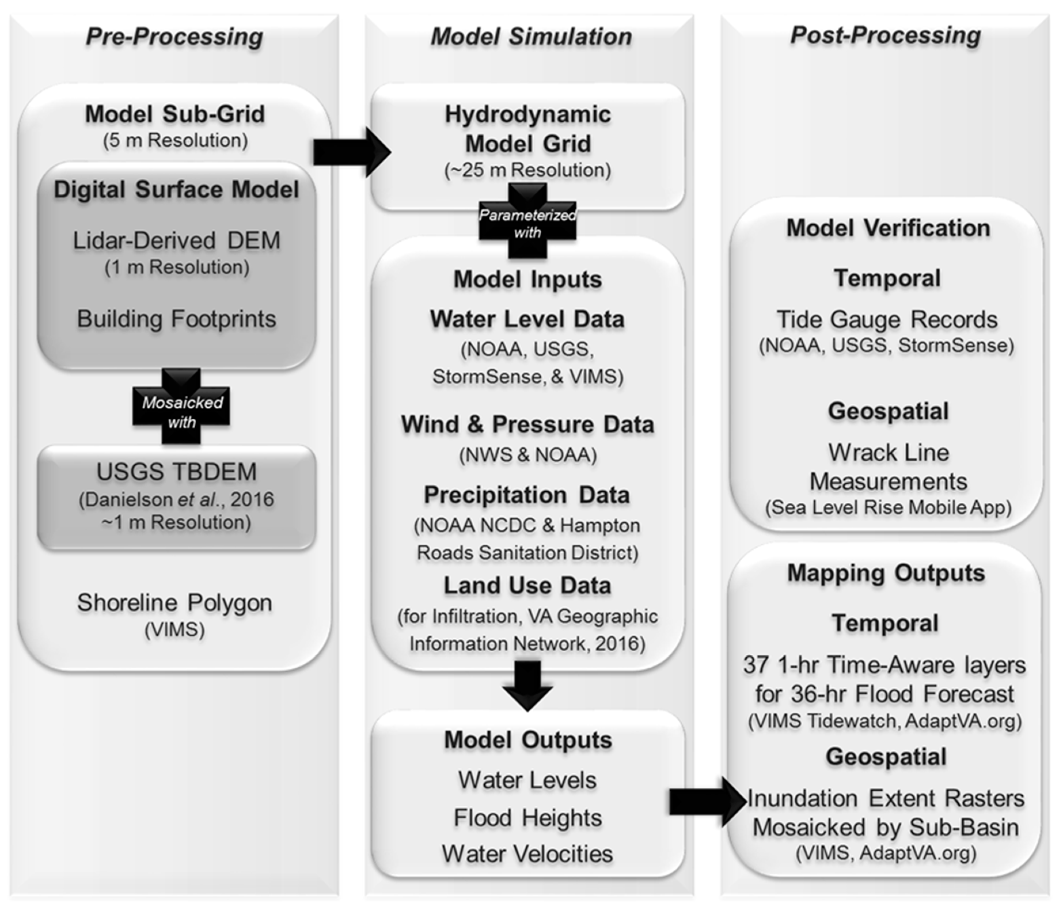
This manuscript describes methods employed at VIMS to disseminate automated inundation forecasts called Tidewatch Maps. The forecasts function as an operational flood forecast model, which leverages the open-source Semi-implicit Cross-scale Hydro-science Integrated System Model (SCHISM) to automatically compute storm tide simulations throughout the entire US East and Gulf Coasts (Figure 1). SCHISM then translates those water level outputs to 220 localized lidar-derived sub-grid modeled sub-basins ranging from 1 to 5 m resolution to calculate 36 1-h geospatial flood depth layers covering all of Tidewater Virginia. SCHISM and the Tidewatch Map currently download inputs and update mapping outputs twice daily, every 12 h. Reliable inundation prediction depends upon accurate simulation of large-scale inundation of the tidal long wave during a king tide to successfully propagate from the ocean, through the continental shelf, estuarine systems, into creeks, and ultimately city streets, and rigorous conservation of fluid momentum and mass as flood waters permeate the built environment. These Tidewatch forecast maps were benchmarked in Hampton Roads by >100,000 GPS-reported high water marks collected by citizen scientists during two king tide flooding events occurring in 2017 and 2018.

The following sections highlight how coastal communities are being meaningfully engaged in coastal ocean observing mechanisms and the research efforts they support. What follows is a description of: (1) A citizen science flood mapping project called Catch the King based in Hampton Roads, VA, (2) effective volunteer training methods using cell phones to provide meaningful GPS observations for effective model validation, (3) hydrodynamic modeling approaches used for expediently simulating and publicly mapping near-term inundation, along with (4) a summary of the results. The paper concludes with an identification of the modeling and monitoring challenges and potential solutions for modeling and citizen science efforts in the future.

2. Methods

2.1. Citizen Science Flood Monitoring Data Collection

Catch the King is a citizen science GPS data collection effort centered in Hampton Roads, VA, which aims to map the king tide’s maximum inundation extents, with the goal of validating and improving predictive models for future forecasting of increasingly pervasive nuisance flooding [16]. The aptly-named effort is the world’s largest simultaneous citizen science GPS flood data collection effort, and it is aimed at benchmarking the highest astronomical tide of the year, the king tide. Certified by Guinness World Records for having ‘the most contributions to an environmental survey’ on the planet, Catch the King was effectively publicized and promoted by the local news media, in Hampton Roads, VA [27,32]. High citizen engagement during a king tide inundation event resulted in an average of 572 GPS-reported high water marks being recorded per minute during the hour surrounding the king tide’s peak [12]. Time-stamped GPS flood extent measurements and photographic evidence were reported via the free ‘Sea Level Rise’ mobile application, coinciding with the king tide, observed at 13:32 UTC (Universal Time, Coordinated) on 5 November 2017, in Hampton Roads, VA. Ultimately, Catch the King surveyed a total of 59,718 high water marks and 1582 photographs through 722 individual volunteers in its inaugural year [32,33].

Following 2017′s success, Catch the King was repeated during the highest astronomical tide of 2018 on 27 October. This event was less attended as it immediately followed a strong nor’easter in a day prior, on 26 October. Still, significant response from the event’s many volunteers, fueled by the local media partners’ coverage leading up to the event, and 42 separate volunteer training events held all over Hampton Roads, resulted in 347 participants collecting 33,847 time-stamped GPS maximum flooding extent measurements and 458 geotagged photographs during the event [34]. There were 141 additional volunteers who collected 3881 GPS data points during the nor’easter’s peak flood period coinciding with the high tide the night before the king tide. Combined, those totals are 488 participants and 37,728 GPS points during the 2018 Catch the King and nor’easter event, with 431 of those being unique volunteers and 57 having mapped the king tide on both the 26 and 27 October 2018 [35].

As the sea level rise and tidal flooding increasingly impact coastal Virginia, Catch the King offers residents a chance to crowdsource vital information about the tides’ reach. Thus, time-stamped GPS data points and photographs were collected by volunteers to effectively breadcrumb/trace the high water line by pressing the ‘Save Data’ button in the ‘Sea Level Rise’ mobile app every few steps along the water’s edge during the king tide’s peak in 2017 and again in 2018. Initial responses collected by the free ‘Sea Level Rise’ mobile application were relayed to the event’s dedicated volunteers via the local news media event’s volunteer coordination Facebook page. In the days following each event, several people provided additional GPS data points they collected through Esri’s Geographic Information System (GIS) Collector App and crowdsourcing geo-forms through ArcGIS Online that were missing from the initial cited statistics (Figure 2). This occurred as a few volunteers noticed their data initially missing from the interactive map as it was published in the Daily Press and The Virginian-Pilot among other media sources, and were later included in the final event totals and added to the final data map [27]. These updated totals were ultimately reported back to the community a month after each inundation event in 2017 and 2018 through a volunteer thank you and data review event [16,35].

2.2. Volunteer Coordination for Flood Extent Validation

The volunteer coordination effort involved a hierarchical scheme led by an adept volunteer coordinator, Qaren Jacklich, from the Chesapeake Bay Foundation who has successfully led the ‘Clean the Bay Day’ litter and debris removal initiative in Chesapeake Bay for several years prior to Catch the King. Below the volunteer coordinator were over 120 volunteer “Tide Captains,” who led smaller organized groups of volunteers. In many cases, these tide captains were knowledgeable school teachers, volunteer organization leaders, and enthusiastic users of the Sea Level Rise mobile app, who trained neighbors, friends, and family in their community over a series of separate volunteer training events held all over Hampton Roads, VA, USA [16]. Citizen scientists were trained in the use of the ‘Sea Level Rise’ mobile application to capture three types of flood data useful for model validation:

(1)

GPS locations for mapping high water contours during flooding (Figure 3);

(2)

Taking field notes for important observations or denoting errata; and

(3)

Uploading time-stamped, geo-tagged pictures, including directional facing information.

Training volunteers in proper, uniform data collection and appropriate geospatial filtering for these three data types is critical to recording an accurate location history for mapping tidal flooding and ensure the most effective approach for collecting error-free data for model validation. More than 45% of the volunteers were directly trained in a training session in 2017′s event, while nearly 60% attended a training in 2017 [35]. However, in both years, many volunteers were still able to register as users and meaningfully map flooding in their community through Catch the King without any formal training, partially owing to the relatively intuitive interface of the app.

The ‘Sea Level Rise’ mobile app streamlined data collection and made model validation easier through a hierarchical internal quality assurance mechanism. This allowed the Catch the King event coordinator to limit participation to certain trusted registered users, and filter data permissions, such as photo uploads and GPS data collection, only to certain trained users (labeled as ‘Champions’ in the app interface). Post-event, tide captains and the volunteer coordinator could download their event data as csv files after the specified time window for their flood monitoring event expired, and even retroactively flag volunteer’s data where consistently erroneous data points were measured. The resulting maps shown in the results and discussion sections present these dense data maps surveyed during the 2017 and 2018 king tide inundation events, and present the mean horizontal distance difference (MHDD) comparative spatial calculations between the modeled maximum flood extent contours and citizen science flood validation data sets for each king tide flood event, followed by the lessons learned.

2.3. Tidewatch Storm Tide Modeling

Each year, prior to the king tide flood event, researchers at VIMS and the CCRFR design a web map to direct volunteers to public places that are forecasted to flood during the King Tide using VIMS’ hydrodynamic models. This method proved impactful, as the 2017 Catch the King volunteer recruitment story map reached over 10,000 page views before the king tide in less than 3 months (Figure 2). Thus, the story map effectively conveyed the value of inundation forecasting by showcasing flooding impacts during the last major storm event in the region, 2011 Hurricane Irene, and the importance of time-stamped GPS data for tidal calibration and event calibration of models for improvement purposes (Figure 3). This was valuable to visually explain the value of accurate data collection both temporally and spatially to the citizen scientists.

As Figure 3A shows, on 28 August 2011 at 00:00 UTC after Hurricane Irene, 30 min before the storm surge peak was observed at the nearest sensor, the 14 GPS points that comprise this maximum extent contour compare well with an MHDD of 4 m to the nearest model grid cell center point. However, the model’s prediction from an hour later, 30 min after the storm surge peak was observed at the nearest sensor shown in Figure 3B, the maximum flood extent compares less favorably, changing the MHDD to 6.5 m, and illustrating the burden of timing for reliable model comparison. Thus, during the king tides in 2017 and 2018, GPS data points were collected by each year’s event’s many volunteers to breadcrumb maximum inundation extents in public spaces and time-stamped (Figure 4). This approach was used to coordinate and validate the flooding extents across 17 coastal cities and counties in Virginia, USA, by enlisting the aid of over 1000 volunteers for approximately an hour once a year to walk outside and press the ‘Save Data’ button in the ‘Sea Level Rise’ app every few steps along the water’s edge near them during the king tide.

The approach to presenting time series information and inundation areas for a flood model at the street-level can be a difficult task for development and comprehension. To simplify the approach, the open-source SCHISM model was developed at VIMS and used to compute Tidewatch’s temporal-spatial inundation maps [36]. SCHISM is an open-source community-supported modeling system, designed for the effective simulation of 3D baroclinic circulation across ocean-to-creek scales. The model incorporates a wide range of physical and biological processes in a comprehensive modeling system that has been validated in many world-wide applications, ranging from general circulation [37], tsunami inundation [38], storm surge inundation [39], ecology [40], sediment transport [41], and oil spills [42]. The model is uniquely capable of accurately representing physical structures (both nature-based and engineered) in an inundated area in the model computations, not simply in the output displays. Furthermore, the outputs from this model can be nested with other hydrodynamic grids to provide street-level (1–5 m scale) urban inundation predictions for individual land parcels [43]. The results may be presented as high-resolution movies of flooding scenarios over multi-day periods, including tidal cycle variations, or translated and converted into GIS mapping applications, as seen here with Tidewatch for added utility.

SCHISM is used to drive VIMS’ Tidewatch’s storm tide inundation maps, and the automated workflow to accomplish this is sub-divided into three tasks: (1) Preprocessing of the model grid and retrieval of the hydrodynamic model inputs, (2) SCHISM model simulation, and (3) post-processing retrieval of SCHISM inundation model outputs for GIS mapping, as illustrated in Figure 5:

(1)

Retrieval of SCHISM Hydrodynamic Model Inputs

• Atmospheric data: The SCHISM hydrodynamic model is used to automate storm tide simulations based upon atmospheric wind and air pressure data available from the 05:00 UTC and 17:00 UTC updates of the US National Weather Service’s NAM-nest 5 km atmospheric forecast model. For the 2017 and 2018 king tide flooding events, the 17:00 UTC, atmospheric forecast update from the previous night was used.
• Flux boundaries: Riverine boundaries defined at waterfalls and key discharge points at the fall lines of Chesapeake Bay’s major estuaries were driven by flow rates predicted by the national water model and obtained at intervals similar to the atmospheric data.
• Open boundaries: Inputs for tidal open boundary grid nodes were harmonically computed and estimated for the amplitude, phase, and frequency for 16 tidal constituents.

(2)

2D SCHISM Model Simulation

• Initiate simulation after archiving the previous run, and complete a successful check for all input files.
• Hydrodynamic model simulation along the US East Coast and Gulf of Mexico used a geometric model mesh consisting of 2,348,351 nodes and 1,565,567 elements (Figure 1).
• Post-processing to combine multi-core parallel outputs into binary model outputs, and then into ASCII text for geospatial translation via Python scripts using the raster calculator in GRASS GIS.
• Extraction of results at Tidewatch charts stations for surge guidance and key points for Tidewatch Maps at 220 Hydrologic Unit Cells (HUCs) throughout tidewater Virginia.

(3)

Retrieval of SCHISM inundation model outputs for GIS post-processing

• Extraction of source data from the station output from the 2D hydrodynamic forecast simulation.
• Clear the previous run’s data to archive, and import new simulation data to differentiate each day’s morning and evening simulation updates,
• Construct a web-enabled time-aware street-level GIS map from SCHISM grid outputs.
• Publish the output map of 37 time-aware rasters overlaid with Tidewatch Station time series data.

Upon completing these steps, model and visualization performance metrics indicated, on average, that step one requires 1 h to complete pre-processing, step two requires 1.5 to 2.5 h to run the simulation (variable based upon volume of inputs), using 72 nodes on VIMS’ high performance computing cluster, and step three requires 2 to 3 h in post-processing to combine the model’s binary outputs, and translate/index them to hourly geospatial outputs to a convenient interactive web-map presentation format. The SCHISM model consumes approximately 2.40 GB of input data to model the US East and Gulf Coasts for every simulation, twice daily (1.75 TB annually). Comparatively, the SCHISM model outputs the mosaicked results of over 200 combined sub-grid sub-basin rasters to form the Tidewatch Map’s composite 36 h. time aware layer cache at 16 zoom-level pyramids for a 21.25 GB product after each simulation (15.48 TB annually). These steps allowed users to interact with flood data from the global scale to street-level in a single web map (Figure 6).

3. Results

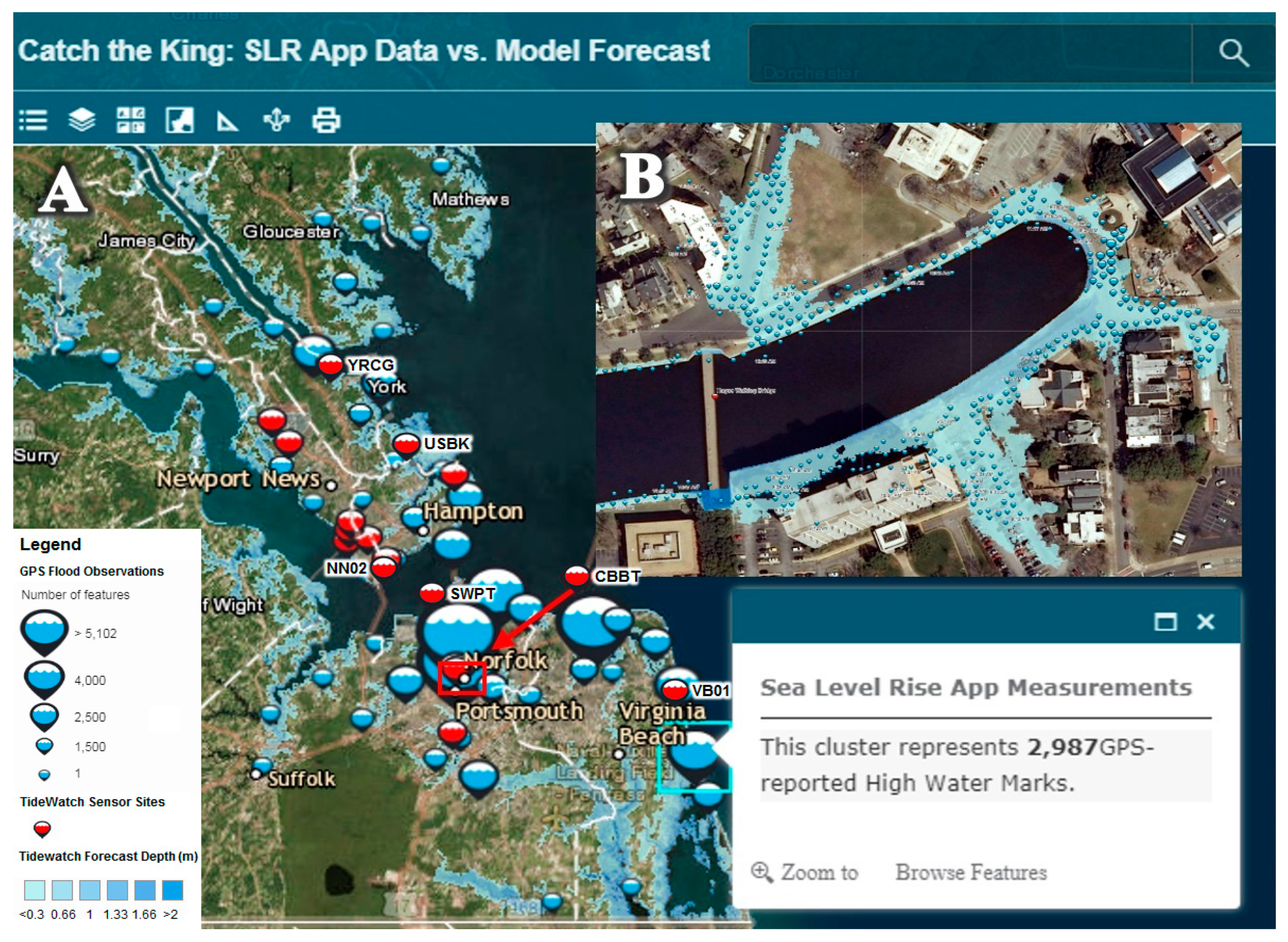
Spatial data collected for each king tide event were aggregated through the Sea Level Rise mobile app and shared online using interactive web maps, so that volunteers with minimal GIS experience could visualize their own GPS observations populate the Tidewatch model’s predictions in near-real time (Figure 6). This level of data accountability implemented an open interaction where users could conduct their own analyses and make their own mean difference calculations through ArcGIS Online’s distance and area measuring tools from their data in a web browser while viewing the public map. This data interactivity spurred high engagement and participation for students involved in STEM research or related educational classes. 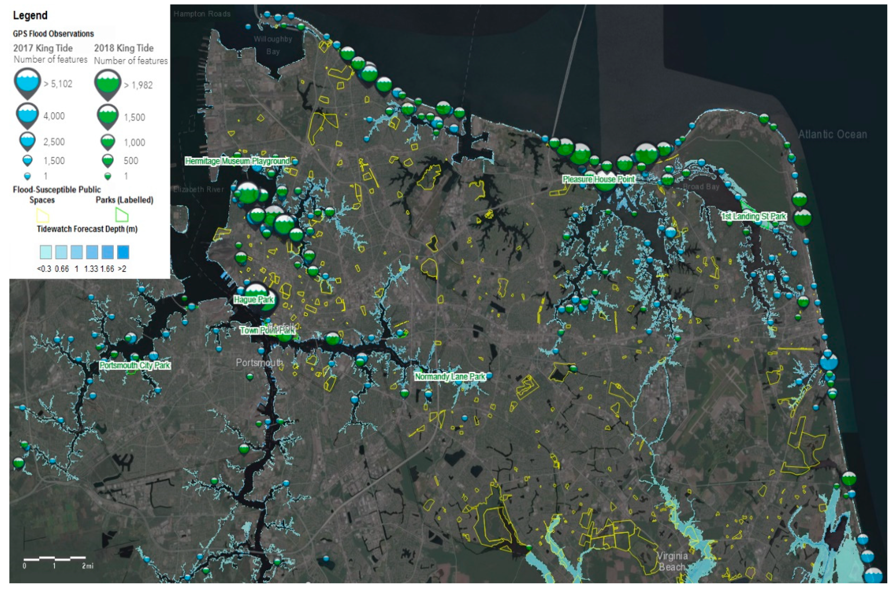Figure 6A shows an aggregated point map of 59,718 high water marks superposed with the Tidewatch Maps throughout the greater Hampton Roads region and showcases the extent of areas not covered by automated sensors that were surveyed through Catch the King in 2017 (

Table 1. A tabulated table of quantities mapped by Catch the King volunteers in coastal Virginia, USA, where the SCHISM-Driven Tidewatch storm tide model provided inundation forecasts.

Year	Distance (Unique km)	Distance (Total km)	GPS Points	Photographs
2017	104.28	416.66	59,718	1582
2018	69.36	277.77	37,728	458
TOTAL	173.64	694.43	97,446	2040

).

Comparatively, 2018 surveyed an even broader area than was monitored in 2017, but with less density (Figure 4). For example, Figure 6B shows Norfolk’s Hague, where thousands of GPS data were collected in both years. In areas where a significant point density is reported, data points can form more than simple flood contours when combined with digital elevation survey data. With sufficient point density, one can form their own observation-driven interpolated flood model for comparison with hydrodynamic simulation results. In this case, the areal extent of The Hague shown in Figure 6B yielded a 94% match with the raster polygon built from the interpolated GPS points, with the Tidewatch model slightly erring on the side of over-prediction. The cursory overview of the Greater Hampton Roads Region shown in Figure 6 shows the Tidewatch Map in blue, GPS citizen science observations as aggregated blue dots, which render and dis-aggregate based upon the zoom level, and water level sensors from the Tidewatch Charts as red dots. This legend theme will persist through the next several spatial comparison figures, and was designated through the Sea Level Rise app for the observation data, and for the model via a meeting of the CCRFR with emergency managers [44].

Given that flood impacts for king tides are simply tidal calibration data that are likely to be aligned along similar elevation contours without intervening atmospheric conditions, linear distance metrics can be useful to compute spatial differences in relatively flat areas. The standard distance formula may then be computed by GIS software to calculate the difference between each GPS data point to the nearest predicted inundated space. To compute this, the modeled geospatial flood depths served through VIMS’ Tidewatch Maps were converted into vector data polygons, with the maximum flood extent representing the 0 m flood contour. As the volunteers were instructed to map inundation in their communities by dropping time-stamped digital GPS breadcrumbs, the citizen scientists’ data should ideally represent the observed GPS flood extents, and in most places, the model had an overwhelmingly favorable agreement. 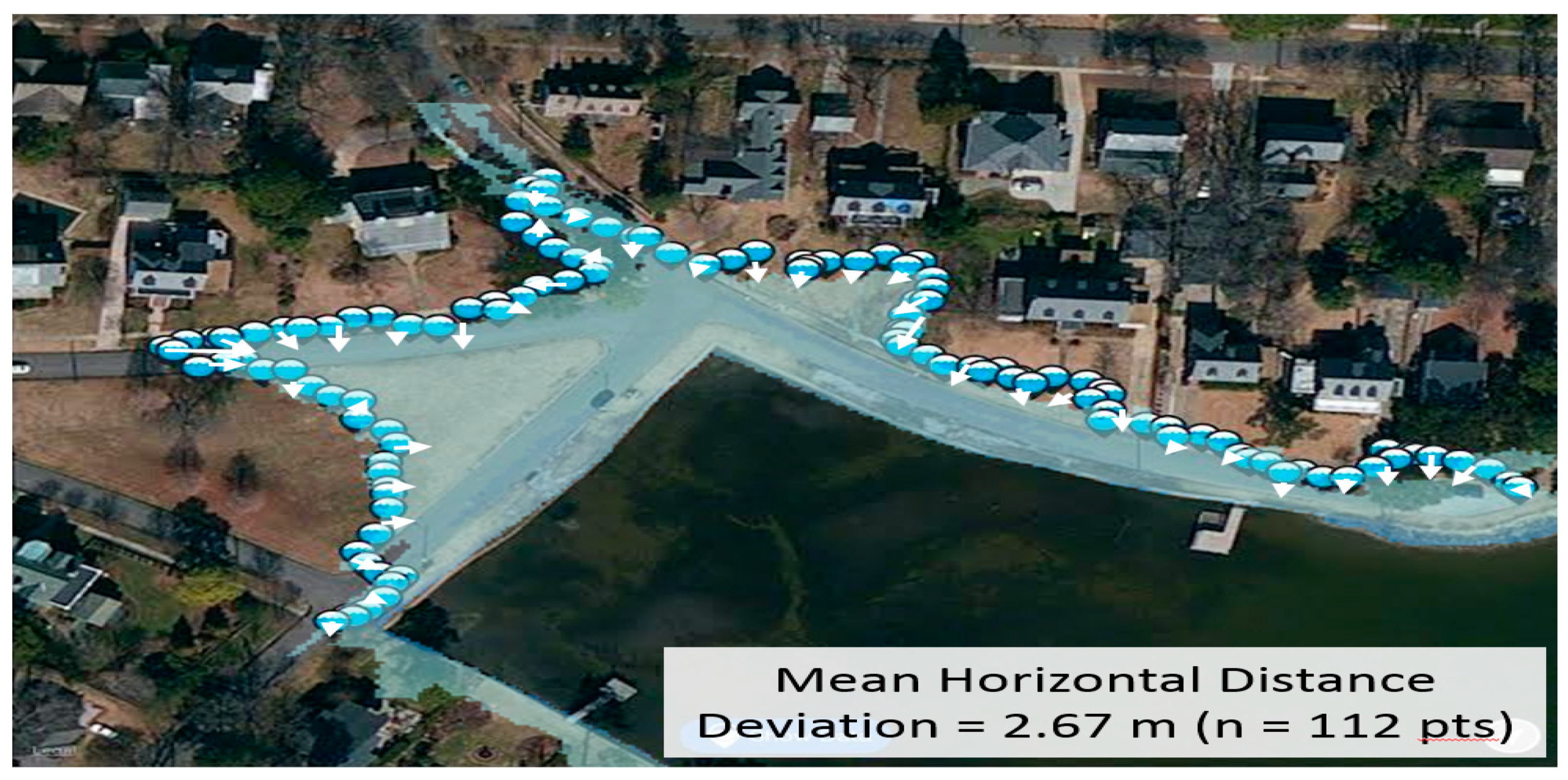Figure 7 shows an example in Norfolk’s Larchmont neighborhood adjacent to a dog park, where flooding is frequent, and the 112 points were used to compare with the light blue modeled flood extents as a linear distance, and averaged to form a mean horizontal distance deviation (MHDD) metric, which yielded an average deviation of 2.67 m for this site during the 2018 king tide.

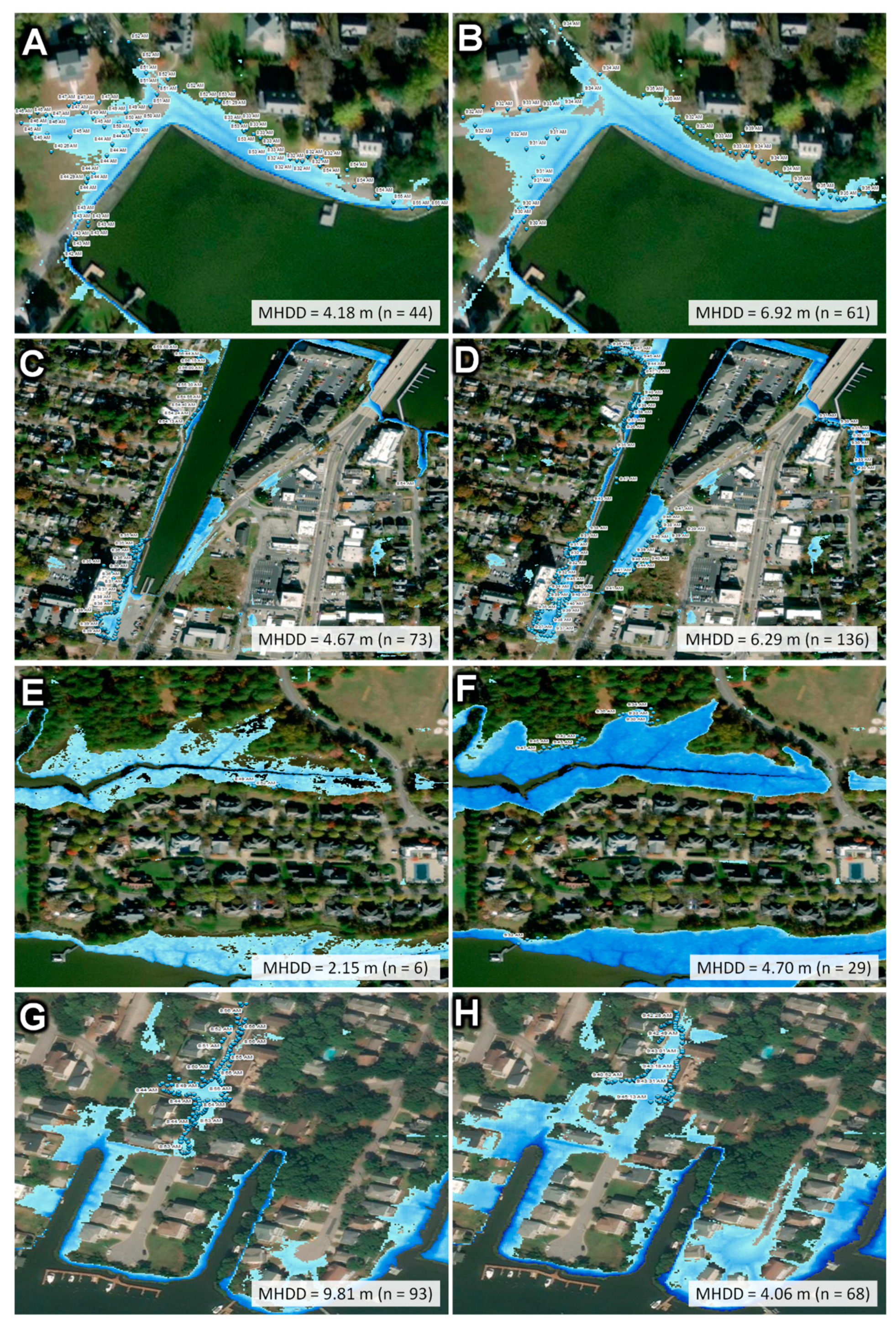
Likewise, several other areas, ranging from residential, commercial, and industrial land uses, during the 2017 king tide are featured in Figure 8. Since Tidewatch Maps provide more than simply a maximum inundation extent, unlike tidal depths estimated from a bathtub model or a sea level rise topographic flood elevation viewer, temporal accuracy can also be assessed through the GPS timestamps reported on each user’s measurements through the Sea Level Rise app. Figure 8A,C,E,G, shows a model distance comparison of forecasts and data from 13:00 to 13:59 UTC. Figure 8B,D,F,H show observation data and model forecasted depths for the same sites an hour later from 14:00 to 14:59 UTC. These figures are used to show varying flooding conditions during the king tide on 5 November 2017, which occurred at 14:30 UTC, similar to those noted in Figure 3 during 2011 Hurricane Irene. Figure 8 shows individual sites where monitoring efforts took place in 2017 and ultimately contribute to the overall figure of +/−5.9 m in horizontal difference between the maximum extents predicted via the Tidewatch Maps and the 59,718 high water marks measured through Catch the King.

Figure 8A shows data from the 2017 king tide for the same area as Figure 7 in Larchmont, Norfolk for 44 high water marks collected by 2 citizen scientists from 13:32 to 13:52 UTC to yield a MHDD = 4.18 m. The same site from an hour later is shown in Figure 8B, comprised of 61 high water marks collected by 1 volunteer from 14:30 to 14:39 UTC to yield a less favorable MHDD = 6.92 m during the peak inundation period in Catch the King 2017. Figure 8C depicts inundation during the 2017 king tide along the south bank of the Lafayette River near the Haven Creek Boat Ramp in Norfolk by 73 high water marks collected by 2 citizen scientists from 13:35 to 13:59 UTC to yield an MHDD = 4.67 m. The same site an hour later is shown in Figure 8D, this time featuring 136 high water marks collected by 3 people from 14:30 to 14:47 UTC to yield a less satisfactory MHDD = 6.29 m during the peak inundation period on 5 November 2017. Figure 8E showcases GPS data from Catch the King 2017 for the Lafayette Shores neighborhood, nestled in the east bank of the Lafayette River, through six high water marks collected by a citizen scientist from 13:49 to 13:52 UTC to yield an MHDD = 2.15 m. The same site from an hour later is shown in Figure 8F, comprised of 29 high water marks collected by 2 people from 14:30 to 14:47 UTC to yield a less favorable MHDD = 4.70 m during the peak inundation period. Figure 8G depicts inundation during the 2017 king tide along the north bank of Little Creek in the East Ocean View neighborhood of Norfolk via 93 high water marks collected by 2 citizen scientists from 13:44 to 13:56 UTC to yield an MHDD = 9.81 m. The same site from one hour later is highlighted in Figure 8H, now featuring 68 high water marks collected by 1 person from 14:40 to 14:45 UTC to yield an improved MHDD = 4.06 m during the peak inundation period during Catch the King 2017.

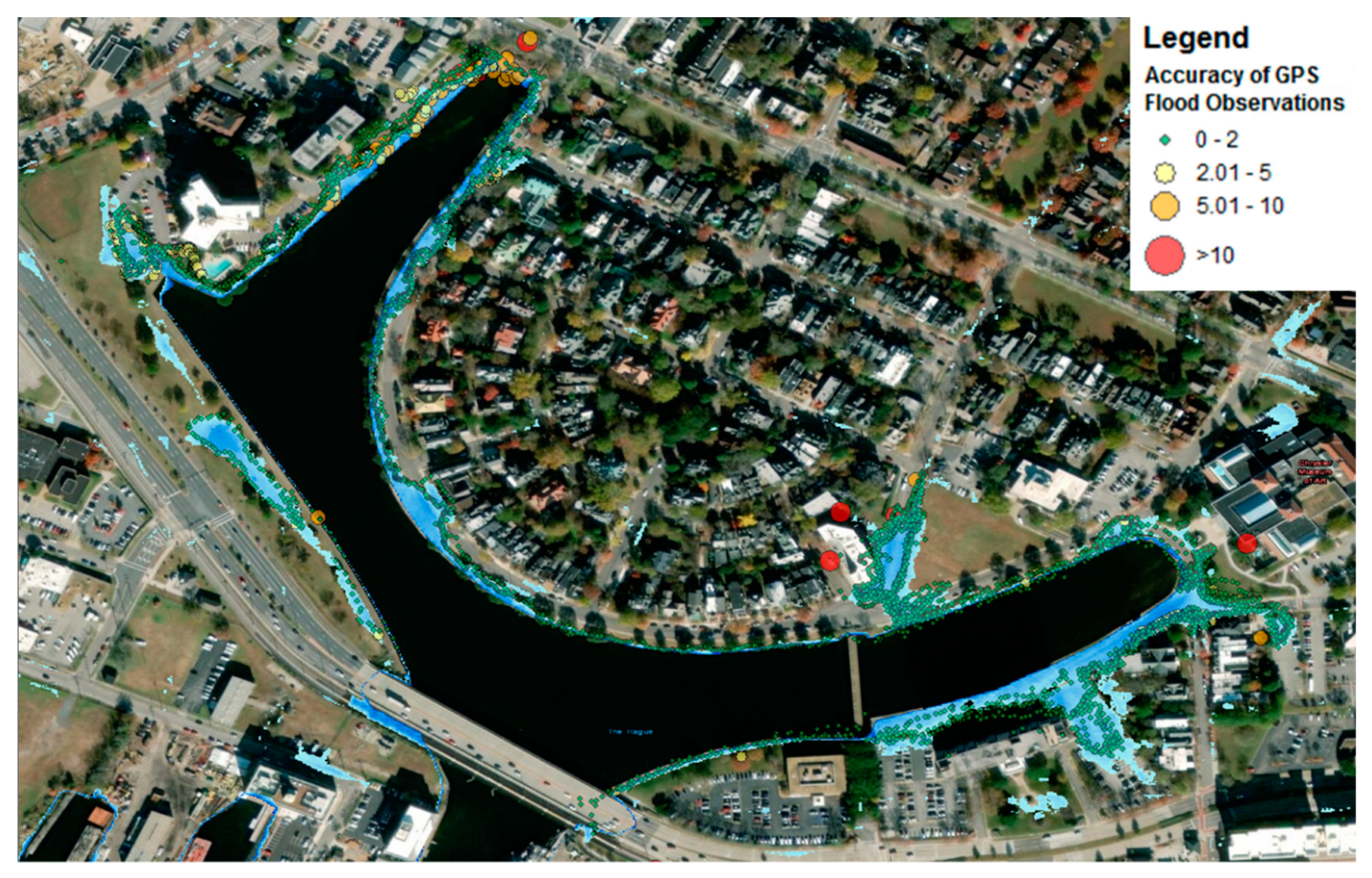
While the areas shown in Figure 8 were surveyed by few citizen scientists, the area shown in Figure 6B is one of the most frequently monitored areas in the Sea Level Rise app’s history. During 2017’s Catch the King, the area featured in Figure 6B was monitored by 27 different volunteers at different times (not all during the flood peak period) to form 27 king tide inundation contours for The Hague. These were mosaicked into a composite maximum extent contour map comprised of 1134 GPS points stretching 2.17 km to form a maximum extent contour for VIMS to compare with its Tidewatch Maps modeled inundation. The total distance walked and recorded using the Sea Level Rise app by all 27 volunteers for The Hague alone in 2017’s Catch the King was 22.58 km (Figure 6B). This is 10.39× the composite’s distance at this king tide inundation site, meaning >10× the actual effort, or about a 10× greater distance was walked than represented by the composite 0 m flood depth contour. As a result, these distances along the waterways that were travelled as effort expended by volunteers was significantly greater than needed to efficiently validate the flooding extents (by 10×), and this is not counting a volunteer’s travel to and from each reported flood site.

For perspective, the grand total for over 1000 volunteers to map inundation distances across both Catch the King years was 631.35 km, with the total number of unique king tide contours travelled in Hampton Roads across both years adding up to 173.65 km (Table 1). Therefore, significantly more effort was used than needed to effectively map the site, with Norfolk’s Hague experiencing the greatest duplicated effort. This was also indicative of overlapping efforts among other high-density monitoring areas at public beaches in Norfolk, Virginia Beach, and Hampton representing the other greatest density GPS data density areas with >6× overlap. As noted previously, the increased density of GPS data proved to be a boon towards supporting the development of data-driven area maps, which was useful in The Hague, but were less useful on public coastal beaches where the water was not surrounded by land, with transient sand elevations that may vary from those embedded in the hydrodynamic model via the latest lidar elevation surveys. Thus, in 2018′s Catch the King, greater emphasis was placed on coordinating volunteers at registration to commit to mapping unique locations when communicating with volunteers via training events, and through print and social media to best value their time commitment and most efficiently validate the model.

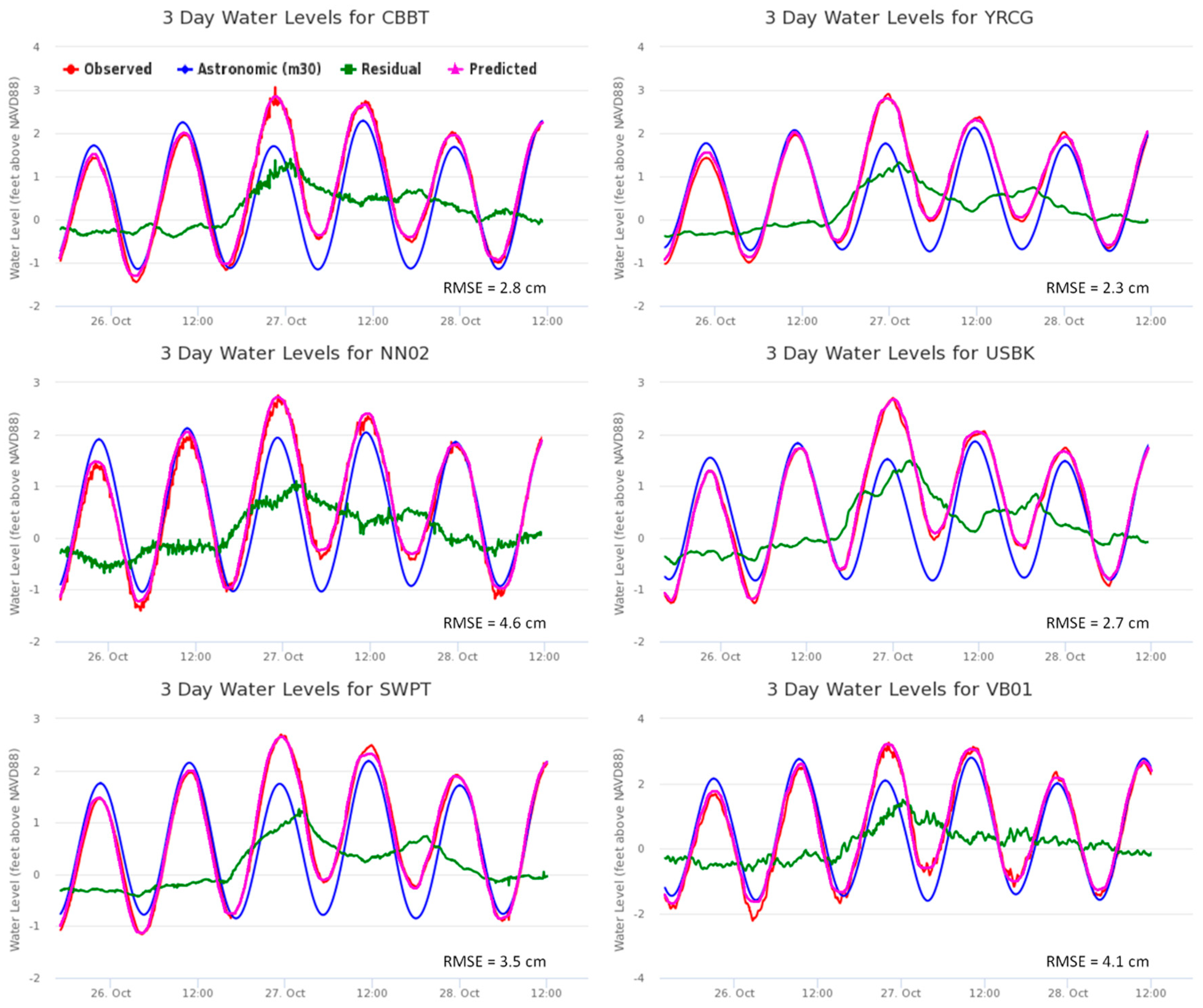
Aside from the horizontal GPS surveys reported through Catch the King, Tidewatch is routinely validated through automated water level monitoring sites. An overview of the water level sensor data extracted from sensors through Tidewatch Charts during Catch the King 2018 across all data points revealed a favorable average vertical accuracy assessment of 3.7 cm via the root mean squared error (RMSE). This metric was drawn from 28 StormSense water level sensors, and 16 tidal USGS Sensors and 4 NOAA sensors. Six of these sensors, including three NOAA, two StormSense, and one USGS sensor, are shown in Figure 9 from VIMS’ Tidewatch Charts, as an example comparison of hydrodynamic model performance during 2018′s Catch the King. These charts from 2018 are labeled in Figure 6A with their four-character station abbreviations, for spatial reference, with their time series data shown in Figure 9.

The region had 16 less water level sensors in 2017, and Catch the King in 2017 took place during a king tide with no additional amplifying wind or rainfall effects. The aggregate RMSE comparison in 2017 across 32 sensors was 3.5 cm, resulting in a slightly better agreement with the model than the 3.7 cm RMSE value reported in 2018 [27,35]. As a result of the “blue sky” conditions, 722 citizen scientists collected data in 2017, but their data was less dynamically interesting than 2018, which had less volunteers (431), due in part to a mild nor’easter that occurred on the night before Catch the King, making the weather less favorable for volunteers. The nor’easter brought 11.17 m/s (25 mph) sustained winds for nearly 3 h from 03:00 to 06:00 UTC on 27 October 2018 (yet contributed negligible rainfall), as seen in the residual fluctuations represented by the green line of each automated monitoring gauge’s measurements in Figure 9.

4. Discussion

As citizen scientists contribute significant amounts of their time to collect these intricate geospatial data sets, care is taken by the custodians of those data to perform quality assurance and quality control on those data before subjecting them to rigorous scientific analysis. The raw volunteer data for each Catch the King survey in 2017 and 2018 were modified after initial statistics were reported to filter out and otherwise minimize bias in this study. This was in an effort to provide the most meaningful model validation statistics, which were reported in the results section, and were honed to validate three important factors for model validation: Duration, depth, and degree of inundation:

Duration

(1)

Points with a reported timestamp more than an hour outside of the time window in which the king tide occurred at that location were not included in the comparison.

(2)

Those points within the window were rounded to the nearest hour to split them into comparative groups for each hourly model output for comparison (as depicted in Figure 8).

Depth

(3)

Surveyed points were merged with the topobathymetric DEM used to build the model, developed by the USGS and published in [45], to append elevation values.

(4)

Any points >0.91 m (3 ft) elevation above the North American Vertical Datum of 1988 (NAVD88) were not included in the model comparison, as the king tide from neither year exceeded this height at any water level sensor in the region (Figure 7).

Degree

(5)

Points with an appended photograph were collected back away from the water’s edge (for land marking and visual perspective), and thus were not included as part of the flood contour comparison. If included, these would over-predict the degree of flooding.

(6)

Points with a radial accuracy metric >10 m (32 ft) were too inaccurate to include, as they misrepresent the degree an area was inundated, favoring over-prediction (Figure 10).

The extent that duration of inundation was addressed and timing of when a flood event will arrive dictates the potential mitigating actions that may be taken. Tidal inundation events can easily be predicted through harmonic algorithms, and hydrodynamic models can improve upon this by informing citizen scientists, community planners, and emergency managers alike when the flood waters will arrive. This information is useful for personal preparation of one’s home and assets that may be in low lying areas, route planning and guidance for personal and emergency response vehicles, and for scheduling road closures to minimize vehicular loss. Figure 4 and Figure 8 illustrate the difference an hour makes in terms of accuracy on model validation, and in the future, the recommendation for more frequent spatial mapping has already been recommended for the future development of Tidewatch Maps to eventually shift to 30 min time steps for the online time-aware layers for depicting more temporally-resolute flood mapping beyond hourly updates. However, presently, Tidewatch Maps are used to map all of Virginia’s coastal floodplain via SCHISM’s model outputs at a 1 to 5 m resolution (depending upon the accuracy of lidar point spacing for the model’s underlying digital elevation assumptions). A 36-h Tidewatch forecast already consists of 37 state-wide coastal flood maps being automatically produced every 12 h. Thus, doubling that number to 72 iterative Tidewatch Maps per cycle is both computationally expensive for the model’s post-processing, and impractical for users loading its flood forecasts via the web without newer technology to enhance loading times. Since users have most frequently accessed Tidewatch Maps using their smart phones to view its flood predictions during periods of significant power and internet outages, greater temporal resolution for 30-min update intervals is not likely to be implemented soon, as additional loading times are even more cumbersome for mobile devices.

Aside from depths being directly validated via amplitude comparisons with automated water level sensors, surveyed points collected through Catch the King were merged with a DEM to translate the collected data to contours. While most modern smart phones have an altitude sensor, its error on accuracy is not sufficient to accurately report flood depths or meaningfully report heights above a reference datum. The Sea Level Rise app does display one’s altitude in the app interface and records this with each point, but not all phone models share these data with the app or possess the internal hardware to report this. Thus, for the most reliable elevations, the GPS high water marks were merged with the topobathymetric DEM used to build the SCHISM model and the Tidewatch Maps, developed by the USGS [45]. Many citizen scientists were likely to test the app before venturing out to collect data, and several data points that were nowhere near water were collected. Instead, these points appeared in houses, apartment complexes, or traced around isolated puddles in parking lots that were non-contiguous with neighboring estuaries. These locations were flagged for use in storm water studies, and removed from this tidal inundation model validation analysis for any points >0.91 m (3 ft) elevation above NAVD88 were not included in the model comparison, as the king tide from neither year exceeded this height at any water level sensor in the region, and there was no significant rainfall (>2 cm) accumulated during or preceding either Catch the King tidal flood mapping event. In other cases, users mapped tidal-connected drainage ditches that became inundated during the king tides and these points were included in the analysis (Figure 11 and Figure 12).

The context through which the degree of inundation was monitored by citizen science data is made more useful through following proper training for data collection and appropriate data filtering. Data were collected by 722 volunteers in 2017 and 431 volunteers in 2018. These data were collected by over 20 different smart phone models, which each vary in terms of relative accuracy due to the number of antennae included in each phone model to aid in triangulation of positional accuracy and for general clarity of cellular broadband communications through the device. As such, citizen science surveys are inherently less precise than those conducted by professional scientists using industry-standard GPS receivers capable of real time kinematics (RTKs). Since the high variation in phone models introduces variable accuracy, as does the number of GPS satellites in range, an estimated radial error metric is reported by the Sea Level Rise app for each GPS measurement by assessing the incoming signals from the global navigation satellite systems along with a correction stream. However, unlike professional survey equipment operated by trained professionals, smart phones are presently unable to achieve the 1 cm positional accuracy that RTK GPS tools can. Thus, points with a radial accuracy metric >10 m were not included in the spatial comparison (Figure 10).

Upon filtering for these three things, it was found that the Tidewatch Map comparisons on 5 November 2017 during Catch the King 2017 had an overall MHDD of 5.9 m (19.3 ft). This statistic was calculated from 57,986 of the 59,718 total high water marks collected after less than 3% of the citizen scientists’ measurements were filtered out for any of the six reasons previously noted for relative error on duration, depth, or degree of flooding. In a similar fashion, comparisons between the high water marks collected by citizen scientists during Catch the King 2018 observed a slightly less favorable overall MHDD of 6.2 m (24.6 ft), likely attributed to the winds from the mild nor’easter that occurred in the hours leading up to the event. This MHDD was calculated from 30,920 of the 33,847 total high water marks collected after 8.6% of the citizen scientists’ measurements were filtered out of the surveyed data.

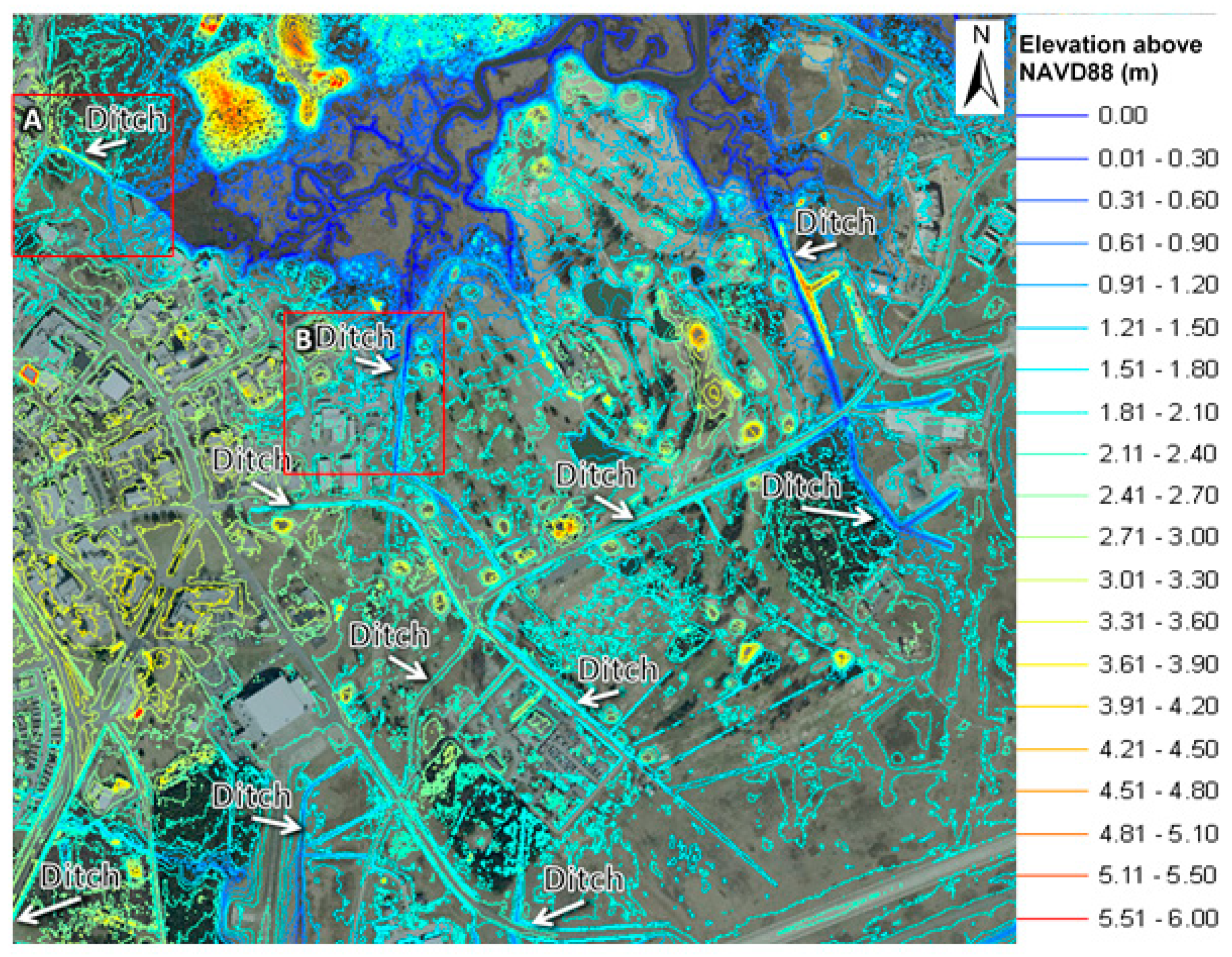
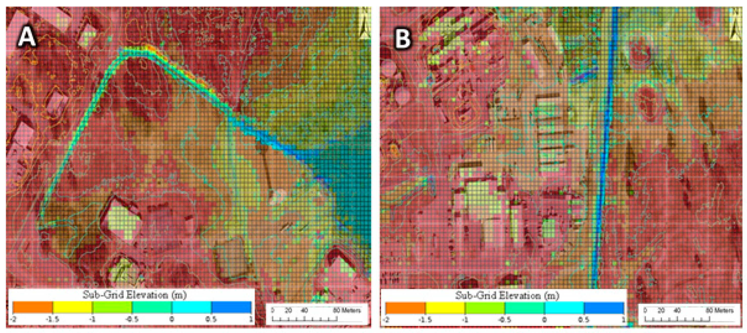
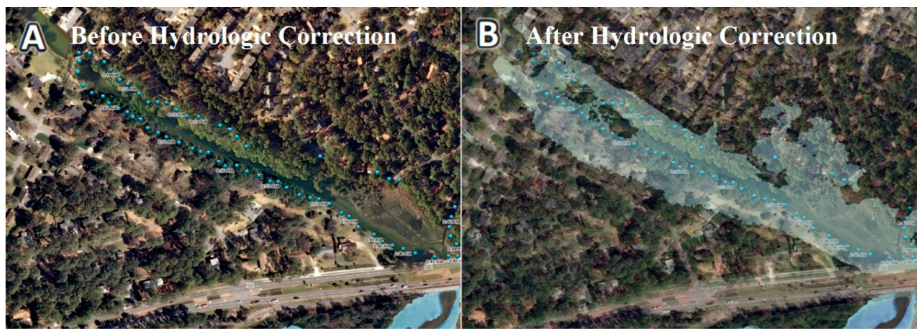
In the interest of improving future forecasts, it was found that less than 1% of the filtered GPS high water marks were still not within 50 m of the Tidewatch Map’s predicted inundation raster. Further investigation into these sites identified two reasons for the discrepancy, both related to errors in hydrologic correction of the model’s DEM calculated water depth assumptions. Figure 11 outlines a series of above-ground drainage ditches in Hampton VA, that occasionally become inundated when the water table rises with extra high tidal waters. Connection through these narrow drainage ditches can be obscured by thick canopied trees adjacent to the narrow tidal creeks and mostly non-tidal ditches that feed those creeks (Figure 12). The model’s elevations are attributed to averaged digital elevations from aerial lidar surveys to source the DEM that the model uses to represent reality. Thus, the depths of the bottoms of these fine scale ditches (<1 m wide) were not likely to be correct unless the point spacing is extremely high. Naturally, this is acceptable, since the model was scaled to (at best) 1 m spatial resolution, and cannot accurately represent the slopes of such detailed drainage features without scaling to a 0.33 m resolution. 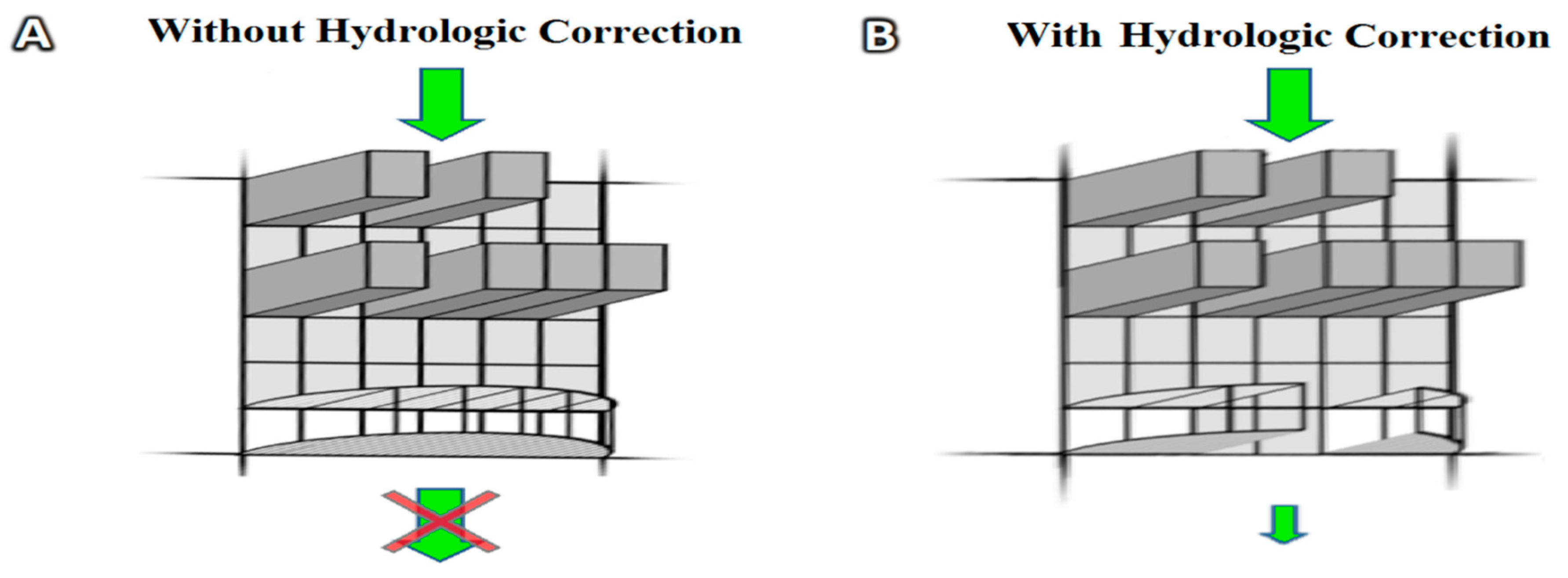Yet, these ditches were found to become tidal conduits for fluid movement capable of causing inundation far from the shoreline during king tides [46]. In other places, bridges over typically non-tidal creeks were not removed from the aerial survey data used to build the DEM, and removal of the occluding feature aided hydro-correction to correct the model’s incorrect volume displacement in areas where entire creeks were shown to be dry due to the artificial dam imposed by a bridge, constricting proper fluid flow (Figure 13). Thus, one of the most important and immediately noticeable achievements that Catch the King accomplished for the hydrodynamic model’s validation was the aid of hydro-correction for several small streams that were obscured in the aerial lidar surveys informing the Tidewatch Maps. In the case of several ephemeral creeks that temporarily became tidal during the king tide, the citizen scientists’ survey identified locations where these ditches needed to be corrected (Figure 14) [47].

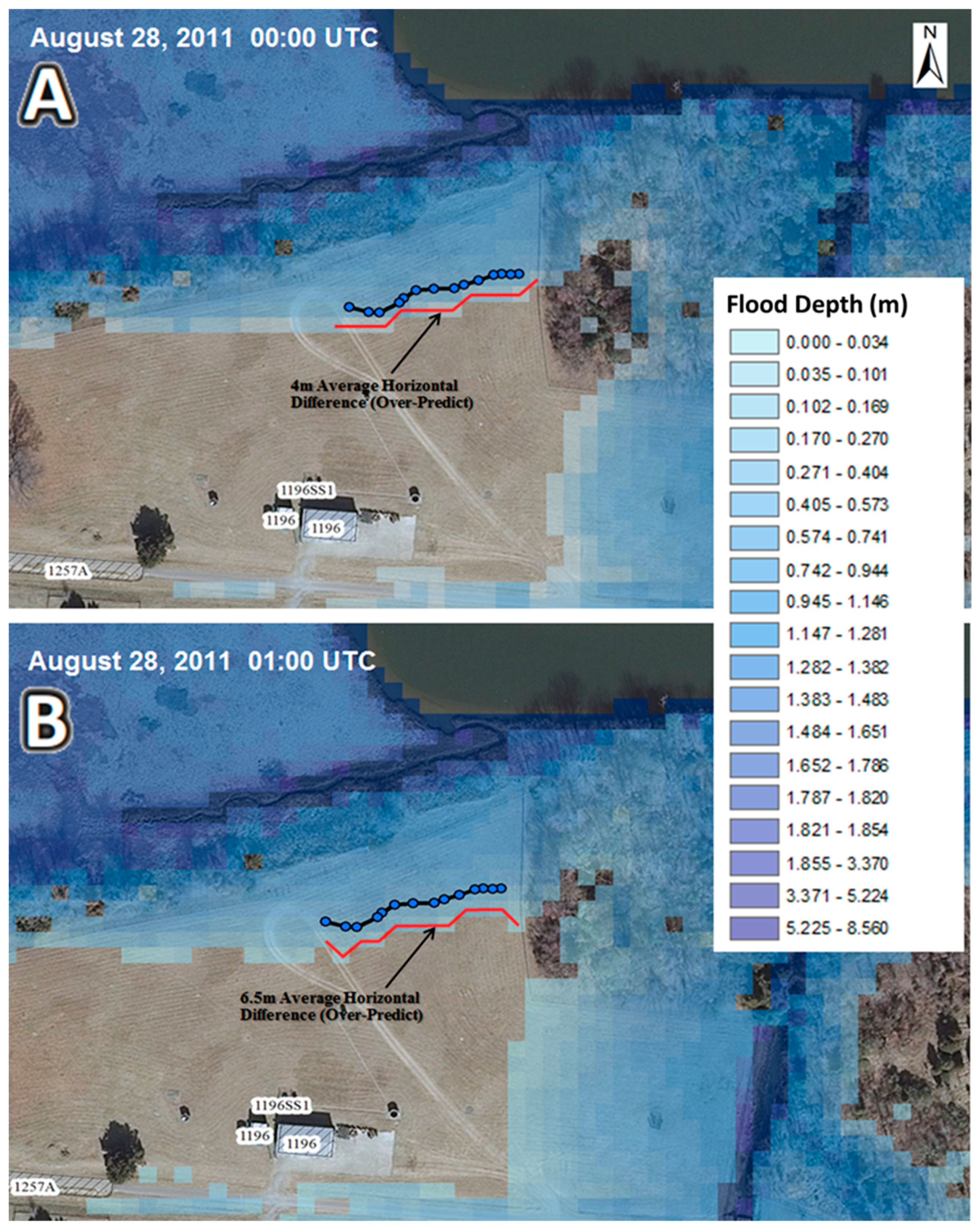
For example, a typically non-tidal creek feeding Wolfsnare Creek in Virginia Beach was inundated during the king tide in 2017. Catch the King volunteers mapped the king tide approximately an hour before the king tide’s peak, and the large initial mean horizontal distance difference from this cluster of points drew researchers’ attention to investigate the hydrodynamic model’s under-prediction of inundation. The error was traced back to a faulty elevation assumption attributed to obstructed flow underneath a bridge. VIMS researchers hydro-corrected the landscape to open flow using neighboring elevations from the DEM through the box culvert underneath the bridge and corrected ground elevations impacted by thick tree canopies surrounding a creek bed with low aerial lidar-point-spacing.

5. Conclusions

A large-scale flood monitoring citizen science data collection effort was used to favorably validate an automated browser-based flood mapping service driven by a cross-scale hydrodynamic model predicting storm tide inundation in coastal Virginia, USA. The operational modeling effort for predicting tidal flooding can be mapped using multiple methods, yet the most effective method was found to be the automated implementation of a street-level hydrodynamic model. The Tidewatch Maps implemented by the Virginia Institute of Marine Science (VIMS) leveraged their SCHISM hydrodynamic model with inputs of: atmospheric wind and pressure data, tidal harmonic predictions at the open boundary, and prevailing ocean current inputs, such as the Gulf Stream. This information was successfully computed from a large scale model and translated to the street-level via SCHISM’s computationally efficient non-linear solvers, and semi-implicit numerical formulations aided by a sub-grid geometric mesh with embedded lidar elevations.

Validation in the vertical scale found that the SCHISM model outputs via the Tidewatch web mapping platform compared well in Hampton Roads among the 32 extant water level sensors during the highest astronomical tide of the year on 5 November 2017, a king tide, yielding an aggregate RMSE of 3.5 cm. The region expanded its sensor base to 48 through an IoT sensor project, StormSense, to compare well again during the king tide on 27 October 2018, resulting in an RMSE of 3.7 cm. Horizontal validation was aided by time-stamped GPS flood extent data collected by citizen scientists through the world’s largest environmental survey (in terms of the most contributions in the least amount of time), Catch the King. The citizen science flood mapping survey was established in Hampton Roads in 2017 and recruited volunteers through local, print, and social media outlets. The survey’s organizers then trained the citizen scientists in the use of the free Sea Level Rise mobile flood mapping application at frequently inundated public spaces in the months leading up to each king tide event.

The citizen scientists’ flood monitoring data formed time-indexed GPS breadcrumbs to form contours that were successfully aggregated and compared with the maximum inundation extents of the same time interval from VIMS’ Tidewatch Maps. The data were filtered to minimize bias attributed to errors related to observing flooding duration, depth, and degree. Once the Catch the King survey data were filtered for these three things, it was found that the Tidewatch Map comparisons on 5 November 2017 had an overall mean horizontal distance difference of 5.9 m (19.3 ft). The model comparison with the observations collected during the king tide on 27 October 2018 were found to be less favorable, yielding an average distance deviation of 6.2 m (24.6 ft), likely attributed to the winds from the mild nor’easter that occurred in the hours leading up to the event. In each spatial validation effort, less than 9% of the surveyed data were excluded from the analysis.

Lessons learned from citizen science surveys have improved the model through cost-effective hydrologic correction of mission conduits for fluid flow. These were identified by filtered GPS observations that the model missed in its initial automated forecast, but were corrected in hindcast, in preparation for the next significant inundation event. Errors in hydro-correction did not relate to errors in friction parameterization of the model, but were more associated with flow pathways that were occluded from aerial lidar surveys. These areas included bridges, culverts, and stormwater drainage systems without tidal backflow prevention valves, which formed artificial dams in the digital surface model embedded in the forecasted Tidewatch Maps. Many of these identified areas have been corrected and have recently been used alongside the successful model validation in Hampton Roads to expand the forecast area of the Tidewatch Maps beyond southeast Virginia to include the entire coastal zone of Virginia in 2019.

As king tides are currently simply nuisance floods, which primarily inundate streets and driveways without significantly damaging infrastructural assets, the issues are presently geared towards traffic and transportation issues. Common concerns from citizen scientists involved in the Catch the King mapping events involved concerns regarding whether their vehicle could be safely street parked or if their vehicles needed to be safely moved into a garage during king tides. Others questioned whether they should take an alternate route to work or school or the store due to potential street flooding. As technology progresses, these questions will become more prevalent as we aim to ascertain whether modern route guidance mobile applications will be intelligent enough to account for intermittent inundation, or unintentionally lead vehicles down flooded streets simply because there is no traffic detected on them while an adjacent elevated street is congested. Some navigation applications, such as Waze, have aimed to crowdsource all road hazard data through their “Connected Citizens” program, but this method is only a temporary solution, as a model cannot currently automate road hazard flags for flooded locations where those particular app users are not or have not logged data.

Naturally, adeptly answering these questions becomes increasingly difficult once self-driving vehicles are involved. Thus, the outcomes of inundation modeling efforts for this tidal calibration effort will more significantly be realized once this trained citizen scientist army is deputized into post-hurricane surveys. Since 2011 Hurricane Irene was the last hurricane to significantly impact Virginia’s Hampton Roads region, the Tidewatch automated mapping model has yet to demonstrate widespread accuracy amidst a significant inundation event since the Sea Level Rise app’s advent in 2014. The goal is to continue to improve the model with each Catch the King tidal calibration and train volunteers so they will be aware of where to find the latest flood forecast information, and how to collect meaningful flood validation data. Thus, this monitoring coordination approach with hydrodynamic modeling provided a novel procedural release of information to depict predicted maximum inundation extents for expediently effective model validation through the use of an overwhelming quantity of quality event data with relatively low risk to volunteer citizen scientists.