Oil Spill Scenarios in the Kotor Bay: Results from High Resolution Numerical Simulations

Abstract

A major threat for marine and coastal environment comes from oil spill accidents. Such events have a great impact on both the ecosystem and on the economy, and the risk increases over time due to increasing ship traffic in many sensitive areas. In recent years, numerical simulation of oil spills has become an affordable tool for the analysis of the risk and for the preparation of contingency plans. However, in coastal areas, the complexity of the bathymetry and of the orography requires an adequate resolution of sea and wind flows. For this reason, we present, to the best of the author’s knowledge, the first study on the subject adopting Large Eddy Simulations for both the low-atmosphere and sea dynamics in order to provide highly-resolved marine surface current and wind stress to the oil slick model, within a one-way coupling procedure. Such approach is applied to the relevant case of Kotor Bay (UNESCO heritage since 1979), in Montenegro, which is a semi-closed basin surrounded by mountains that is subject to an intense ship traffic for touristic purposes. Oil spill spots are tracked along ship paths, in two wind scenarios.

1. Introduction

Oil spill accidents represent a major threat to marine and coastal environment, impacting both biological species and human health, as well as economic, touristic and commercial activities. For example, according to data collected from 1977 to 2003 about 304,700 tons of oil have been released in the Mediterranean Sea mainly due to extensive marine traffic of oil tankers and ships [1,2].

Weather conditions, oil physical and chemical characteristics determine oil fate and persistence at sea. Most kinds of oils spread on the sea surface as a thin film, the slick is then driven by the sea currents and wind stress; furthermore, if the oil temperature drops below the pour-point, oil can solidify and form tar balls. In case of wavy and turbulent seas, small oil drops can detach from the oil slick and then, depending on their density, particles can either sink, float on the surface or be transported along the water column. Moreover, oil interacts with the surrounding environment. Immediately after spills, oil can evaporate and, under the action of wind and waves, it can absorb water droplets producing emulsion. Such phenomena, called weathering processes, change oil physical and chemical properties in time, strongly affecting oil fate and persistence at sea [3,4,5,6].

Given the significant impact of oil spill on the environment and economy of the area, over the years, efforts have been devoted to the preparation of contingency plans, aimed at ensuring fast response and to facilitate clean-up operations after accidents. In this context, oil spill numerical models have been widely established as helpful tools, both for development of contingency plans and for guiding clean-up operations. Oil slick models are usually integrated with hydrodynamic and meteorological models that provide sea currents and wind data. The modeling approaches can be classified as Lagrangian, Eulerian and Lagrangian/Eulerian hybrid models [4,7]. In the Lagrangian models, e.g., [2], oil slick is treated as a multitude of finite size particles, which are advected by a mean drift velocity plus a fluctuating turbulent component, the latter usually parametrized by means of a random walk technique. In the Eulerian method, e.g., [8], oil slick dynamics are derived from mass and momentum conservation equations. Finally, in hybrid Lagrangian/Eulerian models (see, for example [9]), a large number of particles parametrizes the oil slick immediately after the spill, and, as far as the width of the slick reaches a terminal value, the computation switches to a Eulerian model.

In the present paper, we study the case of a hypothetical oil spill accident due to ship collision in Boka Kotorska Bay, a long and tortuous fjord situated in the Adriatic Sea. The study is aimed at preparation of contingency plans for the area under investigation. This area is under the UNESCO protection since 1979, for its own important natural and historical heritage. The prevention from possible hazardous situations is becoming urgent in light of the increased maritime traffic over the recent years. To make the study as realistic as possible, the typical ship path is considered within the bay [10,11] in conjunction with oil spill spots identified as dangerous from an environmental point of view.

We use a novel approach to simulate oil slick dispersion in coastal areas characterized by surface currents and low atmosphere circulations governed by complex bathymetry, coastline and orography. We use a two-dimensional Eulerian model derived by Nihoul’s theory [12,13,14] for the oil slick. The oil slick simulation is coupled with LESCOAST [15,16], a high resolution hydrodynamic model used to simulate water circulation in coastal areas. Given the complex orography surrounding the bay, a preliminary low-atmosphere wind simulation is required to take into account the horizontal variability of wind stress. This latter is the main forcing item driving both the oil slick and the sea current in the upper layers, and it has to be properly modeled, for example as suggested in [17].

The paper is organized as follows: in Section 2, we provide a brief overview of the hydrodynamic models for water and air domains; then, we introduce the oil spill model and finally we briefly describe the features of the area under investigation along with the boundary and initial condition for the simulations. Results of the most significant scenarios are reported and examined in Section 3. Finally, the discussion is provided in Section 4.

2. Materials and Methods

In this section, we describe the methodology used for the study: in Section 2.1, we provide a brief description of the LESCOAST/LESAIR model used for the marine and low-atmosphere simulations; in Section 2.2, we present the oil spill model for the analysis of pollutant dispersion; in Section 2.3, we give a description of the Boka Kotorska Bay; in Section 2.4, we discuss the set-up of the simulations.

2.1. Hydrodynamical Model

LESCOAST/LESAIR model [18,19] solves the filtered form of three-dimensional, non-hydrostatic Navier–Stokes equations under the Boussinesq approximation along with the transport equations for scalar quantities, i.e., salinity and temperature/humidity and temperature in marine/atmosphere simulations, respectively.

The LESCOAST/LESAIR model uses a Large Eddy Simulation approach to parametrize turbulence, and the variables are filtered by a low-pass filter function represented by the size of the cells. The subgrid-scale fluxes (SGS), which come out from the filtering operation, are parametrized by a two-eddy viscosity anisotropic Smagorinsky model developed in [18]. Such method is effective in simulating coastal flows on sheet-like anisotropic computational grids.

The complex geometry, which usually characterizes harbor and coastal areas, is treated using an Immersed Boundary Method (IBM), based on a direct forcing approach, as described in [20]; the technique is used to reproduce coastline, anthropogenic structures, bathymetry and topography.

The filtered Boussinesq form of the Cartesian Navier–Stokes equations reads as follows:

Continuity equation:

$$\frac{\partial {\overline{u}}_j}{\partial x_j}=0,$$

(1)

Momentum equation:

$$\frac{\partial {\overline{u}}_i}{\partial t}+\frac{\partial {\overline{u}}_i{\overline{u}}_j}{\partial x_j}=-\frac{1}{{\rho }_0}\frac{\partial \overline{p}}{\partial x_i}+\nu \frac{{\partial }^2{\overline{u}}_i}{\partial x_j\partial x_j}-2{ϵ}_{ijk}{\mathsf{\Omega }}_j{\overline{u}}_k-\frac{\Delta \rho }{{\rho }_0}{g}_i{\delta }_{i3}-\frac{\partial {\tau }_{ij}}{\partial x_j},$$

(2)

Scalar transport equation:

$$\frac{\partial \overline{s}}{\partial t}+\frac{\partial {\overline{u}}_j\overline{s}}{\partial x_j}=k^s\frac{{\partial }^2\overline{s}}{\partial x_j\partial x_j}-\frac{\partial {\lambda }_j^s}{\partial x_j},$$

(3)

where ’−’ represents the filtering operation, $u_i$ represents the ith-component of the Cartesian velocity vector $(u,v,w)$, $x_i$ represents the ith-component of the Cartesian coordinates $(x,y,z)$, t is time, ${\rho }_0$ is the reference density, $\overline{p}$ is the hydrodynamic pressure, $\nu$ is the kinematic viscosity, ${ϵ}_{ijk}$ is the Levi–Civita tensor, ${\mathsf{\Omega }}_i$ is the ith-component of the Earth rotation vector, $\Delta \rho$ is the density anomaly, $g_i$ is the ith-component of the gravity vector, and ${\tau }_{ij}$ is the SGS stress tensor which comes from the nonlinearity of the advective term, $\overline{s}$ is a scalar quantity (e.g., temperature and salinity/humidity), $k^s$ is scalar diffusivity and ${\lambda }_j^s$ is the SGS scalar flux.

In the present low-atmosphere simulations, density variations are small and therefore buoyancy effects are neglected. In the marine simulations, we solve the transport equation of the scalar quantities, temperature T and salinity S, respectively. The fluid density is computed through the state equation:

$$\frac{\Delta \rho }{{\rho }_0}=\frac{\rho -{\rho }_0}{{\rho }_0}=-{\beta }^T(T-T_0)+{\beta }^S(S-S_0),$$

(4)

where ${\rho }_0$ is the reference density at the temperature $T_0$ and salinity $S_0$; ${\beta }^T$ and ${\beta }^S$ are respectively the coefficient of temperature expansion and haline contraction.

At immersed boundaries, we apply the wall-layer model (IBWLM) presented in [21]; and at the open boundaries the Orlanski boundary condition is enforced [22], and it reads as:

$$\frac{\partial {\overline{u}}_i}{\partial t}+C_i\frac{{\overline{u}}_i}{\partial x_i}=0,$$

(5)

where $C_i$ is the phase velocity, calculated as the flux at the cell face.

The effect of the wind imposed over the free surface is taken into account by means of the formula proposed in [23]. It calculates the stress at the sea surface as:

$${\tau }_w={\rho }_a{C}_{10}{U}_{10}^2,$$

(6)

where ${\rho }_a$ is the density of air and $C_{10}$ is the drag coefficient which is a function of wind speed as:

$$C_{10}=(0.8+0.065U_{10}){10}^{-3},$$

(7)

where $U_{10}$ is the wind velocity 10 m above the mean sea level, which is provided by the low-atmosphere simulations.

For scalar quantities, we apply a no-flux condition at solid walls and, at the surface; at the open boundaries, the Dirichlet condition is enforced with values interpolated from measured data.

Equations (1)–(3) are integrated using the finite difference semi-implicit fractional step method of [24]; it is second-order accurate in both space and time. The model adopts a non-staggered grid, meaning that the primitive variables, like velocity, pressure and scalars are located at the cell centroids, while the fluxes are defined at the cell faces. More details about the numerical model can be found in [18]. In [15], the LESCOAST model is validated against measured and numerical results.

2.2. Oil Spill Model

LESOIL [13,25] is a two-dimensional Eulerian numerical model which simulates the main physical processes governing oil behavior at sea from the start of the release for a time period of the order of 24 h. The processes are: transport and spreading under gravity, friction and Coriolis forces, and the short-term weathering processes, namely evaporation and emulsification.

The model, derived from Nihoul’s theory [12], considers oil slick as a thin-film, whose evolution is driven by gravity and friction forces. The equation that is solved for the thickness of the oil slick h reads as:

$$\frac{\partial h}{\partial t}+\frac{\partial v_{j}h}{\partial x_j}=Q+\frac{\partial }{\partial x_j}\left(\frac{\alpha \partial h}{\partial x_j}\right),$$

(8)

where v is the transport velocity induced by sea currents and wind stress; Q is the source/sink term that takes into account a continuous release of oil, or oil loss due to dispersion of particles or evaporation. The term $\alpha =g{h}^2({\rho }_w-{\rho }_o){\rho }_o/0.02{\rho }_w$ can be interpreted as the oil slick diffusion coefficient and it depends on gravitational acceleration g, oil and water densities (respectively ${\rho }_o$ and ${\rho }_w$). Based on literature findings [8], the contribution of sea current and wind stress on the transport velocity of oil slick is given by:

$$v=u_c+k_w{U}_{10},$$

(9)

where $u_c$ is the velocity induced by current which is provided at each time step by the LESCOAST model; $k_w$ is the wind drift factor, set equal to $0.03$ in agreement with relevant literature [8,9,26,27,28]; $U_{10}$ is supplied by the low-atmosphere simulation.

Immediately after the spill, weathering processes can take place, changing oil density and volume, and eventually influencing oil slick fate and persistence. The model can take into account the main processes, namely evaporation and emulsification, by means of established literature models [29,30]. Parametrization of these effects, in Eulerian models, requires an average of quantities, such as wind velocity, over the whole surface/volume of the slick. This approach is suitable for simulating oil slick in an open ocean scenario where wind stress is almost constant, but it is not properly suited for a slick undergoing a highly varying wind-sea current flow conditions. For these reasons, in this study, the weathering processes are not considered. Although this assumption may appear less realistic, it is still reasonable over a time scale of the order of 12 h and it allows for underlining the spreading mechanism due to the combined wind and sea currents’ actions.

In order to facilitate coupling with LESCOAST, the oil model Equation (8) is run on a surface mesh that perfectly matches the horizontal discretization of the first cells layer at the free surface of the marine model. We use a second-order Adams–Bashfort scheme to integrate numerically Equation (8), the diffusion terms are treated using a centered second-order finite differences method, while the advective terms are discretized using SMART, a third order accurate, monotonic scheme [31]. Compared to literature results [8], the method is proved to be accurate without appreciable numerical diffusion [13,25]. At the immersed bodies, we apply a no-flux condition, neglecting the phenomenon of oil deposition over coastlines.

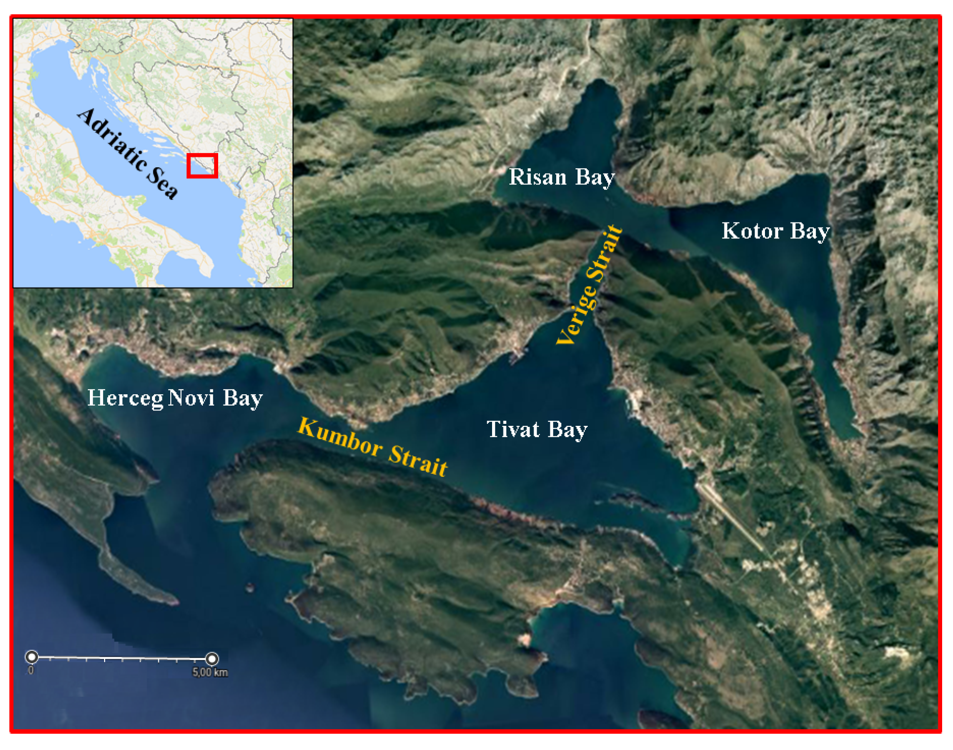
2.3. Kotor Bay Area Description

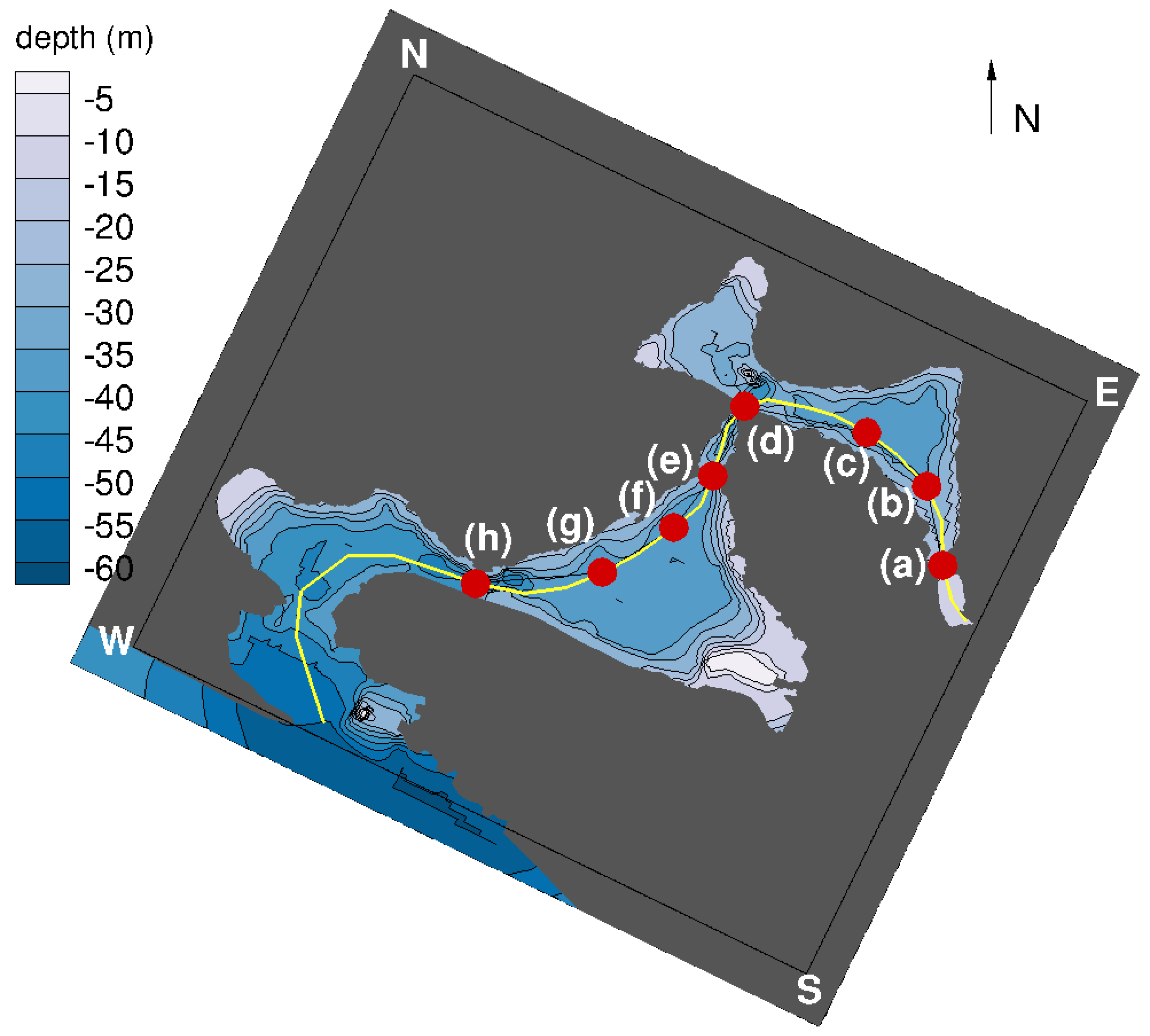
The area under investigation, illustrated in Figure 1, is Boka Kotorska Bay, or Kotor Bay, a semi-enclosed karstic basin situated in the southeastern side of the Adriatic Sea (Montenegro). The bay covers an area of about 87 km${}^2$. The fjord consists of three different sub-bays: Kotor-Risan Bay, Tivat Bay and Hergeg-Novi Bay. The inner one, Kotor-Risan Bay, is further divided into two smaller basins: Kotor Bay (southeast) and Risan Bay (northwest). Two straits connect the three bays: the Kumbor Strait links Tivat Bay with Herceg-Novi Bay, and a narrow canyon, Verige Strait, connects Tivat with Kotor-Risan Bay. The bathymetry decreases rapidly up to a depth of 40 m in the largest part of the basin, the average depth and the maximum depth are 27.3 m and 60 m, respectively. The largest and narrowest widths of the bay are respectively 7 km and 0.3 km [32,33,34].

Numerous fresh water inputs characterize the bay, such as submarine springs, precipitations and rivers. In the upper layers, the water circulation is driven mainly by wind, tide, river runoff, and density gradients; denser water from the Adriatic Sea flows into the bay in the bottom layer. The fresh water inflow mainly impacts the inner bay and, as a matter of fact, salinity at the sea surface increases moving from Kotor-Risan Bay towards the outer basin. In the winter season, characterized by higher precipitations and river runoff, the saline vertical stratification can be more pronounced. One of the most frequent wind conditions for this area is Bora, a strong katabatic wind which flows from the first quadrant. Bora is more frequent in winter time, and it can last for 3–7 days [33,34]. Because of the mountains surrounding the bay, the fetch is small, preventing the generation of significant waves [32]; for this reason, we neglect the effect of waves on sea current and oil slick simulations.

2.4. Case Set-Up

The computational domain for sea circulation has overall dimensions of $L_x=18,435$ m, $L_y=21,575$ m, and $L_z=72$ m. The computational domain is Cartesian and it is discretized uniformly by $640\times 1024\times 24$ grid cells, respectively, with dimensions of about $\Delta x\approx \Delta y\approx 25$ m and $\Delta z\approx 3$ m. The coastline, the anthropogenic structures and bathymetry, as well as topography for the low-atmosphere simulation, are reproduced by the IBM [20]. The computational grid is illustrated in Figure 2; the black rectangle identifies grid borders, and its four corners are labelled with Cardinal points according to grid orientation. The immersed body used to reproduce the coastline is shaded in dark-gray, while the contour colors represent the depth of sea bottom as reproduced in the computational domain. On the southwest side, the basin exchanges water with the Adriatic Sea. 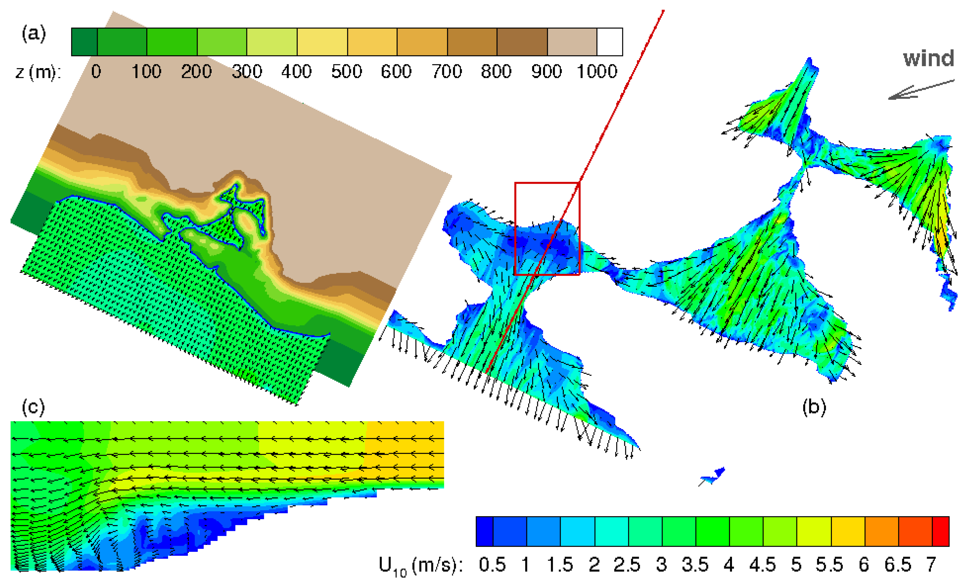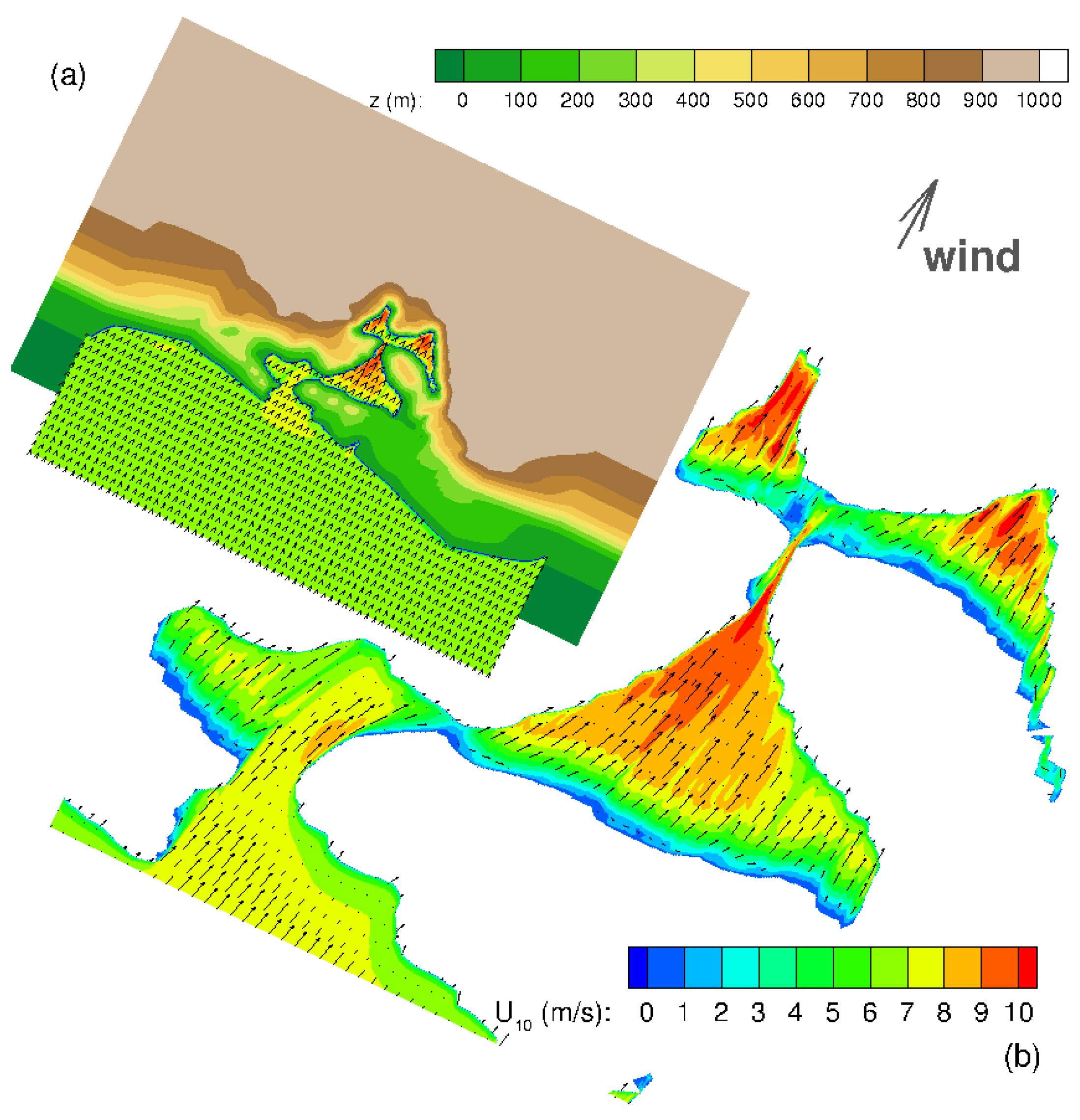Here, we apply the Orlanski boundary condition (Equation (5), [22]), which allows for the simulation of the inversion of the currents over the vertical. At the sea surface, currents are forced by wind stress, whose intensity and direction are obtained by LESAIR Simulations (LAS).

For the low-atmosphere, first, a simulation was run on a large and coarse grid (hereafter referred to as LASc); then, the obtained velocity data were nested as initial and boundary conditions of a second simulation on a smaller and finer grid (hereafter labeled as LASf). The height of the domain ($L_v=2000$ m) is the same for both low-atmosphere grids, and it is discretized by 24 grid cells, stretched in order to obtain a finer resolution near the surface. For LASf, the horizontal domain dimension and discretization are the same as those adopted for the marine domain, while, for the LASc, the horizontal dimensions of the domain are three times larger than in LASf, retaining the same number of grid points.

For the atmosphere simulations, two summer-wind conditions are chosen: the first is the Bora wind case, which is the most frequent wind in the area; the second is the Libeccio (southwest) wind condition. Although it is not the most frequent wind in the area, it is chosen because it represents the worst scenario in case of oil spills, especially in low river runoff conditions. Libeccio, blowing inland from the Adriatic Sea, prevents oil slicks from flowing out of the bay.

The boundary conditions applied for the LASc are: a logarithm inflow velocity with intensity $U_{10}=6$ m/s, set at the wind side (northeast for Bora wind simulation $\theta =65$° and southwest for Libeccio wind simulation $\theta =206$°), named Log Inflow in

Table 1. Summary of boundary conditions applied.

	LASc Bora	LASc Libeccio	LASf	Sea sim.
Top	Free Slip	Free Slip	Free Slip	Wind stress Equation (6)
Bottom	Free Slip/IBWLM	Free Slip/IBWLM	Free Slip/IBWLM	IBWLM
Side N-E	Log Inflow:	Orlanski Outflow	Nesting	Ibm
	$U_{10}=6$ m/s,	Equation (5)
	$\theta =65$°N
Side S-E	Periodic	Periodic	Nesting	Ibm
Side W-S	Orlanski Outflow	Log Inflow:,	Nesting	Ibm/Orlanski Outflow
	Equation (5)	$U_{10}=6$ m/s
		$\theta =206$°N
Side N-W	Periodic	Periodic	Nesting	Ibm

BM = Immersed boundary method; IBWLM = Wall Layer Model for Immersed boundary.

. On the opposite sides, southwest and northeast for Bora and Libeccio cases, respectively, the Orlanski boundary condition is adopted. On the northwest and southeast sides, periodicity is enforced. On the top boundary, we use a free slip condition. On the bottom boundary, at the interface with the sea, a free slip is used, while, at the immersed boundaries surface, a wall model is applied. The LASf boundaries and initial conditions are provided by a nesting procedure, interpolating data from the coarser simulation. Finally, from the computed wind velocity 10 m above the surface, the stress at the free surface of the hydrodynamic model is calculated using Equation (6). The summary of boundary conditions applied for air and sea simulations is reported in Table 1.

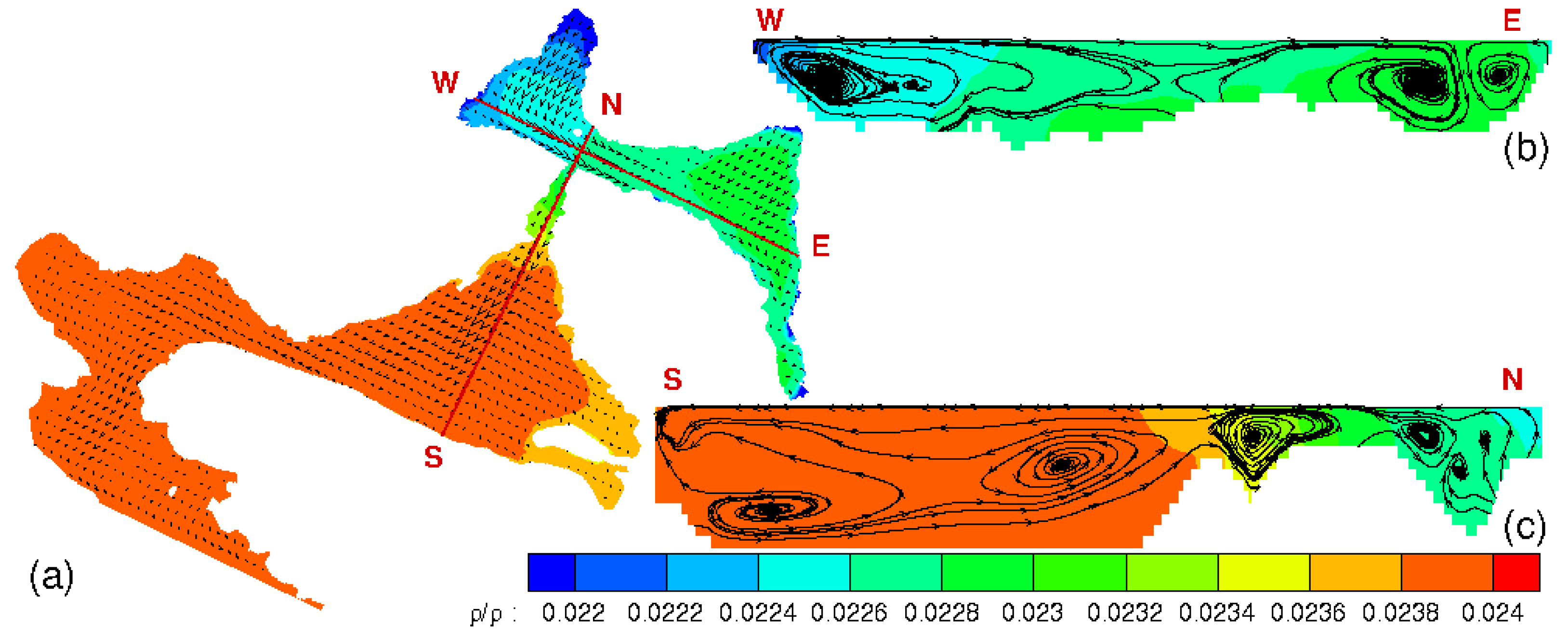
For the sea simulation, temperature and salinity fields are initialized according to literature field data of Boka Kotorska Bay [33,35], while, at the southwest boundary, Copernicus database values [36] are adopted. Density stratification is principally driven by temperature gradients in Kotor-Risan Bay. In the inner bay, the temperature varies from 24° (C) at the surface to 17° (C) at the bottom, while the salinity varies from 33 (PSU) close to the surface to 36 (PSU) at the bottom. In the other bays, the vertical distribution of the two quantities is almost constant with values approximately of $T=24$° (C) and $S=38$ (PSU).

Oil spill simulations are set considering a ship collision that releases a light oil (CPC-BLEND), with density ${\rho }_o$ = 809 kg/m${}^3$ and a pour point of −36° (C), low enough to prevent formation of tars. In Figure 2, the yellow line indicates the ship navigation route as reported in [10], obtained from [11]. The accidents are assumed to happen along the path in Verige Strait, the narrowest region of the bay. The red dots in Figure 2, labeled with letters (a)–(h), indicate the oil release points. The spill rate reproduces a tub emptying process, considering a total amount of spilled oil of V = 1400 m${}^3$, in 4 h.

3. Results

In this section, we show and describe the dynamics of low-atmosphere, sea and oil spill, first for the Bora wind scenario and successively for the Libeccio one. Finally, we analyze the effect of wind stress on oil slick dynamics.

3.1. Low-Atmosphere Simulations for Bora Wind Scenario

Figure 3 shows the wind velocity magnitude and vectors obtained from low-atmosphere simulations. Panel (a) shows the contour plot of wind velocity 10 m above the sea level in the LASc. The immersed bodies adopted to reproduce mountains surrounding the bay, are represented by green-brown contour plot. Panel (b) shows the inhomogeneous map of wind velocity obtained over the bay in simulation LASf; there are regions where the magnitude of horizontal velocity is close to zero, especially by the leeward side of the surrounding mountains. For example, in panel (c), a recirculation zone leeward a hill is well visible at a vertical cross-section over Herceg-Novi Bay. The position and direction of the section is marked by a red line and rectangle in Figure 3b.

3.2. Sea Current Simulation for the Bora Wind Scenario

Figure 4a shows the surface contour plot of the horizontal instantaneous velocity field. The horizontal space variability of wind stress directly affects the sea current, which flows from the inner bay towards Adriatic Sea. The red lines indicate the position of two vertical sections (W-E Figure 4b and N-S Figure 4c). The flow features within the fjord are made evident by streamlines: at the surface, the current follows the wind direction, while, at the bottom, it flows in the opposite direction. These up-welling and down-welling phenomena are typical in coastal regions. On the vertical section, horizontal axis vortices, spanning all over the water column, are visible. Such structures generated by wind stress at the sea surface have also been observed previously in [15,17].

Horizontal and vertical distributions of water density are shown in Figure 5. Panel (a) illustrates density variations at the surface layer; we notice that in the Kotor-Risan Bay, more than in other bays, sea currents are driven by both wind stress and density differences. Panels (b) and (c) show vertical distribution of density in two cross-sections indicated by red lines in panel (a). In Kotor-Risan Bay (panel (b)), analysis of the contour plot and streamlines suggest that wind stress is able to break stratification, thus enhancing water mixing along the vertical depth: lighter surface water is transported towards the denser region along the wind direction. This phenomenon appears more pronounced in panel (c), which shows that low-density water is pushed by wind from Kotor-Risan Bay towards Tivat Bay. The horizontal axis vortex developing in Verige Strait is promoted by both bathymetry and the horizontal stratification effect.

3.3. Oil Spill Simulation for Bora Wind Scenario

Figure 6 shows different oil spill scenarios, simulated for the Bora wind case. Following a typical ship’s path, from Kotor harbor to Kumbor Strait (yellow line in Figure 2), oil is released at different points (identified by panels from (a) to (h)) along the route. Film thickness contour lines of $h={10}^{-3}$ mm show the oil slick position at different simulation times after the initial release, $t_r$: $t_r=5$ min (red line), $t_r=1$ (green line), $t_r=5$ h (purple line) and $t_r=12$ h (blue line). Vectors indicate the direction and intensity of currents at the sea surface (dark gray), and wind velocity 10 m above sea level (orange); for clarity, vectors are shown every 20 grid cells in both horizontal directions and wind velocity vectors are scaled by a factor of 0.01. For each scenario, the area of interest for the oil spill event is shown on the left; on the right, we show a zoom over the oil slick, in order to better visualize oil spreading and transport dynamics.

In the first scenario (Figure 6a), oil is released in the narrow bay (700 m wide) close to Kotor harbor. Here, both sea currents and wind are weak and the slick spreading is driven by gravity force rather than friction. One hour after the spill, the slick reaches the eastern coastline, and, later on, the western one. Five hours after the spill, the slick spreads over the entire narrow strait and, after twelve hours, the oil slick occupies an area of about $6·10$${}^5$ m${}^2$, still moving towards Kotor harbor and slipping along the coastlines.

At the second release point, wind and sea currents are relevant (Figure 6b). During the first hour after the spill, oil starts spreading in the direction of the wind and is transported southward by the sea current towards Kotor harbor. Five hours after the spill, the slick reaches approximately the position described in the previous scenario. Here, wind and sea currents are weaker and the oil slick starts spreading radially driven by gravity force, similarly to the case of scenario (a).

In panel (c), the release spot is in the central part of Kotor Bay (Figure 6c), where wind and current point westward. Oil impacts on the southern coastline and is then transported by currents northward, close to Verige Strait, where sea currents flow in the direction opposite to the wind. Once oil reaches the northern coastline, it starts accumulating and then spreads driven by friction and gravity forces. The flow pattern of recirculation wind in this area makes the evolution of the oil slick more complex. Wind is weak because of the presence of mountains and the opposite sea currents (from Risan and from Kotor Bays, respectively) drive oil towards Verige Strait.

Panels (d) to (f) show the evolution of oil spill taking place in the Verige Strait. In each scenario, oil is transported mainly along wind and currents’ directions. In the scenario shown in Figure 6d, oil reaches the eastern shore of Verige Strait in less than one hour. Later on, because of lateral spreading, the slick also reaches the other side of the strait, covering a distance of about 150 m. Five hours after the spill, the slick occupies the whole strait area. After 12 h, the slick is transported inside Tivat Bay, where it finally reaches the southern coastline and starts accumulating because of the overall weaker transport velocity. In scenario (e), oil reaches the southern coastline about five hours after the spill and then it starts accumulating along the shore. Scenario (f) is similar to the aforementioned one; oil spot is 3 km south with respect to the previous scenario and the slick impacts the shore sooner.

In the scenario illustrated in Figure 6g, the oil slick spreads along wind and sea currents and it moves towards Kumbor Strait. Five hours after the spill, the oil slick reaches the southern shoreline where it starts accumulating and to be transported towards the strait along the coastline.

Finally, for the scenario with oil release spot in the Kumboir Strait (Figure 6h), where wind stress is weaker, the slick is spread mainly by friction and gravity force. The slick advection velocity is slower than in previous scenarios because of the lower wind friction in the area. In five hours, the slick impacts both shores of the strait and it moves towards Herget-Novi Bay.

3.4. Low-Atmosphere Simulations for Libeccio Wind Scenario

In Figure 7, we show wind horizontal velocity 10 m above the sea surface obtained in the two low-atmosphere simulations of Libeccio wind case. In panels (a) and (b), we show contour plot of wind velocity obtained in the LASc and LASf, respectively (note that the green-brown contour plot in panel (a) illustrates the immersed body used to reproduce the topography around the bay). For clarity, velocity vectors are plotted every 16 nodes in the horizontal directions. Similar to the Bora wind scenario, regions with different wind stress intensities can be identified. In Tivat Bay, at the entrance of Verige Strait, the wind accelerates and reaches a peak value of about $U_{10}$ = 10 m/s.

3.5. Sea Current Simulation for Libeccio Wind Scenario

Contour plots of the horizontal velocity and vectors in Figure 8a indicate the intensity and the direction of the surface current. It moves along the wind direction and become more intense in correspondence of wind peaks. In the vertical sections W-E (Figure 8b) and N–S (Figure 8c), the streamlines show the behavior of fluid flow along the vertical direction. At the surface, the current is aligned with wind direction and flows from Tivat Bay to the inner one, while, at the bottom, the current moves in the opposite direction. Close to the coastline or in correspondence of rapidly varying bathymetry, up-welling and down-welling phenomena are visible.

3.6. Oil Spill Simulation for Libeccio Wind Scenario

Figure 9 illustrates oil spills events for Libeccio wind case. In the following, all notation, colors, resolution and scaling factors are the same as for the Bora wind case, if not explicitly reported.

The oil spill dynamics, in all the distinct scenarios under Libeccio wind conditions, seem to indicate Kotor Bay as the most sensitive area in case of an oil spill accident. In fact, in all cases shown in Figure 9a–h, the oil slick is transported towards the northeast in Kotor Bay, where both wind and sea currents entrap the oil.

In the first scenario, shown in Figure 9a, oil starts spreading immediately after the spill under the action of gravity force rather than friction, since wind and sea currents are weak in this region, as also observed for Bora wind scenario. One hour after the spill, the slick impacts the western shore and from here it starts spreading northward along the coastline; then, it starts to be drifted eastward under the action of the more intense wind. Finally, it impacts the eastern coastline about twelve hours after the spill.

In the second scenario, panel (b), wind and currents are stronger at the oil spill location: the slick is immediately transported toward the eastern coastline. The impact takes place at about $t_r=1$ h. Then, the slick is driven northward along the shore and eventually gets trapped in the bay.

The oil spill scenario shown in Figure 9c is similar to the one described in (b): oil is firstly transported towards the eastern coastline in less than one hour, and then it moves along the coastline toward the bay.

In the scenario in Figure 9d, oil is released immediately after the Verige Strait. The slick impacts the portion of coastline situated in front of the strait, in less than one hour after the spill, and then it travels along the coastline towards the inlet.

In the scenario illustrated in Figure 9e, oil is released at the entrance of Verige Strait. In less than one hour, the slick impacts the eastern coastline of the strait first, and, later on, the coastline in front of the mouth of the strait. From here, oil is further transported along the coastline. Inside the strait, a fraction of the oil slick slows down and starts accumulating on the strait shore, slowly releasing more oil in the bay.

In scenario (f) (Figure 9f), the oil slick moves towards the Verige Strait and impacts its eastern shoreline in less than one hour. At about $t_r=5$ h, it reaches the coastline in front of the strait and then it slips along the shore eastward. As in scenario (e), a part of the slick slows down, impacting the shore, releasing an elongated tail, departing from the main slick.

In scenario (g) (Figure 9g), oil spreads along the wind direction towards the Verige Strait. In about one hour, it impacts the western coastline at the entrance of the strait, and then it is transported by wind and currents on the other side of the strait. As for scenarios (e) and (f), when part of the slick starts slowing down approaching the shore, an elongated tail departs from the main slick. At $t_r=12$ h, part of the oil is still located along the eastern strait’s shore.

The last scenario is illustrated in Figure 9h. The spill occurs in an area where both wind and sea currents are weak; therefore, as mentioned in scenario (a), oil spreads radially mainly due to gravity force. A part of the slick reaches the southwestern coastline where wind and sea currents are almost absent; here, oil starts to accumulate along the shore. Another part of the slick meets stronger currents and starts to spread along the flow direction. At the $t_r=1$ h, the slick has also reached the northwestern coastline. The slick is then transported through Tivat Bay along the coastline, and, in the meantime, part of the oil from the slick accumulated along the southwestern shore starts detaching. As a consequence of this continuous release of oil along the coastline, the oil slick is much larger than in the other scenarios analyzed. Five hours after the spill, the oil slick arrives at the entrance of the Verige Strait. Twelve hours after the spill, the slick crosses the Tivat Bay and Verige Strait. Part of the oil is accumulated at the entrance along the western coast and at the eastern shore of the strait. The slick also reaches the coastline in front of the straits and it is transported eastward.

3.7. Effect of Wind Stress Parametrization on Oil Slick Transport

In most models present in literature, oil slick advection velocity is given by the sum of two contributions proportional to sea current and wind velocity, respectively (see Equation (9)). Usually, for sea current, the drift coefficient is set equal to $1.0$, while the wind drift factor adopted is $k_w=0.03$ [8,9,28]. More recently, some authors proposed different values for the parametrization, as, for example [2]. They calibrated the drift coefficients of their oil spill Lagrangian model using trajectories of buoys; the wind drift coefficient was found to be $k_w=0.005$, a value one order of magnitude smaller than the standard literature one. Such difference can completely modify the trajectory of the spill predicted by the model. At the moment, we cannot draw any conclusion on the correct value to be used in simulations, especially in the presence of Eulerian models. However, assessing the difference in results considering the two values can shed light upon the necessity of more fundamental work on the topic. For this reason, we apply the newly proposed parametrization value in the scenarios studied in Section 3.3, for the Bora wind case, considering the release points (d) and (e). In such cases, the relative importance of wind and sea current can lead to completely different predicted trajectories. Both points are located in Verige Strait, which is surrounded by mountains rising up to 600 m. In this canyon, the wind blows from Kotor-Risan Bay towards Tivat Bay. With the standard $k_w$ value, the slick spreads along the wind direction while lateral diffusion is inhibited. The wind stress is dominating over the other forces. The oil slick moves following the path where wind and currents reach the maximum velocity as can be deduced by an analysis of the wind and current. Figure 10 shows a vertical cross-section downwind the Verige Strait, the position being indicated by the red line in the black top view of the bay. Contour plots indicate the plane-normal velocities for air and water flows, in the upper and lower panels of the figure, respectively. The dark green line indicates the position and the extension of the oil slick at $t_r=12$ h, for scenario (d). We can notice that, leeward, the Verige Strait, the velocity of wind and sea current are higher and move from the strait towards the bay; oil slick is located in the area where both wind and sea currents are stronger.

On the other hand, the use of $k_w=0.005$ produces a variation of the trajectories as depicted in Figure 11 for scenarios (d) and (e). In scenario (d), oil is transported slower and it spreads laterally and backward in the Kotor Bay. At $t_r=12$ h, the oil slick has moved along the wind direction inside the strait, but also against wind, following the sea current close to the southern coast of the Kotor Bay.

In scenario (e), the slick spreads laterally following the sea current. After $t_r=12$ h, the slick is still in the middle of the bay.

This brief analysis highlights the importance of a correct wind stress parametrization in order to correctly predict oil slick trajectory and spreading, especially in the presence of complex air and sea flows as in coastal areas. The new parametrization seems to have a minor impact in case of a strong wind, while, in case of light wind, it overestimates the effects of sea currents in oil slick transport, as we can observe in Figure 11, for the scenarios (e) (on the right panel) and (d) (on the left panel), respectively.

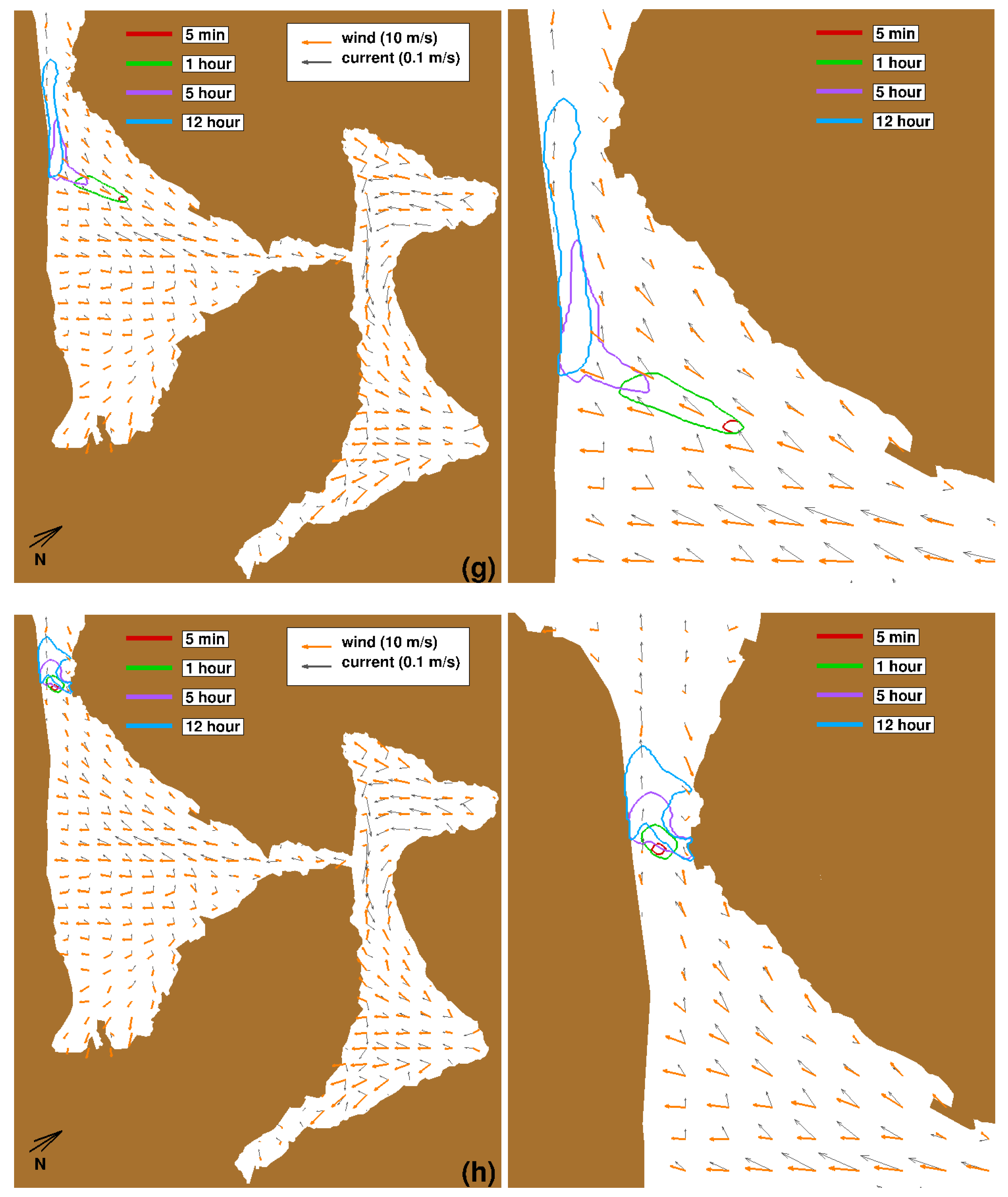
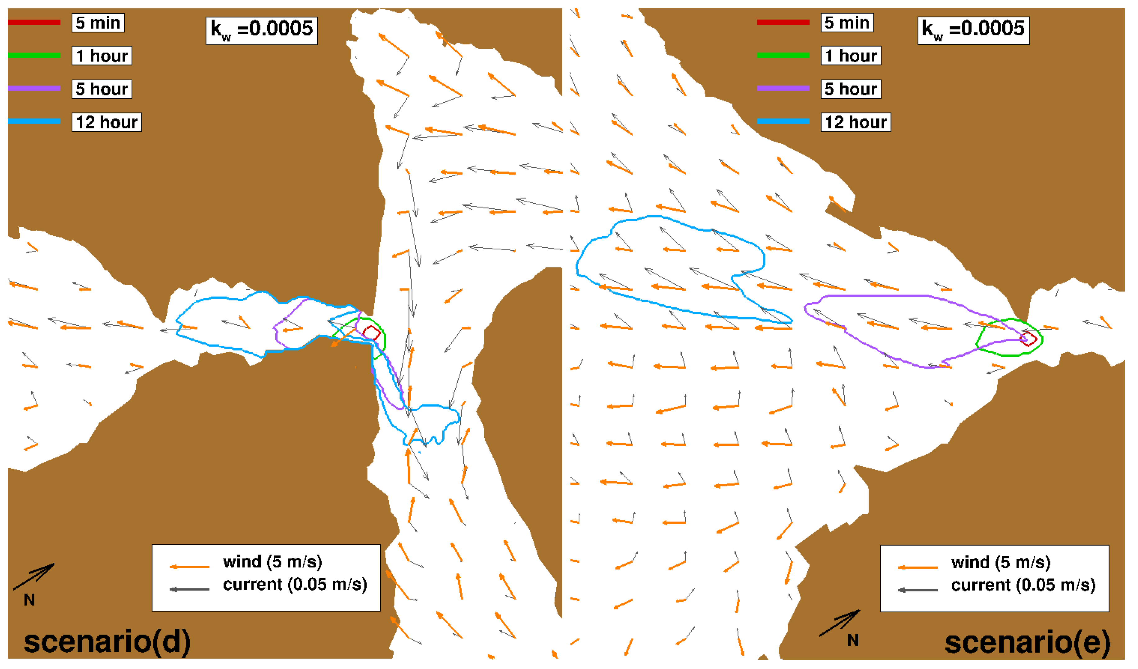
4. Discussion

In this study, we analyze the dynamics of a hypothetical oil spill accident in the Boka Kotorska Bay, a fjord characterized by a rapidly varying orography, a complex bathymetry and sinuous coastline. A high resolution model is used to reproduce this complex dynamics and to obtain reliable oil slick predictions. In this study, the oil model does not take into account the weathering processes, in order to underline the role played by wind and sea current on the oil fate. Its inclusion will be considered in future works.

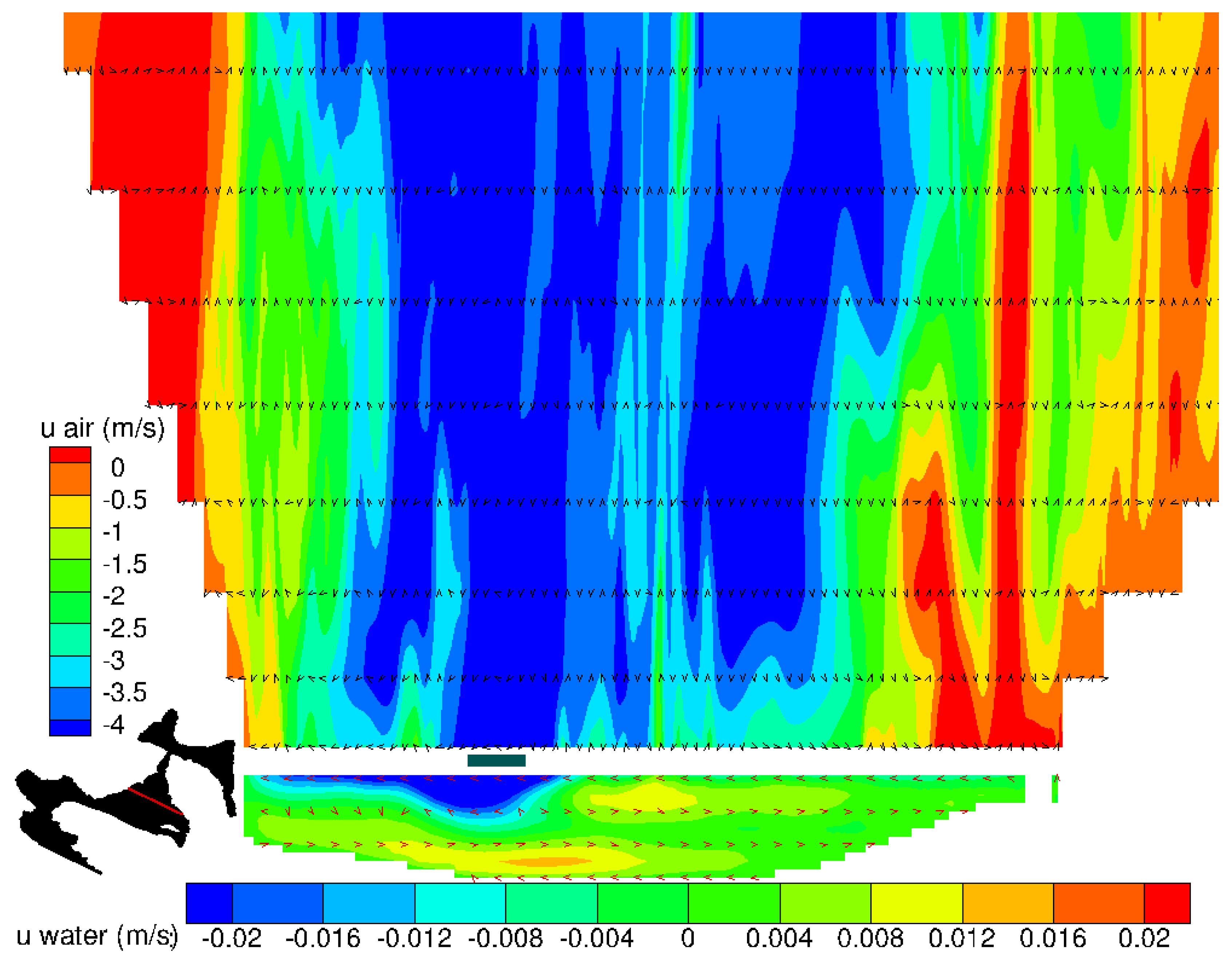
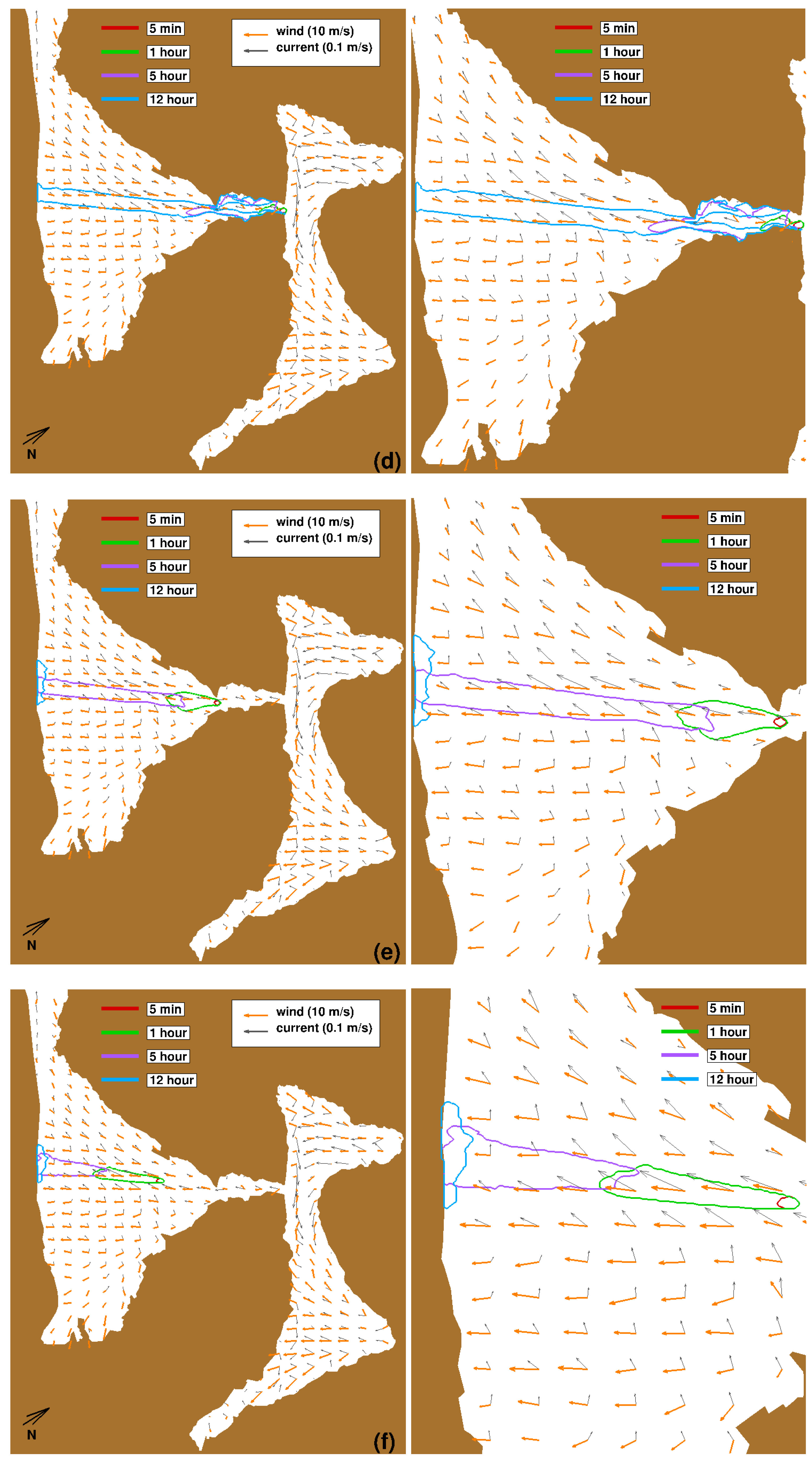
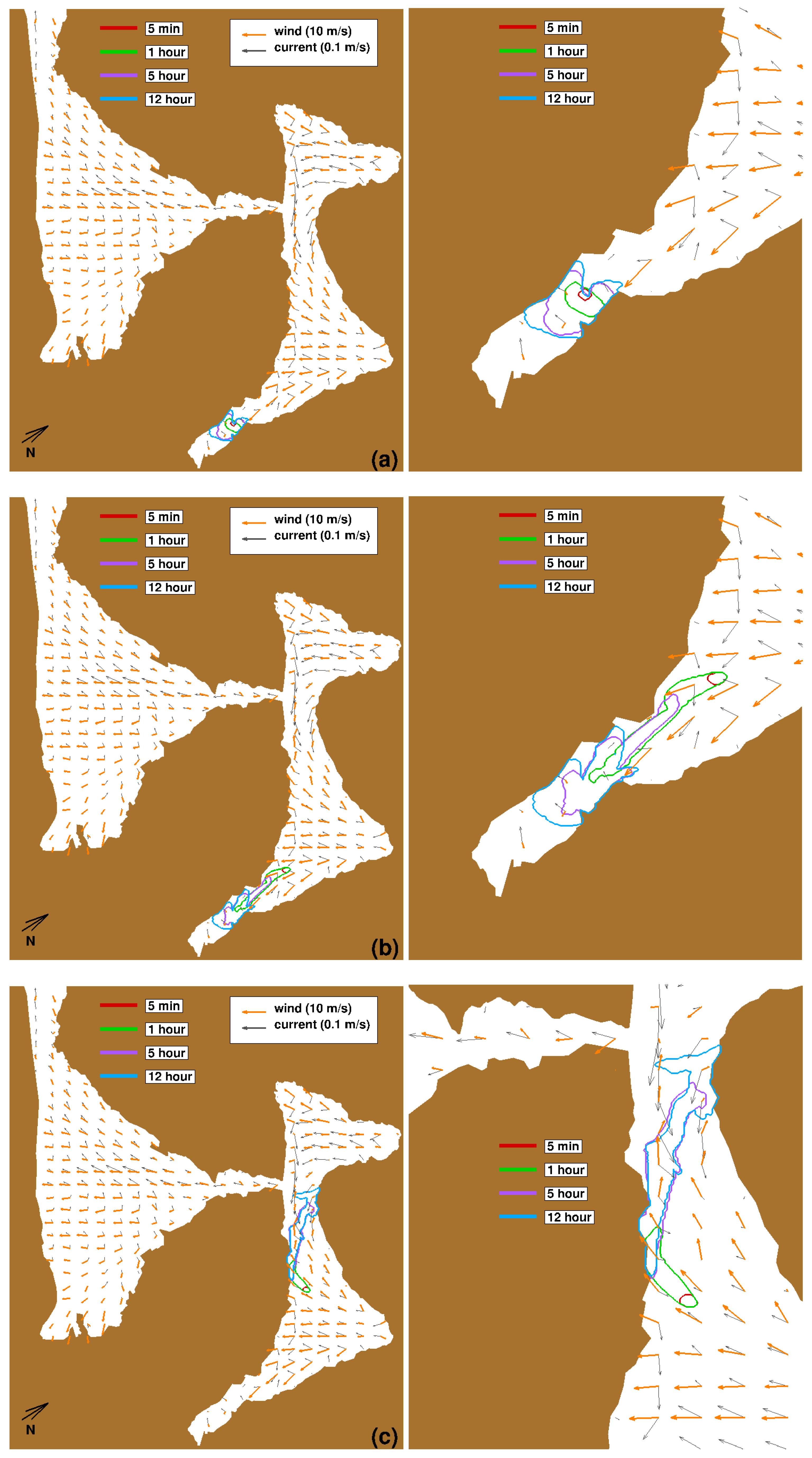
As suggested in [17], the complex orography can affect the horizontal distribution of wind stress in the bay, making it highly inhomogeneous. For this reason, two low-atmosphere simulations are run: LASc uses a large domain with a coarse grid, LASf uses a small domain with a fine grid. The latter provides an accurate distribution of the wind stress, used for both marine and oil simulations. The analysis of low-atmosphere results highlights the presence of zones where wind stress is strong, spots where wind is almost absent or even recirculating in the opposite direction. The wind stress is adopted as surface boundary conditions for marine simulations. We investigate different oil spill scenarios, characterized by different locations of oil release within the bay, along the ship route. We consider two meteorological conditions: Bora wind (NE), which is the most frequent wind in the area; Libeccio wind (SW). We consider a summer situation, in which river runoff is almost absent and river discharge in the bay can be neglected. The absence of river runoff and hence lower outflowing currents turn out to be pejorative since the pollutant remains longer in the bay.

In both cases, we find that oil slick approaches the coastline in few hours and then it spreads along it, constrained by wind forcing and by the alongshore surface sea current. This small time scale underlines the need of contingency plan for this type of situation, allowing for an effective pollutant mitigation action.

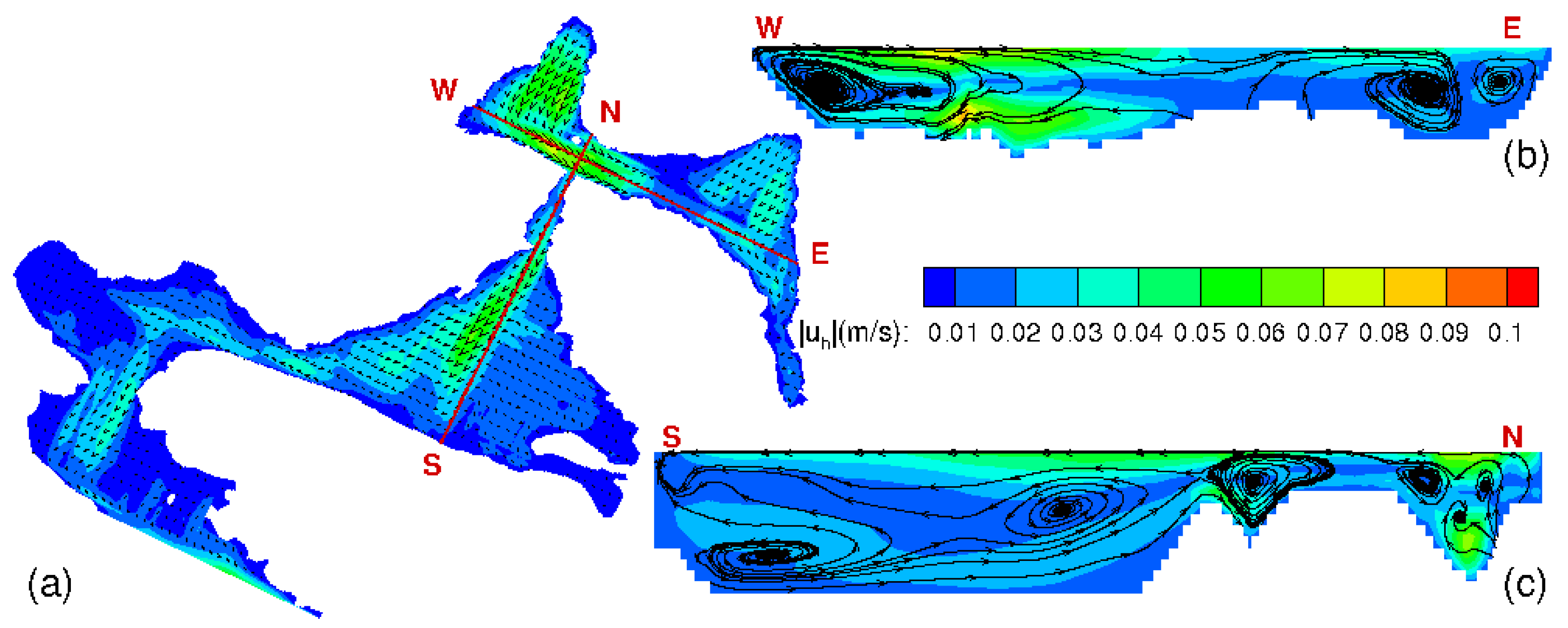
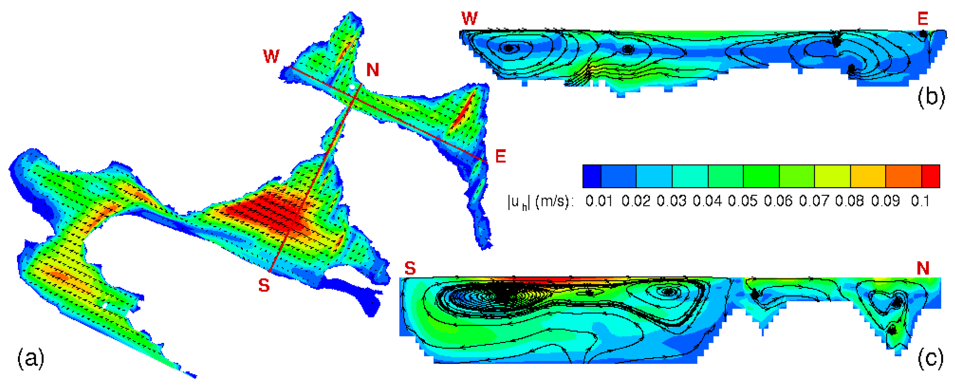
The complex orography has a strong impact on the oil slick because wind flow is influenced by the presence of the mountains. This aspect and its interaction with the coastline generate complex flow patterns at the sea surface, eventually influencing pollutant dispersion.

On leeward coastline, because of the mountains, the wind exhibits separation, with low stress regions and recirculations with respect to the wind direction. On the windward coastline, down-welling takes place, but, due to the mountains on the same side, the wind is then forced to blow parallel to the coastline, and the sea current adjusts accordingly. This behaviour is accentuated under strongly stratified water column, since the energy transfer from the wind to the sea, is confined in the upper water layer; this results in an intensification of the horizontal component of the surface current, rather than in an increase of down-welling.

Depending on the wind direction, the gulch between Tivat Bay and Risan-Kotor Bay behaves as a bottleneck (see Libeccio case), where the wind, constrained by converging mountains, accelerates increasing the stress at the sea surface. Moreover, the wind, constrained by lateral and bottom boundaries in the fjord, forms secondary flows characterized by vortexes elongated in the streamwise direction. The resulting stress at the sea surface reduces lateral oil spreading.

The complex orography and coastline also determine areas where the sea current is opposite to the wind direction. Considering Bora case, scenario (c), such effect is evident and could trigger counterintuitive oil spreading: sea current flows in one direction while the oil spreads on the opposite one. In this kind of analysis, the wind parametrization adopted in the oil model becomes crucial for cases where air and surface water move in opposite directions. As underlined by the numerical simulations, variations in the wind parametrization can bring to completely different spreading scenarios. In this study, we adopted the literature’s widely accepted value and successively, for two spill scenarios, we re-run some cases with a smaller value recently proposed in literature. The differences are significant.

These aspects show the difficulties in the prediction of oil fate in such a complex situation, and that a proper wind pattern representation, together with a robust wind stress parametrization for the oil model, are of crucial importance.

References