Article

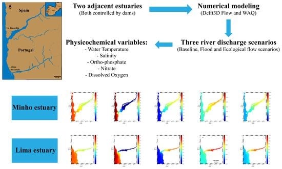
Modeling the Impact of Extreme River Discharge on the Nutrient Dynamics and Dissolved Oxygen in Two Adjacent Estuaries (Portugal)

1
CESAM-Centre for Environmental and Marine Studies, Physics Department, University of Aveiro, Campus de Santiago, 3810-193 Aveiro, Portugal
2
CESAM-Centre for Environmental and Marine Studies, Biology Department, University of Aveiro, Campus de Santiago, 3810-193 Aveiro, Portugal
*
Author to whom correspondence should be addressed.
J. Mar. Sci. Eng. 2019, 7(11), 412; https://doi.org/10.3390/jmse7110412
Submission received: 18 October 2019 / Revised: 7 November 2019 / Accepted: 11 November 2019 / Published: 13 November 2019

Abstract

:
The Minho and Lima are adjacent estuaries located in the north of Portugal, with high ecological and economic importance. To address gaps in knowledge about changes in nutrient patterns in adjacent estuaries subject to different freshwater inflows, a numerical model, Delft3D, was implemented and developed, using a single domain, which allowed physical communication between estuaries. Calibration and validation of the model was successfully performed. Three numerical simulations were carried out, in which only river flows were varied (1st corresponds to a baseline numerical run, the 2nd a flood scenario, and the 3rd a drought scenario). Under flooding conditions, similar patterns were verified in both estuaries, with high fluvial discharges showing to have a reduced impact on both estuarine dynamics. In this case the nutrients were not a limiting factor for the biota, both for summer and winter seasons, since there was no significant decrease in dissolved oxygen concentration. For the drought scenario, it was observed that the estuary with the lower inflow of freshwater (Lima) was the most affected, with a significant decrease in the concentration of nutrients and oxygen dissolved in the winter season (decrease of 2 mg O2/L). In conclusion, this work reveals that it is essential to continuously monitor dam-controlled estuarine systems, as a significant decrease in river discharge will cause significant changes in the variables analysed (O2, PO4, and NO3) and may cause loss of biodiversity.

Graphical Abstract

1. Introduction

Estuarine systems are highly dynamic since their geomorphology (processes of erosion and sedimentation) and their physicochemical properties are constantly changing [1]. These physicochemical changes are strongly influenced by atmospheric and hydrodynamic processes (waves, tides, wind stress, freshwater discharges by rivers, and exchanges with the atmosphere) making the estuaries very productive systems that play a very important role in biogeochemical cycles, intercepting watershed-derived materials before delivering them to the marine environment [2], and influencing the sedimentation rate, zonation and species productivity, water temperature, and salinity of each zone [3]. These very complex features of estuaries enable them to have a high primary production, due to nutrient fluxes from both rivers and coastal upwellings, which is very valuable since they have high metabolic rates and serve as important sites for water filtration and nutrient retention, transformation, and recycling [3,4,5,6]. For this reason, there is particular interest in these ecosystems, both ecologically and economically.
In the last 50 years, human activity and climate change have greatly transformed estuaries, of which some transformations have already been documented [7,8,9,10,11]. One of the current main concerns about estuaries is climate change and the resulting impact of extreme events on water quality [12,13,14]. Since river flow is a useful indicator of freshwater availability, it can be used to indicate likely impacts of climate change on water resources [15]. In estuarine areas, one of the main impacts of climate change is the variation in river flow, which induces frequent flood or drought events with higher intensities [16]. Furthermore, because of water circulation and oceanic volume changes, estuarine and coastal systems are predicted to experience a loss of marsh and intertidal habitats, a greater marine intrusion or freshwater plumes, and increased eutrophication, hypoxia, and anoxia [17,18,19]. Additionally, an increase in water temperature, a decrease in mean precipitation, and a higher frequency of extreme weather events are expected, with short episodes of intense precipitation, drought periods, and heat waves, which will make estuaries even more vulnerable. Recently, more frequent occurrences of intense flood events and tropical cyclones are likely to generate large infrastructural damages as a result of flooding, high winds, and higher storm surges [20], but they can also lead to prolonged large-scale stratification in estuaries and coastal regions as a result of large freshwater influxes [21,22]. The stronger stratification and elevated nutrient and organic matter loading to estuarine and coastal systems, associated with these extreme climatic events, along with the increase in temperature already observed in some coastal ecosystems [23,24] could lead to the development of bottom water hypoxia [20,22,25]. It is well-known that oxygen solubility decreases with increased water temperature and salinity, while decomposition of organic matter by bacteria will consume oxygen [26,27]. In addition to these aspects, other factors contribute to the alteration of estuarine dynamics and to the degradation of water quality, such as the construction of upstream river dams and the existence of punctual and diffuse discharges along the estuaries that release high concentrations of nutrients and contaminants, of which this movement may be also altered by climate change through increased atmospheric deposition and surface run-off [28,29,30]. Studies on the impact of dams on estuaries have been carried out around the world to try to understand their effects on various physicochemical variables [31,32,33,34]. Despite this framework, there is little evidence-based research on the effects of climate change drivers on estuarine dynamics, except for the effects of temperature and sea-level rise [35,36,37]. To explain the existing and predictable biogeochemical processes in estuaries, numerical models are used nowadays since they show many important advantages [38,39,40,41], and they can serve as predictive or decision support tools [42].
The estuaries researched in this study (Minho and Lima) are located adjacent to each other (Figure 1A), at similar latitudes, and are subject to the same atmospheric, environmental, and oceanic conditions, but under completely different fluvial freshwater inputs (Minho River base flow is higher than Lima base flow). By these reasons, they constitute ideal systems to assess how changes in freshwater inflows induced by climate change will impact estuarine nutrient dynamics and dissolved oxygen.
In addition to the aforementioned, the hydrographic region of Minho and Lima (northern Portugal) is highly attractive, supporting important urban uses (e.g., generation of electricity from dams) and economic activities such as port activities, industrial navigation, fishing and tourism, recreation, and leisure. Besides being important at the economic level, these estuaries present marine prairies (e.g., seagrass) that function as natural nurseries for numerous species of great economic importance, particularly invertebrates and fish. In ecological terms, these systems function as biological filters of nutrients and pollutants, and they play a key role in controlling coastal erosion and carbon sequestration. According to “Plano de Gestão da Região Hidrográfica do Minho e Lima” (PGRH1) [43], the hydrographic region of Minho and Lima (northern Portugal) has a high ecological value since it has a great diversity of habitats, including marshes, reeds, and sandbanks, and, in addition, it presents two Protected Areas for Birds, six Sites of Community Importance, and four Protected Areas [43]; thus, these two estuaries confer important protection statutes such as the Rede Natura 2000, Special Protection Area for Birds (SPA), Important Bird Area (IBA), and Biotope CORINE. For these reasons, because of its strategic location, there is particular interest in these ecosystems, both ecologically (e.g., they host a great wealth of organisms, a wide diversity, and are also highly productive) and economically (e.g., aquaculture, sheltered areas for the construction of ports and leisure areas). These characteristics translate into enormous socio-economic benefits for the surrounding fishing populations, who traditionally live off the harvesting of shellfish and fishing.
In this way, because of the importance of these two estuaries, the present work intends to study the possible impacts of climate change on water quality of the adjacent estuaries under study through the application of a numerical model, Delft3D, focusing on the occurrence of extreme river discharge events. Specifically, the impacts on nutrient dynamics and dissolved oxygen will be assessed as well as the potential impacts on estuarine ecological quality, health, and economic resource utilization. The assessment will be in compliance with EU Directives in order to provide a baseline within which the magnitude of change from current activities or events can be evaluated and remediation can be planned.

2. Materials and Methods

This section describes the study area; the in situ data; the procedures followed in the model implementation, including calibration and validation; as well as the definition of the scenarios proposed to achieve the objectives of this work.

2.1. Study Area

The Minho and Lima estuaries (Figure 1B,C) are located on the northwestern Portuguese coast, between the coordinates 41°36′N and 42°2′N latitude and between 8°24′W and 8°54′W longitude.
The Minho River (Figure 1A) begins in Spain (Serra de Meira) and flows into the Atlantic Ocean between La Guardia (Spain) and Caminha (Portugal). This river serves as a northern border between Portugal and Spain and has an approximate length of 300 km, of which 230 km is in Spanish territory and the remaining 70 km crosses into Portugal [44]. The main Portuguese tributaries are Trancoso, Mouro, Gadanha, and Coura rivers, while the main Spanish tributaries are Támoga, Ladra, Ferreira, Avia, Tea, Louro, Neira, Sil, and Arnoya rivers [45]. The Minho river presents an average annual discharge of 305 m3/s, and the monthly average discharge varies between 121 m3/s during the summer and 692 m3/s in the winter [39], which depends heavily on the discharges made by the hydroelectric dams that exist throughout its extension. The Minho estuary, during periods of high river flow, tends to have a salt wedge type [46]. It presents an average depth of 2.6 m [47], and the astronomical tide varies between 2 m during neap tides and almost 4 m in spring tides [46]. This estuary is considered one of the least contaminated along the Portuguese coast [48,49]; however, in Spanish territory, there is sporadic industrial pollution, mainly due to the industries in Porriño (Tui city) [50], that has been associated with the main cause of contamination of the Louro estuaries [50,51]. Beyond this source, the hydrographic basin receives diffuse pollution related to agriculture and the use of fertilizers [44].
The Lima River (Figure 1A) begins in Spain (Sierra S. Mamede) and flows into Viana do Castelo (Portugal). The Lima river is about 108 km length, of which 41 km is in Spanish territory and the remaining 67 km crosses into Portugal [44]. The Vez and Castro Laboreiro rivers are the main Portuguese tributaries. This river has an average discharge of 30 m3/s in the summer and 130 m3/s in the winter season [52], depending heavily on the discharges made by the dams in the region (Touvedo and Alto Lindoso). The Lima estuary has an average depth of 3 m, while a maximum depth of 8 m is observed in the navigation channels [53]. This estuary has a semi-diurnal and mesotidal regime (the high tidal range is 3.7 m and the low tidal range is 1.1 m) [53]. A general evaluation of the surface water quality reveals that the Lima river does not present significant levels of pollution that would prevent most of its use; however, there are some sections with strong bacteriological contamination [54], and polycyclic aromatic hydrocarbons (PAHs) and heavy metals are present in sediments [55]. These pollutants can come from the harbour of Viana do Castelo and from discharges of urban origin that are released without prior treatment by some municipalities [56].

2.2. In Situ Data Collection

The collection of in situ data is very essential to perform model implementation, calibration and validation, since this data will determine the degree of model reliability and accuracy.
Harmonic tidal constituent data for the Minho estuary were collected by Zacarias [57] between 20 February and 19 March 2006, while for the Lima estuary, these data were taken from the Portuguese Hydrographic Institute at the Viana do Castelo station. The six locations where the tidal surveys were carried out are represented in Figure 2A.
Regarding the water temperature, salinity, ammonia, nitrate, ortho-phosphate, and dissolved oxygen data, these were collected by Vieira et al. [58] during the period between February 2012 and February 2013. These measurements were collected one day a month along the Minho and Lima estuaries. To make these collections in the same location and at the same depth, Vieira et al. [58] defined seven transepts in each estuary (Figure 1B,C), in which they measured the coordinates of the sampling sites, as well as the depth of the site, using a GPS (HP IPAQ GPSMAP) and a depth gauge (Hondex PS-7). In each transept, a water sample was collected, and in situ measurements were made (water temperature, salinity, and dissolved oxygen) with a multi-parameter probe (VWR SP90M5) in 3 regions (south margin of the river, middle of the river, and north margin of the river). In each region, three replicates were made to obtain a better representation of the study area and to minimize errors. The water samples were collected with polyethylene–terephthalate bottles and stored at −20 °C for nutrient analysis [58]. The nutrient concentrations (ammonium, nitrate, and orthophosphate) were determined using commercial photometer kits (Photometer 7000, Palintest, Kingsway, England).
For the model validation, two sets of data were used. The first consisted of water temperature, salinity, and dissolved oxygen collected in 2013 (5 May to 5 July 2013) and extracted from a MeteoGalicia oceanographic buoy identified in Figure 1A (point P, “Boia de A Guarda”) (www.mandeo.meteogalicia.es). The second set of data was collected on 15 April 2019 in the transects of the Lima estuary represented in Figure 1C, which consisted of water temperature and salinity sampling.

2.3. Model Implementation

To study the impact of extreme river discharge events on the nutrient dynamics, the Delft3D model (www.oss.deltares.nl) was used. The period in which the simulations were carried out was from 1 January 2012 to 1 March 2013. In this work, the Delft3D-FLOW hydrodynamic module [59,60] and the water quality module Delft3D-WAQ [61] were applied. The hydrodynamic module, Delft3D-FLOW, allows working in 2 or 3 dimensions, and it solves shallow water equations based on Navier–Stokes three-dimensional and continuity equations using the finite difference method. In addition, the model simulates transport phenomena resulting from tidal and/or meteorological forcing, including the effect of density differences due to a non-uniform water temperature and salinity distribution (density-driven flow) [62]. The water quality module, Delft3D-WAQ, also allows working in 2 or 3 dimensions, depending on the choice made in the Delft3D-FLOW module. It solves the advection/diffusion/reaction equation on a predefined computational grid and for a wide range of model substances. This module allows to model a wide range of substances as well as processes. As Delft3D-WAQ is not a hydrodynamic model, it will seek hydrodynamic information from the Delft3D-FLOW module through a coupling process. This will extract velocities, water elevations, density, salinity, water temperature, vertical eddy viscosity, and vertical eddy diffusivity from the final Delft3D-FLOW simulation file [63].
Both modules were setup with an 835 × 170 cell curvilinear irregular grid with a mean resolution of ~50 m in the Minho estuary, ~30 m in the Lima estuary, and ~850 m at the offshore open boundary (Figure 2B). A single domain for the two estuaries allowed interaction between them, and a more realistic result is expected. Bathymetry used results from the interpolation to the numerical grid of a set of topohydrographic surveys. To force the Delft3D-FLOW module, the tidal harmonic constituents (to reproduce the tide), water temperature, and salinity data were used in the open boundary conditions, while wind and heat flux data were imposed in the ocean–atmosphere interface, and river discharges and water temperature were imposed in the river boundaries. The tidal data were obtained from TOPEX/Poseidon (www.jpl.nasa.gov) [64]. TOPEX/Poseidon is based on a global oceanic tide model (model NAO.99b), which provides the 13 tidal solution main constituents (M2, S2, N2, K2, K1, O1, P1, Q1, Mf, Mm, M4, MS4, and MN4) with a spatial resolution of 0.25°. Regarding the values of water temperature and salinity used in oceanic boundaries, the Copernicus Marine Environment Monitoring Service database was used (CMEMS, www.marine.copernicus.eu). The daily series of freshwater discharges and water temperature for the Minho and Lima rivers were obtained from the Confederacion Hidrográfica del Miño-Sil (www.chminosil.es) and the Sistema Nacional de Informação de Recursos Hídricos (SNIRH, www.snirh.apambiente.pt), respectively. For the Minho River, data were obtained from the Salvaterra do Minho station (N015), while for the Lima River, data were obtained from the Touvedo dam (03G/01A) automatic data network (turbinated flow data). To force the atmospheric boundary, daily atmospheric (relative humidity, air temperature, and net radiation) data from the European Center for Medium-Range Weather Forecasts (ECMWF, www.ecmwf.int) were used. Concerning the atmospheric pressure and the wind data (u and v components near the surface), these were retrieved from the Thredds Server of MeteoGalicia (www.mandeo.meteogalicia.es). To force the Delft3D-WAQ module, ammonia, nitrate, ortho-phosphate, dissolved oxygen, phytoplankton, and total net primary production data were used in the open boundary condition. Ammonia, nitrate, ortho-phosphate, and dissolved oxygen data were imposed in the river boundaries. The values of orthophosphate, ammonia, nitrate, dissolved oxygen, phytoplankton, and total net primary production imposed at the ocean interface were withdrawn from the CMEMS, and the biochemical data for the river discharges into the estuaries under study were taken from the HypeWeb model (www.hypeweb.smhi.se) because of the scarcity of observational data.
Since Delft3D-WAQ presents many processes and substances to be modeled, several numerical simulations were made aiming to select the most relevant processes and substances in estuaries under study and to verify if the model approached reality, by comparing model predictions with observed data, at the end of each new simulation. Given this, the most accurate numerical simulation processes and substances are presented in Table 1.

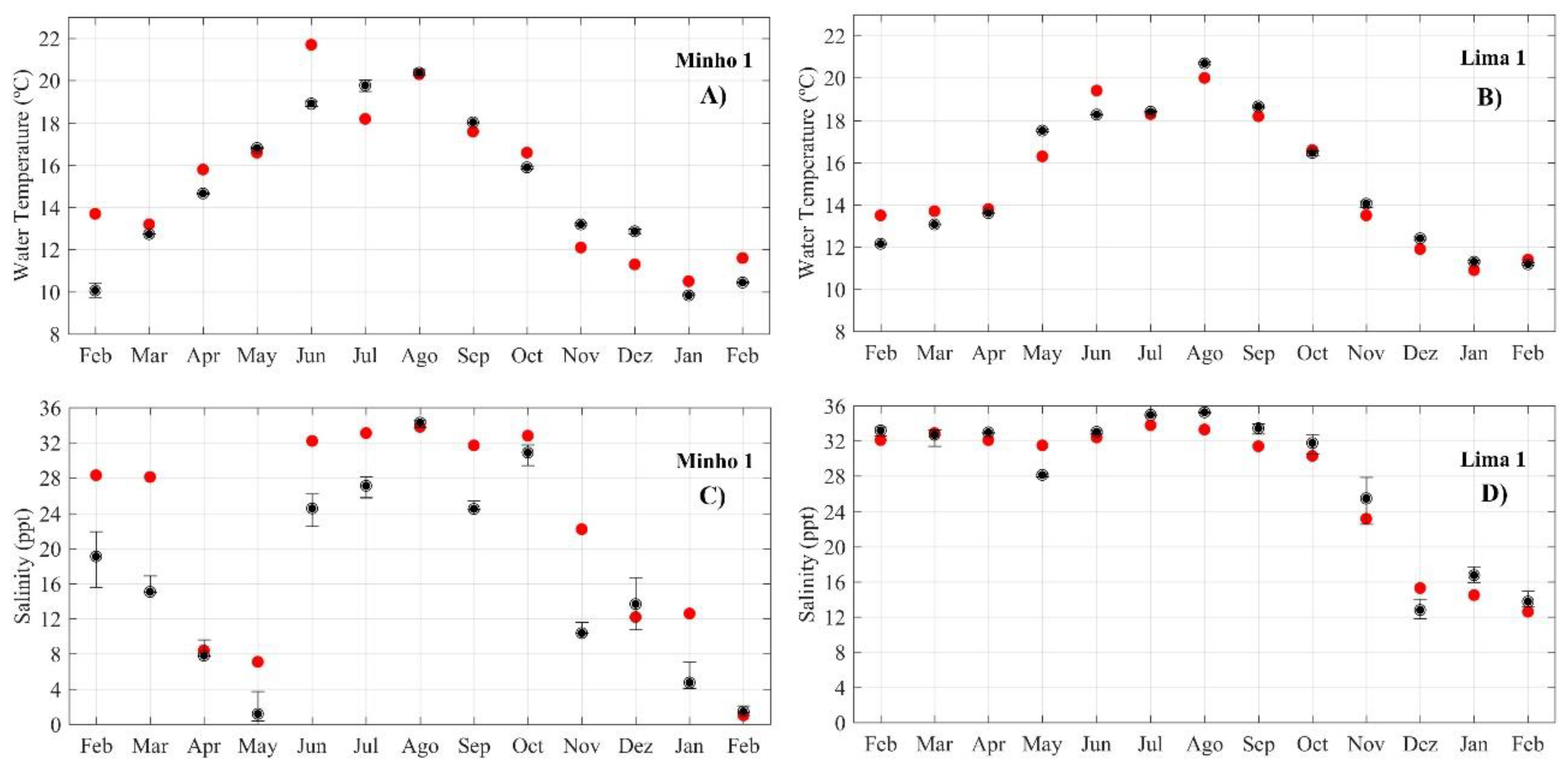
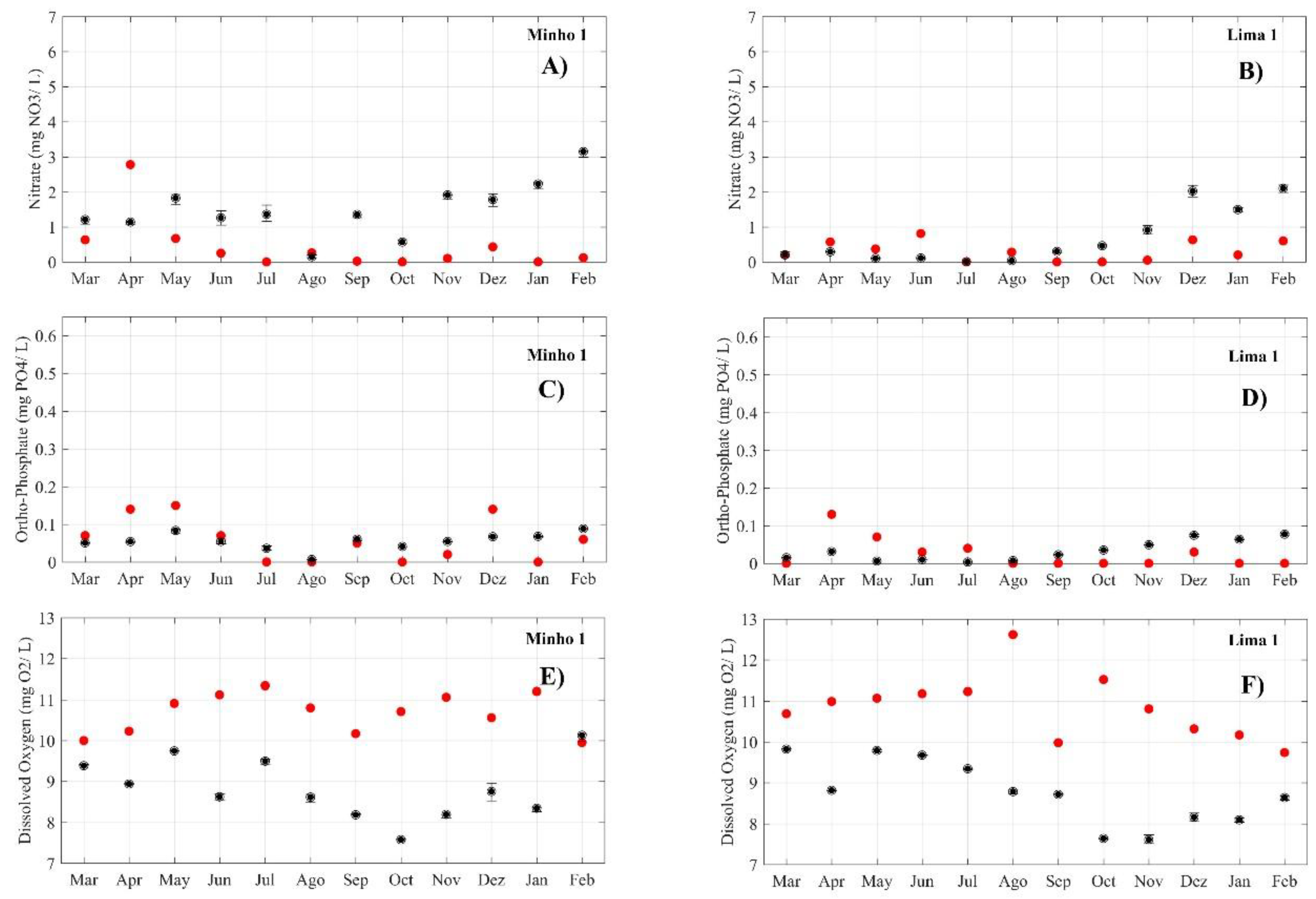
2.4. Model Calibration and Validation

Numerical model calibration and validation processes are important steps when performing estuarine modeling studies. Given the complexity of these models and the frequent data limitations (e.g., lack of continuous in situ data), it is rare to find studies performing both processes simultaneously, as recognized by Whitehead et al. [65] and Tomic et al. [66]. By these reasons, a large number of modeling studies perform only one of these processes (e.g., [67,68,69,70]), or alternatively perform both processes for a very limited period or even solely based on seasonal data ([71,72,73,74,75,76,77,78]). For the present study, and despite the common data limitations, both processes were performed for the hydrodynamic and water quality module in the Delft3D model implementation, following the procedures described below, and data sets presented in Section 2.2.
To calibrate the Delft3D-FLOW and Delft3D-WAQ modules, in situ data of tidal harmonic constituents, water temperature, salinity, ammonia, nitrate, orthophosphate, and dissolved oxygen were used. Model predictions for both estuaries were compared with in situ data following the procedures described by Dias and Lopes [79] and Dias et al. [80], and model accuracy was quantified for each numerical simulation performed. This quantification was performed using the root-mean-square error (RMSE) [81] and cost function (CF) [82]. To improve the fit between predictions and observations, the background friction and the total respiration flux were varied [83] for hydrodynamic and water quality modules, respectively.
In order to validate the hydrodynamic and water quality modules, water temperature, salinity, and dissolved oxygen model predictions were compared with independent in situ data. The adjustment between predictions and observations was quantified through RMSE and CF computation.

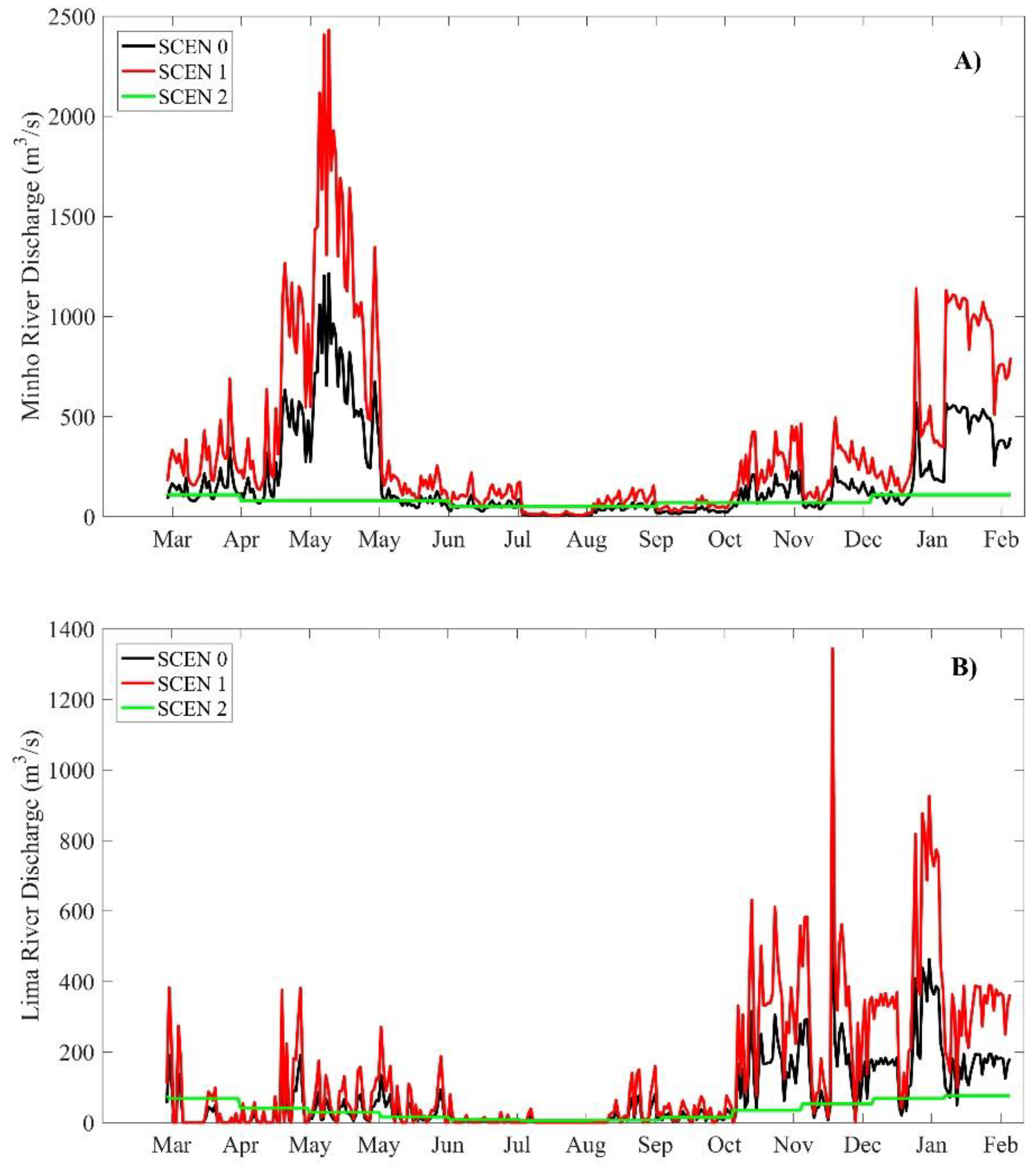
2.5. Model Scenarios

Considering the predictable climate change impacts on river discharges, with an increase in the frequency and intensity of extreme events [84], three different scenarios were designed to investigate the impact of extreme inflow conditions during one year (1 March 2012 to 1 March 2013) in the studied system of coupled estuaries (Figure 3A,B). The only factor that changed between these scenarios was the Minho and Lima river discharge, keeping the remaining inputs of the model unchanged. The first simulation corresponds to the case of numerical simulation used for model calibration, serving as baseline (hereinafter referred as SCEN 0), and the remaining two correspond to a flood scenario (SCEN 1) and a drought scenario (SCEN 2) (Figure 3A,B). In SCEN 1, river discharges were considered to have twice the discharge as that of the calibration simulation (SCEN 0). This relation was based on a comparison between data used in SCEN 0 and the historical fluvial discharge obtained from HypeWeb model (www.hypeweb.smhi.se). In SCEN 2, only the ecological discharges (minimum flows released by dams in the event of drought) were considered. Ecological flow data at the river boundary was based on reports from the Região Hidrográfica do Minho e Lima of the Agência Portuguesa do Ambiente [85] and in the Boletín Oficial Del Estado [86] of the Plan Hidrológico de la parte española de la DH del Miño-Sil.

3. Results

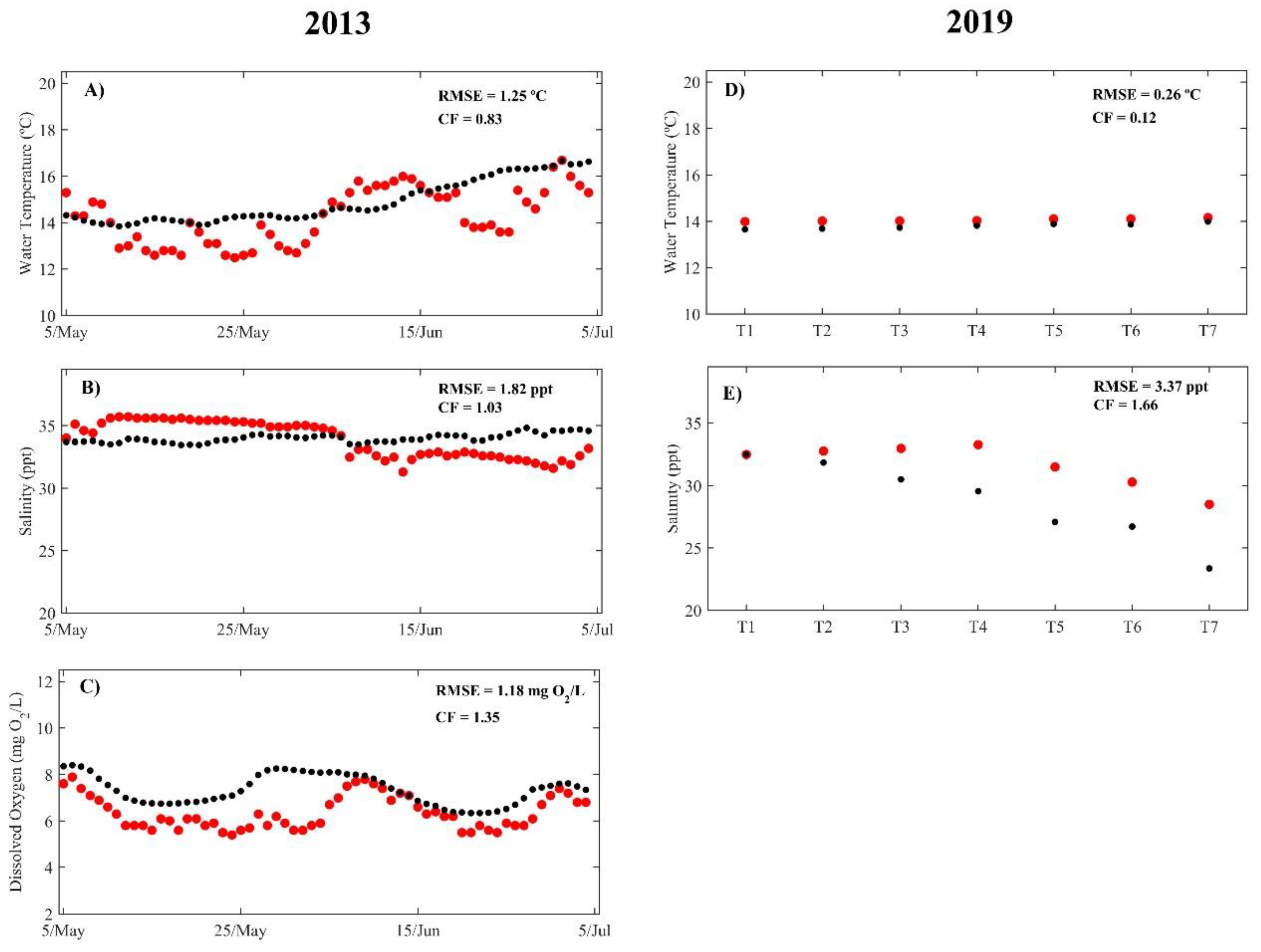
3.1. Model Calibration and Validation

The results obtained in the model calibration are presented in Table 2 and Table 3. Figure 4 shows the comparison between predicted and observed water temperature and salinity in transect 1 of the Minho and Lima estuaries, and Figure 5 shows the comparison between predicted and observed nitrates, orthophosphate, and dissolved oxygen in transect 1 of the Minho and Lima estuaries. Regarding the hydrodynamic module, a very good fit between model predictions and observed data was verified since the skill values were higher than 0.99 for most of the stations, the bias values were practically null, and the RMSE values were less than 10 cm, with the exception of Barra and Seixas stations. In these stations, a higher RMSE was observed, derived from the local geomorphological characteristics (enlargement and narrowing of the estuary) [87], which strongly modified the tidal fluxes. For salt and heat transport modules, Figure 4 shows the comparison between model predictions and observed water temperature and salinity in transect 1 of the Minho and Lima estuaries, respectively.
In Table 3, higher differences between predictions and observations were observed in the Minho estuary with a RMSE value of 1.34 °C for water temperature and 4.12 ppt for salinity. Regarding CF, it was observed that all values were between 0 and 1, which, according to Radach and Moll [82], represents a very good fit between predictions and observations. The higher values for the Minho estuary can be explained by the low resolution (~10 km) of forcing the open ocean boundary, by performing the simulations with a 2D model and by the existence of dams in both estuaries causing uncertainties in the freshwater inflows imposed, and by neglecting some small freshwater tributaries along the rivers (e.g., Louro, Tea, and Coura rivers). Finally, regarding the water quality module calibration results (Figure 5 and Table 3), the CF values indicated a good fit between predictions and observations (values between 1 and 2). It is found that the largest differences between model predictions and observed nitrate and orthophosphate occurred during periods of large river discharges and near the mouth, in both estuaries, since the concentration of nitrate and orthophosphate in estuaries is strongly influenced by river discharges. The RMSE value for dissolved oxygen was around 1.5 mg O2/L, and the CF value was around 2.5 (reasonable fit). Differences found between model predictions and observations may be due to several factors: (1) the module only considers algae as primary producers (e.g., cyanobacteria and microphytobenthos were not considered); (2) point discharges of pollutants along estuaries have not been inserted and may cause local changes in nutrient concentration and dissolved oxygen; and (3) geochemical processes and substances were not considered in the module. According to these results, the hydrodynamic and salt and heat transport modules had a good agreement between model predictions and observations. The water quality module demonstrated a reliable fit between predictions and observations, representing well the expected annual patterns of the substances under study, and the deviations of dissolved oxygen were very close to studies carried out by other authors [88,89].
The results obtained in the model validation are presented in Figure 6, showing once again that the model accurately represented the processes simulated in both estuaries. A good fit was obtained between predictions and observations for the two periods used to validate the model. For water temperature, a RMSE of 1.25 was obtained for 2013 data and of 0.26 for 2019, while an excellent fit was observed between predictions and observations based on CF values (ranging between 0–1). Regarding salinity, RMSE values of 1.82 and 3.37 were found for 2013 and 2019, respectively, and CF values were between 1 and 2, again showing a good fit between model predictions and observations. Finally, for the dissolved oxygen, a CF value of 1.35 (good fit) and a RMSE of 1.18 were obtained, which are, once more, in the accurate range of the studies referenced above.

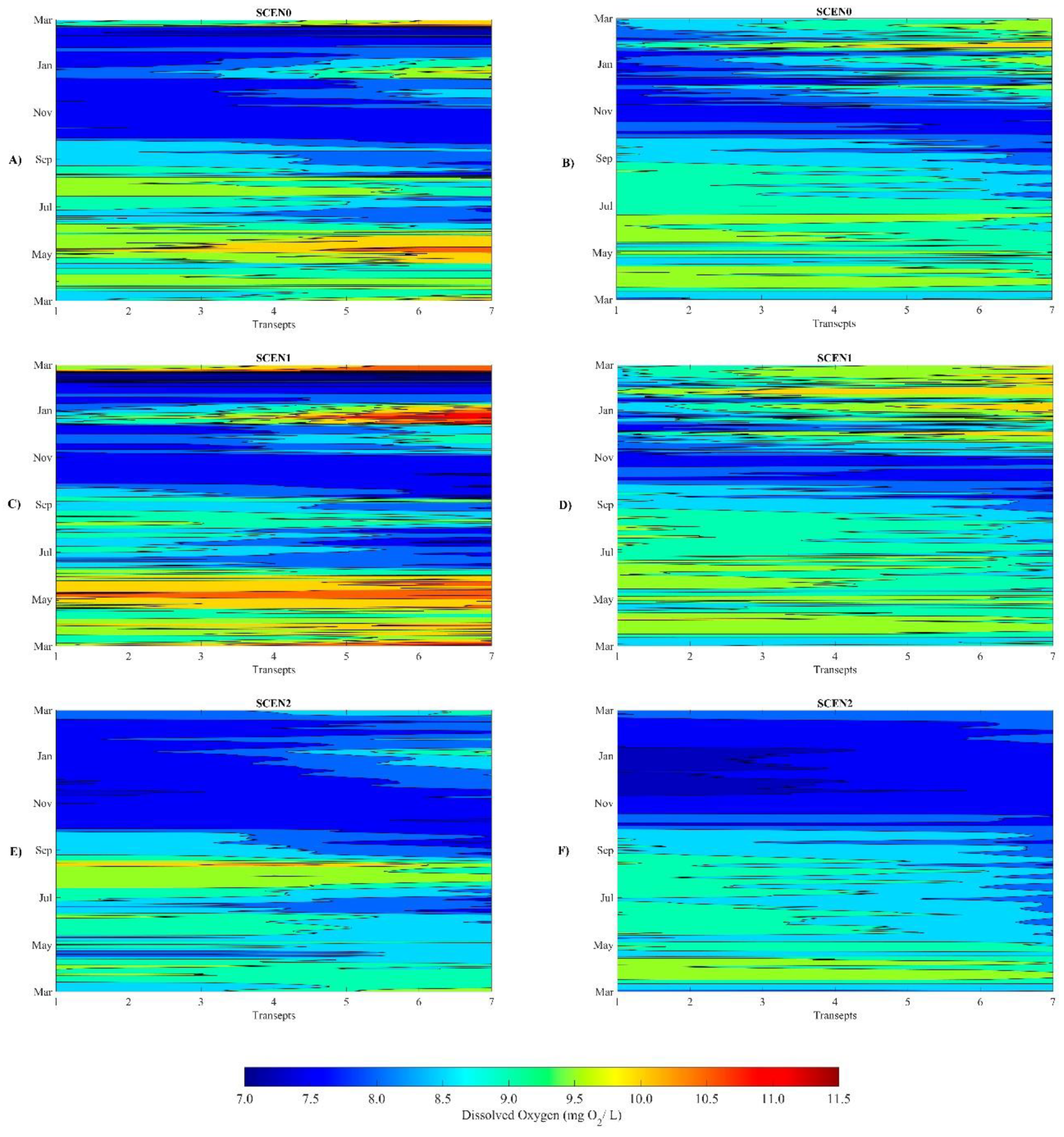
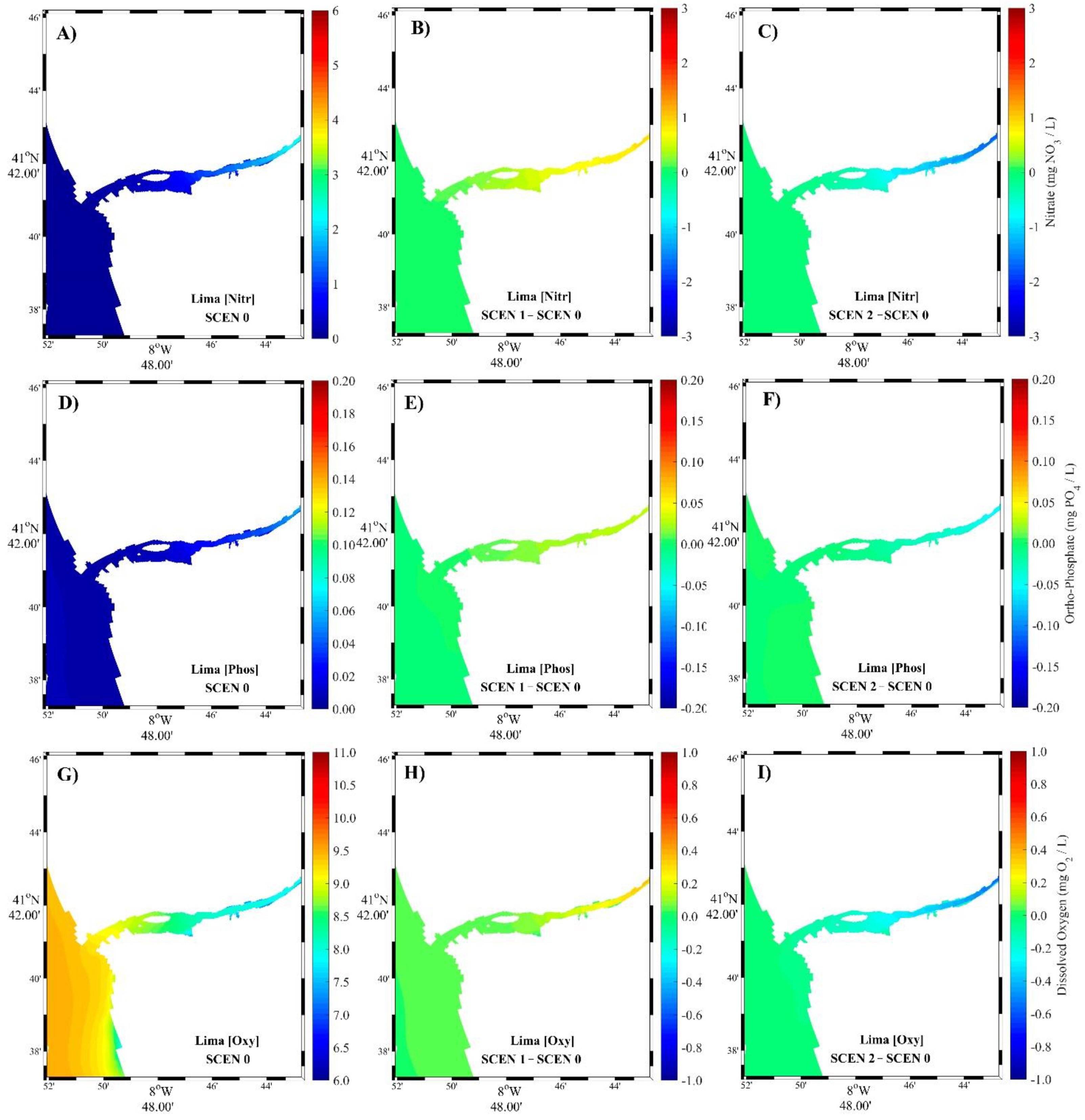
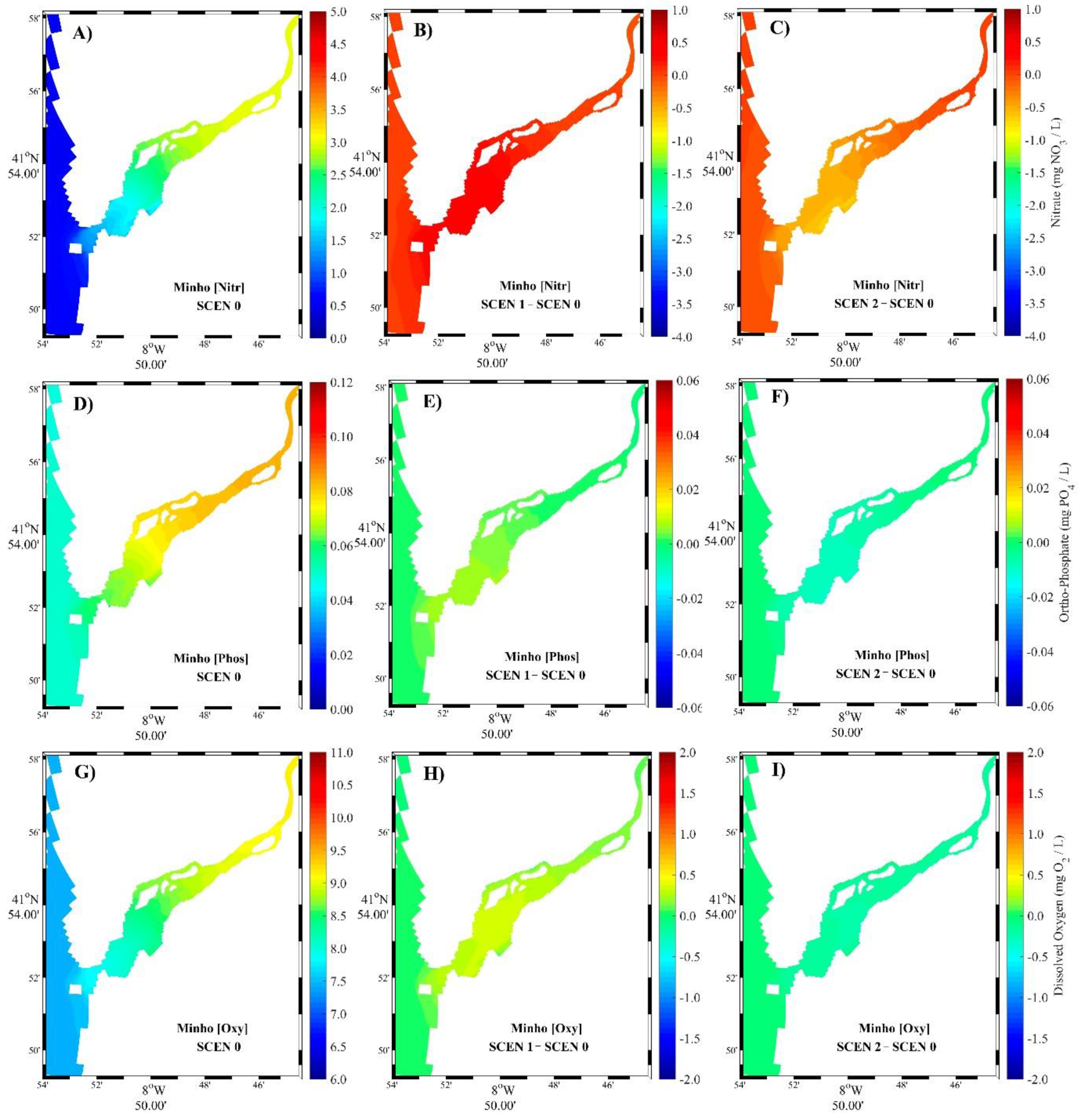
3.2. Model Scenarios

In order to analyse the periods with larger differences between scenarios, the annual longitudinal profiles of dissolved oxygen along the estuaries are represented in Figure 7 for each scenario. These profiles show that for both estuaries and for both scenarios, the greatest differences were observed in summer (21 June to 20 September 2012) and winter (21 December 2012 to 1 March 2013) seasons (e.g., Figure 7, representative of the dissolved oxygen variable throughout the year for different scenarios). In this way, a detailed analysis of all variables studied (salinity, water temperature, nitrate, orthophosphate, and dissolved oxygen) was carried out for these periods (Figure 8, Figure 9, Figure 10 and Figure 11 and Supplementary Figures S1–S4).

3.2.1. Summer Season

Figures S1 and S2 (refer to supplementary information) and Figure 8 and Figure 9 represent the average of the study variables for the summer season for the Minho and Lima estuaries, respectively. In the first column (baseline scenario) (Figures S1A and S2A), it was verified through the maps that the model represented an increasing longitudinal water temperature gradient (in the ocean it was possible to observe a mean water temperature of 18 °C and at the estuary heads a temperature of 23 °C). Regarding salinity (Figures S1D and S2D), a longitudinal gradient, with higher values of salinity in the oceanic area and lower in the river headwaters, was observed. Concerning nitrate (Figure 8A and Figure 9A) and orthophosphate (Figure 8D and Figure 9D), these nutrients were very close to zero in the oceanic area since these were mainly from terrestrial sources and river discharges, being absorbed and degraded as the water masses coming from the rivers are directed towards the coast. Finally, by analysing the average horizontal field of dissolved oxygen in both estuaries (Figure 8G and Figure 9G), the highest concentrations were found in the coastal zones and near the estuary mouths. The concentrations were around 9.5 mg O2/L at the mouth and 7.5 mg O2/L near the estuary head. The second column in Figure 8 and Figure 9 and Figures S1 and S2 represents the difference between the scenario of extreme discharge and the baseline scenario. In Figure S1B, it was observed that water temperature in the Minho estuary increased about 0.3 °C near the mouth, but it decreased about 0.6 °C in the upstream areas, whereas in the Lima estuary (Figure S2B) the differences were very close to zero. Regarding salinity (Figures S1E and S2E), it was found that both estuaries tended to become less saline because of the increase in river discharge, where the middle estuarine areas were the most affected. Since there was an increase in river discharge, there was an increase in the concentration of nutrients (nitrate and orthophosphate) inside the estuaries (Figure 8B,E and Figure 9B,E). The dissolved oxygen in the Minho estuary, in summer, decreased about 0.3 mg O2/L, and in the Lima estuary it decreased about 0.1 mg O2/L. In the third column, maps representing the difference between the ecological flow scenario and the baseline scenario were drawn. From these figures, an increase of 0.2 °C was found in the interior of the Minho estuary (Figure S1C), while in the Lima estuary, the differences were very close to zero (Figure S2C). A detailed analysis of the differences between the salinity for SCEN 2 and SCEN 0 show an unexpected salinity pattern in the Minho estuary (Figure S1F), since with ecological flows a higher saline intrusion was expected. This was not observed because the values of the ecological flows used for the summer season had fluvial discharges higher than those used in SCEN 0 (baseline scenario). Because of the aforementioned, a higher concentration of nutrients was observed in the ecological flow scenario (SCEN 2) than in the baseline scenario (SCEN 0).
For the Lima estuary, a larger saline intrusion was found (Figure S2F) since the river discharges for SCEN 2 were lower than those for the baseline scenario. In these conditions, the concentrations of nitrate and orthophosphate in the Lima estuary were lower (Figure 9C,F), leading to a decrease in the dissolved oxygen concentration (Figure 9I) inside the estuary (decrease of 0.2 mg O2/L).

3.2.2. Winter Season

In Figures S3 and S4 and Figure 10 and Figure 11, the averages of study variables (water temperature, salinity, orthophosphate, nitrate, and dissolved oxygen) for the winter season for the Minho and Lima estuaries are depicted, respectively. In Figures S3A and S4A, a predicted longitudinal gradient of water temperature was once again observed, but it was negative in the winter season (temperature of ocean water was higher than near the river mouth for both estuaries). Regarding nitrate and orthophosphate for both estuaries (Figure 10A,D and Figure 11A,D), these nutrients no longer have a concentration of zero in the oceanic area. The nitrate concentration was around 1 mg NO3/L, and the orthophosphate concentration was about 0.04 mg PO4/L. These concentrations were observed in the coastal zones because the rivers transport a large volume of nutrients in these conditions; therefore, exportation of nutrients towards the ocean occurs. Given that nutrient concentrations are relatively higher in the summer season, an increase in oxygen concentration was observed in both estuaries (Figure 10G and Figure 11G). In analysing the second column, representing the difference between extreme discharge and SCEN 0 (baseline) scenarios, water temperature in both estuaries (Figures S3B and S4B) was found to decrease about 0.5 °C near the mouth, while the temperature was almost constant in the areas upstream. Regarding salinity, in the maps representing the difference between SCEN 1 and SCEN 0 (Figures S3E and S4E), it was observed that both estuaries tended to become less saline, which was due to the increase of river discharges. This decrease in salinity and water temperature, as well as increased concentrations of nitrate and orthophosphate (increases of 0.9 and 0.01 mg PO4/L in both estuaries), will lead to an increase of dissolved oxygen in estuarine waters (increase 0.5 mg O2/L in the Minho estuary (Figure 10H) and 0.7 mg O2/L in the Lima estuary (Figure 11H)). Finally, in analysing the maps in the third column, representing the difference between ecological flow and baseline scenarios, it is noted that if ecological flows were discharged, there will be an increase in water temperature of 2 °C in the Lima estuary (Figure S4C) and of 0.5 °C in the Minho estuary (Figure S3C). Regarding salinity (Figures S3F and S4F), a larger saline intrusion was, once again, observed since the river discharges were very low. Given that river discharges of ecological flows were smaller compared to SCEN 0, a lower nutrient concentration was investigated (Figure 10C,F and Figure 11C,F), which caused a huge impact on the concentration of dissolved oxygen mainly in the Lima estuary. In fact, given the differences in river discharges between the baseline scenario and the drought scenario, a drastic decrease of 2 mg O2/L was found in the Lima estuary (Figure 11I), while in the Minho estuary (Figure 10I), only a decrease of 0.3 mg O2/L was observed.

4. Discussion

4.1. Model Calibration and Validation

The results of the water quality models normally showed significant deviations between predictions and observations when compared to the accuracy of the hydrodynamic models. This resulted in some model uncertainties, since these types of models present a greater complexity, and there were some limitations in the databases available for all variables under study.
In comparing the predictions with observations in model calibration (Figure 5A,B), the largest differences were found between predicted (black color) and observed (red color) nitrate in the winter months (December, January, and February) in both estuaries. This can be due to the fact that these periods are very rainy, and the river discharges are relatively high, providing transport of large amounts of nutrients (nutrients from human activities, agricultural field runoff, industrial effluents, and sewage from urban areas). For the remaining months, the model tended to underestimate concentrations. Regarding orthophosphate, the predictions followed the pattern of observations, but the model could not represent a few of the months because the data observed presented very high concentrations. These high concentrations indicated the possibility domestic effluents, industrial effluents, and sewage discharge existing along the estuaries [50], and these point sources were not accounted for in the numerical simulations performed. Another possibility of the model to present some deviations in nitrate may also be due to the denitrification rate, which may be faster than observed.
Regarding the observed differences between predicted and observed data of dissolved oxygen, the model reproduced the theoretical annual standard of dissolved oxygen since, in the summer months, there were lower concentrations of dissolved oxygen (higher consumption of oxygen than production), while in winter, there were higher concentrations of dissolved oxygen (higher production of oxygen than respiration (consumption)), and deviations were similar to other studies [88,89]. Another justification for this theoretical standard is that the higher the water temperature and salinity, the lower the concentration of oxygen; thus, in the summer months, where the water is warmer and more saline, lower concentrations of O2 are observed, but this could not be found in our observations. It is verified that, on average, the highest deviations were found near estuary mouths (Table 3) as well as in the winter months in both estuaries [83]. These differences are mainly due to the fact that there are large river discharges during the winter season and because a continuous temporary series was not imposed in the open water boundary for the period under study, but rather climatologic data were used.
With this, once again it can affirm that the differences found between predictions and observations may be due to several factors: (1) The model only considered algae as primary producers (e.g., cyanobacteria and microphytobenthos were not considered). If the activities of the remaining primary producers were also modeled, there could be some improvement in the adjustment between predicted and observed nutrient and dissolved oxygen concentrations, since there would be a higher nutrient consumption and higher photosynthesis [90]. (2) Point discharges of pollutants along estuaries were inserted and may cause local changes in nutrient concentration and dissolved oxygen. (3) Geochemical processes and substances were not considered in the model, which had large impacts on nutrient concentrations in the water column and in the mineralization processes. It is important to note that some of the factors mentioned may also have impact on the accuracy of the water quality module. Regarding the results obtained in the model validation, they were in the same range of accuracy as those determined during model calibration, demonstrating that the modules are able to accurately simulate the hydrodynamic and water quality processes under different and independent conditions. After this analysis, it can be assumed that the results of the model are reliable, and, in general terms, the model represents well the expected annual standards of the substances under study.

4.2. Model Scenarios

As mentioned earlier, water quality in estuaries is closely linked to the characteristics of their river basins, as river discharges bring solutes, nutrients, dissolved carbon, and particulate matter, and their concentrations may depend greatly on the hydrological, biological, and climatic patterns of each region. Therefore, the occurrence of extreme events changes the degree of dilution or concentration of nutrients, their residence time, and the distribution of saline water and fresh water inside the estuaries.
When studying the behaviour of nutrients in estuaries, it is necessary to consider the high complexity of all processes and substances and their interactions with each other. For this reason, biogeochemical studies of nutrients rarely take into account a wide variety of substances and processes [91], and this study was no exception.
Through the analysis of the water temperature variable, it was verified that with the increase of the fluvial discharges (SCEN1) there was, on average, a slight decrease in the water temperature, while with the decrease of the discharges (SCEN2), there was an increase in the water temperature both in the summer and winter. These changes in water temperature will have a direct impact on estuarine stratification, species distribution and abundance, growth and development of ectothermic organisms (organisms unable to regulate their own body temperature, depending on the ambient temperature), fish populations (which can cause death of species sensitive to water temperature variations), primary production, and, in turn, the concentration of dissolved oxygen in the water column (with increasing water temperature, microbial metabolism increases, and there is a reduction solubility of the dissolved gases). Although the increase in water temperature has some negative aspects, it is important to highlight that when there is low river discharge (drought event), the volume of water in the estuary decreases as a rule and can have positive effects, such as promoting germination and growth of macrophytes on exposed substrates [92].
Another variable that influences the primary production of estuarine fauna and flora, as well as their spatial distribution, is salinity, as it will affect species distribution and stratification. In SCEN1, it was observed that with the increase of river flow, the estuary in summer and winter will tend to have less brackish water, while the estuary will tend to have a greater saline intrusion in SCEN2.
Regarding nitrate and orthophosphate, the high concentrations observed by the discharges were mainly the result of anthropogenic activities in the river basins, and these concentrations can change drastically in a short time. Through the concentrations of these variables, it is possible to verify that, when there are major fluvial discharges, there are higher concentrations of nitrate and orthophosphate. From the analysis of SCEN1, it was verified that both estuaries presented higher concentrations of nutrients in relation to SCEN0. With the high concentrations of nutrients observed in SCEN1 and the increase of the velocity inside the estuaries, the dissolved oxygen concentration would be expected to increase in the estuaries, as these nutrients do not limit the photosynthesis process, and there is a higher re-aeration rate; however, this direct relationship was not always observed (e.g., in the summer). There are other factors/variables that control dissolved oxygen concentrations in the estuaries, such as the rate of oxygen consumption by consumers and decomposing beings (in summer, the rate of oxygen consumption overlaps with production, and in winter the opposite is observed), and the variables of water temperature and salinity also play an essential role in the concentration of dissolved oxygen (the higher the water temperature and the salinity, the lower the dissolved oxygen concentration).
Finally, in analysing the nutrients in SCEN2, a large decrease in nutrients present in both estuaries was verified. This was due to the reduction of river flow through the dams, which, together with the increase in water temperature and salinity observed inside the estuaries, provided a decrease in dissolved oxygen concentration and made the estuaries more anoxic (e.g., sharp decrease of 2 mg O2/ L in the Lima estuary). The fact that estuaries are more anoxic can seriously impact fauna and flora, as some species may die or be forced to migrate to other areas [93,94,95,96]. Many species are sensitive to large variations in the dissolved oxygen concentration [97,98,99,100].

5. Conclusions

The model Delft3D was applied to Minho and Lima estuaries in order to study the impact of climate change, especially extreme river discharge events, on nutrient dynamics in two estuaries subject to different hydrological regimes. Numerical experiments were conducted testing three scenarios with different river discharges.
The results for flood discharge (SCEN 1) suggest a reduced impact on the existing biota inside the estuaries (in both seasons), since there will be a higher concentration of dissolved oxygen in winter (+0.5 mg O2/L in the Minho estuary and +0.7 mg O2/L in the Lima estuary), and the decrease of oxygen is low in the summer (–0.3 mg O2/L in the Minho estuary and –0.1 mg O2/L in the Lima estuary). Regarding nutrient dynamics, there were no major differences between SCEN1 and baseline (SCEN 0) in both estuaries; however, nitrate and orthophosphate concentrations were higher than SCEN 0 because river discharge was also higher.
Concerning the ecological flow scenario (SCEN 2), it was concluded that with the reduction of river discharge, there will be a huge impact on the estuarine biota that exist in both estuaries and in nutrient dynamics. The Lima estuary, with the lower freshwater input, will be the most affected. There will be reduced nutrients supplied to the estuary, and it will become more anoxic (maximum decrease observed in the winter season of –2 mg O2/L), which may lead to the death or migration of some biological species and a reduction in the abundance and biomass of species with low mobility.
In summary, although the estuaries have some similar characteristics (e.g., latitudes and atmospheric conditions), differences in their hydrologic regimes induce dissimilar responses from local nutrient dynamics to the climate change impacts on freshwater inflows, especially under drought conditions. In fact, the smaller discharge of the Lima River results in higher impacts in the extreme drought events scenario (ecological flows, SCEN 2), with larger variations in the analysed variables.
Additionally, this research may also contribute to understanding the direct impact of building dams on rivers, since river inflows are controlled by dams in both estuaries in this study. In the future, significant precautions should be taken regarding the retention of fresh water in reservoirs located upstream of estuaries. The volume of river discharge will determine the ecological quality and health of the estuary as well as the availability of natural resources. A drastic reduction in discharge will have secondary consequences for the economic (e.g., aquaculture, pisciculture) and recreational (e.g., recreational fishing, scuba diving, tourism) sectors.
Finally, the use of water quality models nowadays is a powerful tool, as they provide valuable information to support stakeholders and authorities’ decisions. These models offer forecasts of estuarine dynamics and biogeochemistry, allow the isolated comprehension of different estuarine processes, and also serve to simulate possible scenarios of climate change in coastal water systems. It is important to note that, in these models, it is normal to have some degree of uncertainty and deviations from the observed data, since they are extremely intricate (complexity of the biogeochemical processes and their interactions). In addition, there are difficulties in obtaining high-quality databases.

Supplementary Materials

The following are available online at https://www.mdpi.com/2077-1312/7/11/412/s1, Figure S1: Mean water temperature (A–C), salinity (D–F) for Minho estuary in the summer season for the different scenarios, Figure S2: Mean water temperature (A–C), salinity (D–F) for Lima estuary in the summer season for the different scenarios, Figure S3: Mean water temperature (A–C), salinity (D–F) for Minho estuary in the winter season for the different scenarios, Figure S4: Mean water temperature (A–C), salinity (D–F) for Lima estuary in the winter season for the different scenarios.

Author Contributions

Conceptualization, V.H.O.; Formal analysis, V.H.O. and J.M.D.; Funding acquisition, F.M. and J.M.D.; Investigation, V.H.O.; Methodology, V.H.O., M.C.S., and J.M.D.; Software, M.C.S.; Supervision, M.C.S., F.M., and J.M.D.; Visualization, F.M.; Writing—original draft, V.H.O.; Writing—review & editing, V.H.O., M.C.S., F.M., and J.M.D.

Funding

The second author was funded by national funds (OE), through FCT—Fundação para a Ciência e a Tecnologia, I.P., in the scope of the framework contract foreseen in numbers 4, 5, and 6 of article 23 of the Decree-Law 57/2016 of 29 August, changed by Law 57/2017 of 19 July. Thanks are due to FCT/MCTES for the financial support to CESAM (UID/AMB/50017/2019), through national funds. This work was partially funded under the project AquiMap (MAR-02.01.01-FEAMP-0022), cofinanced by MAR2020 Program, Portugal 2020, and European Union though the European Maritime and Fisheries Fund.

Acknowledgments

Thanks to Luis R. Vieira from CIIMAR (Portugal) for providing the water quality data used in the model calibration.

Conflicts of Interest

The authors declare no conflict of interest.

References

  1. Glamore, W.C.; Rayner, D.S.; Rahman, P.F. Estuaries and Climate Change; Technical Monograph Prepared for the National Climate Change Adaptation Research Facility; Water Research Laboratory of the School of Civil and Environmental Engineering, UNSW: Sydney, Australia, 2016. [Google Scholar]
  2. Miranda, L.; Castro, B.; Kjerfve, B. Principios de Oceanografia Física de Estuários; Technical Report; Universidade de São Paulo: São Paulo, Brazil, 2002; 427p. [Google Scholar]
  3. Barbier, E.B.; Hacker, S.D.; Kennedy, C.; Koch, E.W.; Stier, A.C.; Silliman, B.R. The value of estuarine and coastal ecosystem services. Ecol. Monogr. 2011, 81, 169–193. [Google Scholar] [CrossRef]
  4. Nixon, S.W.; Ammerman, J.W.; Atkinson, L.P.; Berounsky, V.M.; Billen, G.; Boicourt, W.C.; Boynton, W.R.; Church, T.M.; Ditoro, D.M.; Elmgren, R.; et al. The fate of nitrogen and phosphorus at the land-sea margin of the North Atlantic Ocean. Biogeochemistry 1996, 35, 141–180. [Google Scholar] [CrossRef]
  5. Boynton, W.R.; Hagy, J.D.; Cornwell, J.C.; Kemp, W.M.; Greene, S.M.; Owens, M.S.; Baker, J.E.; Larsen, R.K. Nutrient Budgets and Management Actions in the Patuxent River Estuary, Maryland. Estuaries Coasts 2008, 31, 623–651. [Google Scholar] [CrossRef]
  6. Bukaveckas, P.A.; Isenberg, W.N. Loading, Transformation, and Retention of Nitrogen and Phosphorus in the Tidal Freshwater James River (Virginia). Estuaries Coasts 2013, 36, 1219–1236. [Google Scholar] [CrossRef]
  7. Doney, S.C.; Ruckelshaus, M.; Duffy, J.E.; Barry, J.P.; Chan, F.; English, C.A.; Talley, L.D. Climate change impacts on marine ecosystems. Estuaries 2002, 25, 149–164. [Google Scholar] [CrossRef] [PubMed]
  8. Trenberth, K.E.; Smith, L.; Qian, T.; Dai, A.; Fasullo, J. Estimates of the Global Water Budget and Its Annual Cycle Using Observational and Model Data. J. Hydrometeorol. 2007, 8, 758–769. [Google Scholar] [CrossRef]
  9. Joehnk, K.D.; Huisman, J.; Sharples, J.; Sommeijer, B.; Visser, M.P.; Stroom, M.J. Summer heatwaves promote blooms of harmful cyanobacteria. Glob. Chang. Biol. 2008, 14, 495–512. [Google Scholar] [CrossRef]
  10. Jones, A.; Haywood, J.; Boucher, O.; Kravitz, B.; Robock, A. Geoengineering by stratospheric SO2 injection: Results from the met Office HadGEM2 climate model and comparison with the Goddard Institute for Space Studies ModelE. Atmos. Chem. Phys. 2010, 10, 5999–6006. [Google Scholar] [CrossRef]
  11. IPCC. Part A: Global and Sectoral Aspects Contribution of Working Group II to the Fifth Assessment Report of the Intergovernmental Panel on Climate Change. In Climate Change 2014: Impacts, Adaptation, and Vulnerability; Cambridge University Press: Cambridge, UK; New York, NY, USA, 2014. [Google Scholar]
  12. Rosenzweig, C.; Casassa, G.; Karoly, J.D.; Imeson, A.; Liu, C.; Menzel, A.; Rawlins, S.; Root, L.T.; Seguin, B.; Tryjanowski, P. Assessment of observed changes and responses in natural and managed systems. Climate Change 2007: Impacts, Adaptation and Vulnerability. In Contribution of Working Group II to the Fourth Assessment Report of the Intergovernmental Panel on Climate Change; Parry, L.M., Canziani, F.O., Palutikof, P.J., an der Linden, J.P., Hanson, E.C., Eds.; Cambridge University Press: Cambridge, UK, 2007; pp. 79–131. [Google Scholar]
  13. Van Vliet, M.T.H.; Zwolsman, J.J.G. Impact of summer droughts on the water quality of the Meuse river. J. Hydrol. 2008, 353, 1–17. [Google Scholar] [CrossRef]
  14. Forbes, K.A.; Kienzle, S.W.; Coburn, C.A.; Byrne, J.M.; Rasmussen, J. Simulating the hydrological response to predicted climate change on a watershed in southern Alberta, Canada. Clim. Chang. 2011, 105, 555–576. [Google Scholar] [CrossRef]
  15. Falloon, P.D.; Betts, R.A. The impact of climate change on global river flow in HadGEM1 simulations. Atmos. Sci. Lett. 2006, 7, 62–68. [Google Scholar] [CrossRef]
  16. Xu, H.; Luo, Y. Climate change and its impacts on river discharge in two climate regions in China. Hydrol. Earth Syst. Sci. 2015, 19, 4609–4618. [Google Scholar] [CrossRef]
  17. Kennedy, V. Anticipated Effects of Climate Change on Estuarine and Coastal Fisheries. Fisheries 1990, 15, 16–24. [Google Scholar] [CrossRef]
  18. Ray, G.C.; Hayden, B.P.; Bulger, A.J.; McCormick-Ray, M.G. Effects of global warming on the biodiversity of coastal-marine zones. In Global Warming and Biological Diversity; Peters, R.L., Lovejoy, T.E., Eds.; Yale University Press: New Haven, CT, USA, 1992; pp. 91–104. [Google Scholar]
  19. Schwartz, F.J. Fishes affected by freshwater inflows and/or marine intrusions in North Carolina. J. Elisha Mitchell Sci. Soc. 1998, 114, 173–189. [Google Scholar]
  20. Wetz, M.S.; Yoskowitz, D.W. An ‘extreme’ future for estuaries? Effects of extreme climatic events on estuarine water quality and ecology. Mar. Pollut. Bull. 2013, 69, 7–18. [Google Scholar] [CrossRef]
  21. Hickel, W.; Mangelsdorf, P.; Berg, J. The human impact in the German Bight: Eutrophication during three decades (1962–1991). Helgoländer Meeresunters. 1993, 47, 243–263. [Google Scholar] [CrossRef]
  22. Voynova, Y.G.; Sharp, J.H. Anomalous Biogeochemical Response to a Flooding Event in the Delaware Estuary: A Possible Typology Shift Due to Climate Change. Estuaries Coasts 2012, 35, 943–958. [Google Scholar] [CrossRef]
  23. Wiltshire, K.H.; Manly, B.F.J. The warming trend at Helgoland Roads, North Sea: Phytoplankton response. Helgol. Mar. Res. 2004, 58, 269–273. [Google Scholar] [CrossRef]
  24. Luterbacher, J.; Werner, J.P.; Smerdon, J.E.; Fernández-Donado, L.; González-Rouco, F.J.; Barriopedro, D.; Ljungqvist, F.C.; Büntgen, U.; Zorita, E.; Wagner, S.; et al. European summer temperatures since Roman times. Environ. Res. Lett. 2016, 11, 024001. [Google Scholar] [CrossRef]
  25. Statham, P.J. Nutrients in estuaries—An overview and the potential impacts of climate change. Sci. Total Environ. 2012, 434, 213–227. [Google Scholar] [CrossRef]
  26. Amon, R.M.W.; Benner, R. Photochemical and microbial consumption of dissolved organic carbon and dissolved oxygen in the Amazon River system. Geochim. Cosmochim. Acta 1996, 60, 1783–1792. [Google Scholar] [CrossRef]
  27. Lange, R.; Staaland, H.; Mostad, A. The effect of salinity and temperature on solubility of oxygen and respiratory rate in oxygen-dependent marine invertebrates. J. Exp. Mar. Biol. Ecol. 1972, 9, 217–229. [Google Scholar] [CrossRef]
  28. Noyes, P.D.; McElwee, M.K.; Miller, H.D.; Clark, B.W.; Van Tiem, L.A.; Walcott, K.C.; Erwin, K.N.; Levin, E.D. The toxicology of climate change: Environmental contaminants in a warming world. Environ. Int. 2009, 35, 971–986. [Google Scholar] [CrossRef]
  29. Kattwinkel, M.; Kühne, J.-V.; Foit, K.; Liess, M. Climate change, agricultural insecticide exposure, and risk for freshwater communities. Ecol. Appl. 2011, 21, 2068–2081. [Google Scholar] [CrossRef]
  30. Hooper, M.J.; Ankley, G.T.; Cristol, D.A.; Maryoung, L.A.; Noyes, P.D.; Pinkerton, K.E. Interactions between chemical and climate stressors: A role for mechanistic toxicology in assessing climate change risks. Environ. Toxicol. Chem. 2013, 32, 32–48. [Google Scholar] [CrossRef]
  31. Preece, R.M.; Jones, H.A. The effect of Keepit Dam on the temperature regime of the Namoi River, Australia. River Res. Appl. 2002, 18, 397–414. [Google Scholar] [CrossRef]
  32. Cumming, G.S. The impact of low-head dams on fish species richness in Wisconsin, USA. Ecol. Appl. 2004, 14, 1495–1506. [Google Scholar] [CrossRef]
  33. Bredenhand, E.; Samways, M.J. Impact of a dam on benthic macroinvertebrates in a small river in a biodiversity hotspot: Cape Floristic Region, South Africa. J. Insect Conserv. 2009, 13, 297–307. [Google Scholar] [CrossRef]
  34. Wei, G.; Yang, Z.; Cui, B.; Li, B.; Chen, H.; Bai, J.; Dong, S. Impact of Dam Construction on Water Quality and Water Self-Purification Capacity of the Lancang River, China. Water Resour. Manag. 2009, 23, 1763–1780. [Google Scholar] [CrossRef]
  35. Fagherazzi, S.; Kirwan, M.L.; Mudd, S.M.; Guntenspergen, G.R.; Temmerman, S.; D’Alpaos, A.; van de Koppel, J.; Rybczyk, J.M.; Reyes, E.; Craft, C.; et al. Numerical models of salt marsh evolution: Ecological, geomorphic, and climatic factors. Rev. Geophys. 2012, 50. [Google Scholar] [CrossRef]
  36. Mieszkowska, N.; Firth, L.; Bentley, M. Impacts of climate change on intertidal habitats. MCCIP Sci. Rev. 2013, 2013, 180–192. [Google Scholar]
  37. Vargas, C.I.C.; Vaz, N.; Dias, J.M. An evaluation of climate change effects in estuarine salinity patterns: Application to Ria de Aveiro shallow water system. Estuar. Coast. Shelf Sci. 2017, 189, 33–45. [Google Scholar] [CrossRef]
  38. Mateus, M.; Vaz, N.; Neves, R. A process-oriented model of pelagic biogeochemistry for marine systems. Part II: Application to a mesotidal estuary. J. Mar. Syst. 2012, 94, 90–101. [Google Scholar] [CrossRef]
  39. Sousa, M.C. Modelling the Minho River Plume Intrusion into the Rias Baixas; Aveiro University and Porto University: Aveiro, Portugal, 2013. [Google Scholar]
  40. Pan, G.; Chai, F.; Tang, D.; Wang, D. Marine phytoplankton biomass responses to typhoon events in the South China Sea based on physical-biogeochemical model. Ecol. Modell. 2017, 356, 38–47. [Google Scholar] [CrossRef]
  41. Mattern, J.P.; Song, H.; Edwards, C.A.; Moore, A.M.; Fiechter, J. Data assimilation of physical and chlorophyll a observations in the California current system using two biogeochemical models. Ocean Model. 2017, 109, 55–71. [Google Scholar] [CrossRef]
  42. Neves, R. Numerical models as decision support tools in coastal areas. In Assessment of the Fate and Effects of Toxic Agents on Water Resources; Springer: Dordrecht, The Netherlands, 2007; pp. 171–195. [Google Scholar]
  43. APA Plano de Gestão da Região Hidrográfica do Minho e Lima—RH1—Relatório técnico—Comissão Europeia; Technical Report; Agência Portuguesa do Ambiente: Amadora, Portugal, 2012; 178p.
  44. PBH. Plano de Bacia Hidrográfica do Rio Minho—Relatório Final; Technical Report; Ministério do Ambiente e do Ordenamento do Território, Instituto da Água, Instituto Português: Lisboa, Portugal, 2001; 1704p. [Google Scholar]
  45. Delgado, A.; Taveira-Pinto, F.; Silva, R. Hydrodynamic and morphodynamic preliminary simulation of river Minho estuary. In Proceedings of the 6a Jornadas de Hidráulica, Recursos Hídricos e Ambiente; Faculty of Engineering, Uiversity of Porto: Porto, Portugal, 2011; pp. 113–126. [Google Scholar]
  46. Sousa, R.; Guilhermino, L.; Antunes, C. Molluscan fauna in the freshwater tidal area of the river Minho estuary, NW of Iberian Peninsula. Ann. Limnol. Int. J. Limnol. 2005, 41, 141–147. [Google Scholar] [CrossRef]
  47. Freitas, V.; Costa-Dias, S.; Campos, J.; Bio, A.; Santos, P.; Antunes, C. Patterns in abundance and distribution of juvenile flounder, Platichthys flesus, in Minho estuary (NW Iberian Peninsula). Aquat. Ecol. 2009, 43, 1143. [Google Scholar] [CrossRef]
  48. Azevedo, D.A.; Lacorte, S.; Viana, P.; Barceló, D. Occurrence of Nonylphenol and Bisphenol-A in Surface Waters from Portugal. J. Braz. Chem. Soc. 2001, 12, 532–537. [Google Scholar] [CrossRef] [Green Version]
  49. Castro, M.; Santos, M.M.; Monteiro, N.M.; Vieira, N. Measuring lysosomal stability as an effective tool for marine coastal environmental monitoring. Mar. Environ. Res. 2004, 58, 741–745. [Google Scholar] [CrossRef]
  50. Santos, S.; Vilar, V.J.P.; Alves, P.; Boaventura, R.A.R.; Botelho, C. Water quality in Minho/Miño River (Portugal/Spain). Environ. Monit. Assess. 2013, 185, 3269–3281. [Google Scholar] [CrossRef]
  51. Filgueiras, A.V.; Lavilla, I.; Bendicho, C. Evaluation of distribution, mobility and binding behaviour of heavy metals in surficial sediments of Louro river (Galicia, Spain) using chemometric analysis: A case study. Sci. Total Environ. 2004, 330, 115–129. [Google Scholar] [CrossRef] [PubMed]
  52. SNIRH Sistema Nacional de Informação de Recursos Hídricos. Available online: www.snirh.pt (accessed on 20 January 2018).
  53. Vale, L.M.; Dias, J.M. The effect of tidal regime and river flow on the hydrodynamics and salinity structure of the Lima estuary: Use of a numerical model to assist on estuary classification. J. Coast. Res. 2011, 64, 1604–1608. [Google Scholar]
  54. Barbosa, A.M.; Lousada, S.; Haie, N. Análise da Qualidade das Águas Superficiais de Ponte de Lima; Technical Report; Universidade do Minho: Braga, Portugal, 2004; 14p. [Google Scholar]
  55. Guimarães, L.; Gravato, C.; Santos, J.; Monteiro, L.S.; Guilhermino, L. Yellow eel (Anguilla anguilla) development in NW Portuguese estuaries with different contamination levels. Ecotoxicology 2009, 18, 385–402. [Google Scholar] [CrossRef] [PubMed]
  56. Cairrão, E.; Couderchet, M.; Soares, A.M.V.M.; Guilhermino, L. Glutathione-S-transferase activity of Fucus spp. as a biomarker of environmental contamination. Aquat. Toxicol. 2004, 70, 277–286. [Google Scholar] [CrossRef] [PubMed]
  57. Zacarias, N. Influência da Batimetria e do Caudal Fluvial na Propagação da Maré no Estuário do rio Minho; Technical Report; Universidade de Évora: Évora, Portugal, 2007; 81p. [Google Scholar]
  58. Vieira, L.R.; Guilhermino, L.; Morgado, F. Zooplankton structure and dynamics in two estuaries from the Atlantic coast in relation to multi-stressors exposure. Estuar. Coast. Shelf Sci. 2015, 167, 347–367. [Google Scholar] [CrossRef]
  59. Lesser, G.R.; Roelvink, J.A.; van Kester, J.A.T.M.; Stelling, G.S. Development and validation of a three-dimensional morphological model. Coast. Eng. 2004, 51, 883–915. [Google Scholar] [CrossRef]
  60. Bonamano, S.; Madonia, A.; Borsellino, C.; Stefanì, C.; Caruso, G.; De Pasquale, F.; Piermattei, V.; Zappalà, G.; Marcelli, M. Modeling the dispersion of viable and total Escherichia coli cells in the artificial semi-enclosed bathing area of Santa Marinella (Latium, Italy). Mar. Pollut. Bull. 2015, 95, 141–154. [Google Scholar] [CrossRef]
  61. Gils, J.; Ouboter, M.R.L.; De Rooij, N.M. Modelling of water and sediment quality in the Scheldt estuary. Neth. J. Aquat. Ecol. 1993, 27, 257–265. [Google Scholar] [CrossRef]
  62. Deltares. Simulation of Multi-Dimensional Hydrodynamic Flows and Transport Phenomena, Including Sediments [User Manual]; Deltares: Delft, The Netherlands, 2016; 702p. [Google Scholar]
  63. Deltares. Water Quality and Aquatic Ecology [User Manual]; Deltares: Delft, The Netherlands, 2016; 394p. [Google Scholar]
  64. Macmillan, D.S.; Beckley, B.D.; Fang, P. Monitoring the TOPEX and Jason-1 microwave tadiometers with GPS and VLBI Wet Zenith path delays. Mar. Geod. 2004, 27, 703–716. [Google Scholar] [CrossRef]
  65. Whitehead, P.; Bussi, G.; Hossain, M.A.; Dolk, M.; Das, P.; Comber, S.; Peters, R.; Charles, K.J.; Hope, R.; Hossain, M.S. Restoring water quality in the polluted Turag-Tongi-Balu river system, Dhaka: Modelling nutrient and total coliform intervention strategies. Sci. Total Environ. 2018, 631–632, 223–232. [Google Scholar] [CrossRef]
  66. Tomić, A.Š.; Antanasijević, D.; Ristić, M.; Perić-Grujić, A.; Pocajt, V. A linear and non-linear polynomial neural network modeling of dissolved oxygen content in surface water: Inter- and extrapolation performance with inputs’ significance analysis. Sci. Total Environ. 2018, 610–611, 1038–1046. [Google Scholar] [CrossRef] [PubMed]
  67. Gu, J.; Hu, C.; Kuang, C.; Kolditz, O.; Shao, H.; Zhang, J.; Liu, H. A water quality model applied for the rivers into the Qinhuangdao coastal water in the Bohai Sea, China. J. Hydrodyn. Ser. B 2016, 28, 905–913. [Google Scholar] [CrossRef]
  68. Kori, B.B.; Manojkumar, B.; Mise, S.R. Application of MIXPIPOX Model to Karanja River Water Quality. Procedia Earth Planet. Sci. 2015, 11, 260–265. [Google Scholar] [CrossRef] [Green Version]
  69. Kroeze, C.; Gabbert, S.; Hofstra, N.; Koelmans, A.A.; Li, A.; Löhr, A.; Ludwig, F.; Strokal, M.; Verburg, C.; Vermeulen, L.; et al. Global modelling of surface water quality: A multi-pollutant approach. Curr. Opin. Environ. Sustain. 2016, 23, 35–45. [Google Scholar] [CrossRef]
  70. Terry, J.A.; Sadeghian, A.; Baulch, H.M.; Chapra, S.C.; Lindenschmidt, K.-E. Challenges of modelling water quality in a shallow prairie lake with seasonal ice cover. Ecol. Modell. 2018, 384, 43–52. [Google Scholar] [CrossRef]
  71. Bui, H.H.; Ha, N.H.; Nguyen, T.N.D.; Nguyen, A.T.; Pham, T.T.H.; Kandasamy, J.; Nguyen, T.V. Integration of SWAT and QUAL2K for water quality modeling in a data scarce basin of Cau River basin in Vietnam. Ecohydrol. Hydrobiol. 2019, 19, 210–223. [Google Scholar] [CrossRef]
  72. Cebe, K.; Balas, L. Water quality modelling in kaş bay. Appl. Math. Model. 2016, 40, 1887–1913. [Google Scholar] [CrossRef]
  73. Doan, Q.T.; Nguyen, T.M.L.; Quach, T.T.T.; Tran, A.P.; Nguyen, C.D. Assessment of water quality in coastal estuaries under the impact of an industrial zone in Hai Phong, Vietnam. Phys. Chem. Earth Parts A/B/C 2019. [Google Scholar] [CrossRef]
  74. Feng, T.; Wang, C.; Hou, J.; Wang, P.; Liu, Y.; Dai, Q.; Yang, Y.; You, G. Effect of inter-basin water transfer on water quality in an urban lake: A combined water quality index algorithm and biophysical modelling approach. Ecol. Indic. 2018, 92, 61–71. [Google Scholar] [CrossRef]
  75. Nguyen, T.T.; Keupers, I.; Willems, P. Conceptual river water quality model with flexible model structure. Environ. Model. Softw. 2018, 104, 102–117. [Google Scholar] [CrossRef]
  76. Salleh, S.H.M.; Ahmad, A.; Mohtar, W.H.M.W.; Lim, C.H.; Maulud, K.N.A. Effect of projected sea level rise on the hydrodynamic and suspended sediment concentration profile of tropical estuary. Reg. Stud. Mar. Sci. 2018, 24, 225–236. [Google Scholar] [CrossRef]
  77. Wang, J.; Li, L.; He, Z.; Kalhoro, N.A.; Xu, D. Numerical modelling study of seawater intrusion in Indus River Estuary, Pakistan. Ocean Eng. 2019, 184, 74–84. [Google Scholar] [CrossRef]
  78. Xu, Y.; Cai, Y.; Sun, T.; Yang, Z.; Hao, Y. Coupled hydrodynamic and ecological simulation for prognosticating land reclamation impacts in river estuaries. Estuar. Coast. Shelf Sci. 2018, 202, 290–301. [Google Scholar] [CrossRef]
  79. Dias, J.M.; Lopes, J.F. Implementation and assessment of hydrodynamic, salt and heat transport models: The case of Ria de Aveiro lagoon (Portugal). Environ. Model. Softw. 2006, 21, 1–15. [Google Scholar] [CrossRef]
  80. Dias, J.M.; Sousa, M.C.; Bertin, X.; Fortunato, A.B.; Oliveira, A. Numerical modeling of the impact of the Ancão inlet relocation (Ria Formosa, Portugal). Environ. Model. Softw. 2009, 24, 711–725. [Google Scholar] [CrossRef]
  81. Atwater, M.A.; Ball, J.T. Computation of IR sky temperature and comparison with surface temperature. Sol. Energy 1978, 21, 211–216. [Google Scholar] [CrossRef]
  82. Radach, G.; Moll, A. Review of three-dimensional ecological modeling related to the North Sea shelf system. Part II: Model validation and data needs. Oceanogr. Mar. Biol. 2006, 44, 1–60. [Google Scholar]
  83. Oliveira, V.H. Coupled Modelling of the Minho and Lima Estuaries: Biochemical Response to Extreme Events and Interaction of Plumes Estuarine. Master’s Thesis, Aveiro University, Aveiro, Portugal, 2018; 132p. [Google Scholar]
  84. Hoegh-Guldberg, O.; Jacob, D.; Taylor, M.; Bindi, M.; Brown, S.; Camilloni, I.; Diedhiou, A.; Djalante, R.; Ebi, K.; Engelbrecht, F.; et al. Chapter 3: Impacts of 1.5 °C global warming on natural and human systems. In Global Warming of 1.5 °C; Geneva, Switzerland, 2018; pp. 175–311. Available online: http://pure.iiasa.ac.at/15518 (accessed on 13 November 2019).
  85. APA. Parte 2—Caracterização e Diagnóstico (Anexos)—Plano de Gestão da Região Hidrográfica do Minho e Lima (RH1); Technical Report; Agência Portuguesa do Ambiente: Amadora, Portugal, 2015; 92p. [Google Scholar]
  86. BOE. Anexo III. Plan Hidrológico de la Parte Española de la DH del MIÑO-Sil (2015–2021); Technical Report; Boletín Oficial del Estado: Catalonia, Spain, 2009; 28p. [Google Scholar]
  87. Reis, J.L.; Martinho, A.S.; Pires-Silva, A.; Silva, A.J. Assessing the influence of the river discharge on the Minho estuary tidal regime. J. Coast. Res. 2009, II, 1405–1409. [Google Scholar]
  88. Nagisetty, R.M.; Flynn, K.F.; Uecker, D. Dissolved oxygen modeling of effluent-dominated macrophyte-rich Silver Bow Creek. Ecol. Modell. 2019, 393, 85–97. [Google Scholar] [CrossRef]
  89. Suarez, V.V.C.; Brederveld, R.J.; Fennema, M.; Moreno-Rodenas, A.; Langeveld, J.; Korving, H.; Schellart, A.N.A.; Shucksmith, J. Evaluation of a coupled hydrodynamic-closed ecological cycle approach for modelling dissolved oxygen in surface waters. Environ. Model. Softw. 2019, 119, 242–257. [Google Scholar] [CrossRef]
  90. Vaz, L.; Mateus, M.; Serôdio, J.; Dias, J.M.; Vaz, N. Primary production of the benthic microalgae in the bottom sediments of Ria de Aveiro lagoon. J. Coast. Res. 2016, 75, 178–182. [Google Scholar] [CrossRef]
  91. Wangersky, P.J. Estuaries; Springer: Berlin/Heidelberg, Germany, 2006. [Google Scholar]
  92. Abrahams, C.; Brown, L.; Dale, K.; Edwards, F.; Jeffries, M.; Klaar, M.; Ledger, M.; May, L.; Milner, A.; Murphy, J.; et al. The Impact of Extreme Events on Freshwater Ecosystems. In Ecological Issues; Jones, I., Ed.; British Ecological Society: London, UK, 2013; p. 68. [Google Scholar]
  93. Bejda, A.J.; Studholme, A.L.; Olla, B.L. Behavioral responses of red hake,Urophycis chuss, to decreasing concentrations of dissolved oxygen. Environ. Biol. Fishes 1987, 19, 261–268. [Google Scholar] [CrossRef]
  94. Roman, M.R.; Gauzens, A.L.; Rhinehart, W.K.; White, J.R. Effects of low oxygen waters on Chesapeake Bay zooplankton. Limnol. Oceanogr. 1993, 38, 1603–1614. [Google Scholar] [CrossRef]
  95. Breitburg, D.L. Behavioral response of fish larvae to low dissolved oxygen concentrations in a stratified water column. Mar. Biol. 1994, 120, 615–625. [Google Scholar] [CrossRef]
  96. Breitburg, D.L.; Adamack, A.; Rose, K.A.; Kolesar, S.E.; Decker, B.; Purcell, J.E.; Keister, J.E.; Cowan, J.H. The pattern and influence of low dissolved oxygen in the Patuxent River, a seasonally hypoxic estuary. Estuaries 2003, 26, 280–297. [Google Scholar] [CrossRef]
  97. Lloyd, R. Effect of Dissolved Oxygen Concentrations on the Toxicity of Several Poisons to Rainbow Trout (Salmo Gairdnerii Richardson). J. Exp. Biol. 1961, 38, 447–455. [Google Scholar]
  98. Dauer, D.M.; Rodi, A.J.; Ranasinghe, J.A. Effects of low dissolved oxygen events on the macrobenthos of the lower Chesapeake Bay. Estuaries 1992, 15, 384–391. [Google Scholar] [CrossRef]
  99. Smith, K.J.; Able, K.W. Dissolved oxygen dynamics in salt marsh pools and its potential impacts on fish assemblages. Mar. Ecol. Prog. Ser. 2003, 258, 223–232. [Google Scholar] [CrossRef]
  100. Stevens, P.W.; Blewett, D.A.; Casey, J.P. Short-term effects of a low dissolved oxygen event on estuarine fish assemblages following the passage of hurricane Charley. Estuaries Coasts 2006, 29, 997–1003. [Google Scholar] [CrossRef]
Figure 1. Map of the study area (A). Minho (B) and Lima (C) estuaries with sampling transects (T1–T7) and location of the oceanic float (point “P”).
Jmse 07 00412 g001
Figure 2. Numerical bathymetry and tide gauge stations (red dots) used to extract sea surface elevation (A). Numerical grid (B).
Jmse 07 00412 g002
Figure 3. River flow values used for both scenarios in the Minho (A) and Lima (B) estuaries. To simplify, the visual comparison of the ecological flow values for the Lima estuary were multiplied by 10.
Jmse 07 00412 g003
Figure 4. Comparison between predicted (black dots) and observed (red dots) water temperature and salinity in transect 1 of the Minho (A,C) and Lima (B,D) estuaries, respectively.
Jmse 07 00412 g004
Figure 5. Comparison between predicted (black dots) and observed (red dots) nitrate, ortho-phosphate and dissolved oxygen in transect 1 of the Minho (A,C,E) and Lima (B,D,F) estuaries, respectively.
Jmse 07 00412 g005
Figure 6. Validation model comparison between predicted (black dots) and observed (red dots) water temperature (A), salinity (B), and dissolved oxygen (C) at point “P” shown in Figure 1, for the year 2013. Comparison between predicted (black dots) and observed (red dots) water temperature (D) and salinity (E) in the Lima estuary for the year 2019.
Jmse 07 00412 g006
Figure 7. Annual longitudinal profiles of dissolved oxygen along the different transects and scenarios for the Minho (A,C,E) and Lima estuaries (B,D,F).
Jmse 07 00412 g007
Figure 8. Mean nitrate (AC), orthophosphate (DF), and dissolved oxygen (GI) for the Minho estuary in the summer season for the different scenarios.
Jmse 07 00412 g008
Figure 9. Mean nitrate (AC), orthophosphate (DF), and dissolved oxygen (GI) for the Lima estuary in the summer season for the different scenarios.
Jmse 07 00412 g009
Figure 10. Mean nitrate (AC), orthophosphate (DF), and dissolved oxygen (GI) for the Minho estuary in the winter season for the different scenarios.
Jmse 07 00412 g010
Figure 11. Mean nitrate (AC), orthophosphate (DF), and dissolved oxygen (GI) for the Lima estuary in the winter season for the different scenarios.
Jmse 07 00412 g011
Table 1. Processes and substances selected for the water quality model.
SubstancesProcesses
Algae [Non-Diatoms]Potential minimum dissolved oxygen [OXYMin]
Net primary production and mortality [GroMrt_Gre]
Dissolved Oxygen [OXY]Potential minimum dissolved oxygen [OXYMin]
Uptake of nutrients by growth of alga [NutUpt_alg]
Variation of primary production within day [VAROXY]
Horizontal dispersion velocity dependence [HDisperVel]
Denitrification in water column [Denwat_NO3]
Nitrification of ammonium [Nitrif_NH4]
Reaeration of oxygen [RearOXY]
Composition [Compos]
Ammonium [NH4]Uptake of nutrients by growth of alga [NutUpt_alg]
Nitrification of ammonium [Nitrif_NH4]
Composition [Compos]
Nitrate [NO3]Uptake of nutrients by growth of alga [NutUpt_alg]
Denitrification in water column [DenWat_NO3]
Nitrification of ammonium [Nitrif_NH4]
Composition [Compos]
Orthophosphate [PO4]Uptake of nutrients by growth of alga [NutUpt_alg]
Ad(de)sorption of orthophosphorus to inorganic matter
Composition [Compos]
Table 2. Error values for tidal water levels.
EstuaryStationsRoot-Mean-Square Error (RMSE) (m)SKILLBias (m)
MinhoBarra0.1110.994−0.0068
Caminha0.0720.997−8.8287 × 10⁻⁴
Seixas0.2010.9740.0066
Vila Nova de Cerveira0.0480.998−4.203 × 10⁻⁴
Segadães0.0560.997−4.2299 × 10⁻⁴
LimaViana do Castelo0.0460.999−1.1767 × 10⁻⁴
Table 3. RMSE and cost function (CF) values for the transepts shown in Figure 1. RMSE unities are water temperature (°C), salinity (ppt), nitrate (mg NO3/L), orthophosphate (mg PO4/L), and dissolved oxygen (mg O2/L).
EstuaryVariableT1T2T3T4T5T6T7
RMSECFRMSECFRMSECFRMSECFRMSECFRMSECFRMSECF
MinhoWater Temperature1.340.301.000.210.810.200.870.170.780.171.010.251.450.26
Salinity4.120.271.160.050.540.020.370.020.270.010.400.020.590.04
Dissolved Oxygen1.723.041.572.751.422.691.582.351.581.881.401.731.521.81
Nitrate1.031.580.911.050.820.970.971.081.201.500.981.640.921.58
Orthophosphate0.050.660.090.830.140.800.130.730.120.730.090.570.080.75
LimaWater Temperature0.630.170.740.200.560.120.650.160.650.150.770.190.960.24
Salinity1.170.101.680.161.710.131.990.162.730.302.930.402.600.28
Dissolved oxygen1.682.651.422.131.522.361.431.751.461.651.391.691.321.34
Nitrate0.731.980.812.020.841.860.971.331.082.111.511.691.052.01
Orthophosphate0.051.090.051.100.051.070.170.560.200.710.170.800.130.98

