Biophysical Submesoscale Processes in the Wake of Hurricane Ivan: Simulations and Satellite Observations

Abstract

Tropical cyclone induced phytoplankton productivity is examined using a tropical cyclone version of the Coupled Ocean/Atmosphere Mesoscale Prediction System (COAMPS®). A four-component Nutrient–Phytoplankton–Detritus biological model is integrated into COAMPS to create a fully integrated air-ocean-wave-biology model. This study investigates the upper ocean physical and biological states before and after Hurricane Ivan traversed the central Gulf of Mexico, in mid-September 2004. Elevated concentrations of surface chlorophyll-a appear in the simulation two days after the passage of the tropical cyclone, and these results are spatially and temporally coherent with Moderate Resolution Imaging Spectroradiometer (MODIS) satellite data for this time period. Model results reveal enhancement of chlorophyll-a in submesoscale filaments on the periphery of a warm-core eddy that are dominated by large values of lateral strain and relative vorticity at the surface. The vertical circulation of the filament, with its associated upward vertical motion, permits surface ventilation of cold, nitrogen-rich water and subsequent stimulation of primary biological production. Here, we show for the first time that coupled biological-physical submesoscale processes may be simulated via a fully integrated air-sea-wave-biology tropical cyclone model that provides a mechanistic explanation of the conspicuous features revealed in satellite ocean color imagery following Ivan.

1. Introduction

This study utilizes the Naval Research Laboratory’s (NRL) Coupled Ocean Atmospheric Mesoscale Prediction System-Tropical Cyclone (COAMPS-TC) model to analyze the ocean’s coupled biological-physical response that occurred after the passage of Hurricane Ivan through the central Gulf of Mexico (GOM) in September 2004. An emerging paradigm for the oceanographic aftermath of such storm events in the GOM is that turbid waters overlying the continental shelf (overturned and well-mixed as a result of the storm) may be exported off of the shelf and into the pelagic GOM, along the peripheries of perturbed and intensified mesoscale circulation features. Whereas this offshore advection process may certainly occur following storm events [1,2] and at other times [3,4], the COAMPS-TC modeling results and satellite analysis presented herein demonstrate that the presumed horizontal advection that often appears in synoptic satellite images of the GOM (for example, the satellite ocean color chlorophyll-a product) may instead be due to submesoscale instabilities along the peripheries of larger circulation centers. Thus, the causative mechanism for the filament-like chlorophyll-a (Chla) features in the satellite images, may instead be due to the rapid ventilation of deeper, nutrient-rich waters within narrow areas of intense horizontal strain and relative vorticity.

Hurricane Ivan was an intense tropical cyclone (TC) in the central and eastern GOM from 14 September until landfall, at approximately 0700 UTC 16 September 2004, at Gulf Shores, Alabama. Hurricane Ivan’s extreme surface wind stress interacted with a cyclonic eddy, or cold-core eddy (CCE), that was located along the southern side of a large warm-core anticyclonic eddy, or warm-core eddy (WCE). Subsequently, a submesoscale filament (cross-axis distance less than 10 km) developed along the periphery of the WCE, and was a conspicuous feature within satellite estimates of Chla concentrations 3 to 4 days after the TC’s passage [1].

As discussed in reference [1], clear skies after Ivan’s passage across the GOM provided a unique opportunity to study both the physical (such as SST cooling) and biological changes of the upper ocean using satellite data from both passive and active sensors. Their study integrated sea surface height (SSH) data with satellite-derived SSTs and Chla, enabling a comparison of the ocean’s response within the CCEs and the WCE present along Ivan’s track. More generally, other studies have focused on the mechanisms of the ocean’s physical responses to TCs [5,6,7], as well as observational studies of TC impacts on surface phytoplankton and biological productivity [8,9,10,11]. However, this study primarily focuses on the submesoscale biophysical mechanisms associated with a narrow filament that emerged along the edge of an anticyclonic circulation feature following Ivan.

The fully integrated air-sea-wave-biology TC model used in this study permits simulation of the full dynamical ocean and biological interactions before and after a TCs passage. NRL’s TC model, COAMPS-TC, can simulate the intensity and structure of a TC, while producing realistic ocean and wave kinematic properties [12,13]. COAMPS-TC allows for interactions between the atmosphere, ocean, wave, and biology fields at every coupling time step of the model (6 min for this coupled simulation). COAMPS-TC, with an ocean biological sub-model, is able to provide post-TC biological constituent forecasts resulting from the track and intensity of a TC. These TC features, in turn, impact the coupled biophysical processes that result from TC-forced vertical mixing, entrainment, and upwelling. Herein, we examine the integrated air-sea-wave-biological simulation, in order to mechanistically explain the biophysical processes that manifest in the satellite observations, paying particular attention to a submesoscale cold filament that appears in satellite data in the days following Ivan.

In recent years, numerical ocean models have improved to the extent that submesocale filament structures can be resolved, allowing an assessment of their overall role in the physical processes of the upper ocean [14,15,16,17]. Recent literature studies have elucidated some of the processes of frontogenesis associated with growing submesocale filaments, similar to the one observed after the passage of Ivan. Submesoscale frontogenesis in the ocean can be compared to the classic paradigm of atmospheric frontogenesis, whereby a favorably aligned surface horizontal buoyancy gradient in a background deformation flow with a uniform strain rate has a rapidly growing magnitude [14]. It is suggested here that the primary background strain provided by mesoscale currents and eddies, such as the large WCE and LC in this case, provides the buoyancy gradients necessary to produce frontogenesis when subjected to a strong deformation of the flow field. Large values of strain at the surface are indicative of a strong ageostrophic overturning circulation that can generate relatively high vertical velocities beneath the surface. As the generation of this locally narrow region of high strain values continues to increase and become larger with time, a collapse of the along-front geostrophic balance occurs [17]. To re-establish geostrophic balance of the along-front current, a cross-frontal vertical circulation cell develops, with increased vertical velocities on both sides of the front. This vertical motion can then aid in raising the nutricline and provide nutrients for biological growth at the surface.

In this paper, it is suggested that the intense wind stresses of Hurricane Ivan, and the resulting inertial current oscillations, intensified the surface current deformation on the southern periphery of the WCE background flow, and the development of a submesoscale cold filament ensued after 16 September 2004. The colder, nutrient-rich waters stimulated surface primary production and resulted in a conspicuous filament feature, revealed by satellite data. In the following sections, we provide COAMPS model simulations and satellite observational data in order to resolve and analyze this biophysical submesoscale process.

2. Materials and Methods

2.1. COAMPS Setup and Initialization

Hurricane Ivan was a large and intense TC in the central and eastern GOM from 14 September, when it entered the southern GOM between western Cuba and the Yucatan Peninsula. The COAMPS-TC model setup for Hurricane Ivan consisted of a triple-nested atmospheric domain with 18, 6, and 2 km horizontal resolution and a total of 60 terrain-following vertical levels. The two inner nests translate in tandem with the cyclone’s vortex center, while the coarse atmospheric nest remains static. Spin-up (or hindcast period) of COAMPS-TC, with 12 h atmosphere and ocean data-assimilation cycles, commenced at 0000 UTC 1 September. Hurricane Ivan’s vortex, or eye, was initialized on 0000 UTC 10 September when the well-developed cyclone was located over the Caribbean Sea. The hindcast period provided the initial ocean and wave state as Ivan entered the GOM on 14 September. Three 72 h forecasts of Hurricane Ivan were generated: (1) at 1200 UTC 14 September (the period that Ivan moved through the GOM); (2) at 1200 UTC 17 September (the period just after landfall); and (3) at 1200 UTC 20 September (the period consisting of biological activity), to compare to satellite derived SST and Chla measurements. An example of COAMPS-TC wind speed, wind direction, and wave direction output for Hurricane Ivan is provided (Figure 1).

Atmospheric boundary conditions for each of the forecasts were provided by the Navy Operational Global Atmospheric Prediction System (NOGAPS) model [18], to aid in the hindcast of the synoptic scale meteorological environment that affected the intensity and track of the TC. The TC vortex initialization in the Navy Atmospheric Variational Data Assimilation System (NAVDAS) [19] used data that include center location, wind radii (distance of a certain wind speed threshold from the center of circulation), and intensity provided by the National Hurricane Center in Miami, FL and the Joint Typhoon Warning Center in Hawaii [20]. Each data assimilation cycle during the hindcast portion of the TC simulation in the atmospheric model was initiated using the prior 12 h forecast as background, incorporating quality-controlled observations from radiosondes, aircraft, satellites, ships, and surface stations.

The Navy Coastal Ocean Model (NCOM) [21] configuration included the biology module and consisted of a 2 km resolution nest that encompassed the entire GOM and Caribbean Sea. The ocean grid consisted of 50 vertical levels, with 36 sigma layers between the surface and 190 m depth (which are bottom-following in water shallower than 190 m), and 14 fixed-depth layers between 190 m and the maximum depth of 5500 m. Bathymetric data were obtained from the Navy’s two-minute resolution Digital Bathymetric Data Base (DBDB2). Initial and boundary conditions for NCOM were from a global version of NCOM [22]. The Navy Coupled Ocean Data Assimilation (NCODA) system’s three-dimensional variational scheme (3DVAR) ingests observational and global ocean data, including quality-controlled satellite, ship, profiler, and Modular Ocean Data Assimilation System (MODAS) synthetic profile data [23] for each update cycle during the hindcast portion of the simulation. The ocean model includes tides and river inflows, as well.

Although wave interactions with the biology are beyond the scope of this study, incorporating the Simulating Waves Nearshore (SWAN) model feedback to the atmosphere was necessary to aid in hindcasting the intensity of Hurricane Ivan [13]. Wave interactions with the ocean currents, including the Stokes’ drift current, impacted upper-ocean mixing, especially near the surface; therefore, wave action imparted a contribution (albeit small when wave action is minimal) to the overall vertical distribution of biological constituents in the water column during the biological production phase of the simulation. The SWAN model configuration consisted of one 8 km resolution grid that encompassed the same geographic area as the NCOM grid.

2.2. Biological Module in COAMPS-TC

The ocean biological module integrated into the COAMPS-TC for this study is a four-component Nutrient–Phytoplankton–Detritus (NPD) model (phytoplankton, nitrate nitrogen, ammonium nitrogen, and particulate detritus nitrogen). First, nitrate is initialized from observed temperature-to-nitrate relationships [24]. The subsequent nitrogen cycling proceeds as simulated phytoplankton biomass assimilate nitrogen (constrained by light- and nutrient-limited growth calculations) and is then subject to grazing/mortality terms. Nitrogen-containing particulate detritus sinks and is subject to respiration. Mortality and respiration contribute to the ammonium pool, and the cycle is completed via light-inhibited nitrification. A detailed description of the biological module integrated into the COAMPS can be found in reference [25]. The biological constituents were transported as tracers by the ocean circulation model at each time step.

2.3. Satellite Observations

MODIS (Aqua) sensor data for the Gulf of Mexico during boreal summer were obtained from the NASA Atmosphere Archive & Distribution System (LAADS) Distributed Active Archive Center (DAAC). These Level 1 data were processed by NRL via the Automated Optical Processing System (AOPS) [26]. Over 64 inversion algorithm products are produced by the AOPS, and this includes the NASA standard surface chlorophyll-a product [27] for the MODIS sensor, which is a blend of the OC3M band ratio algorithm and a modified version of the chlorophyll-a algorithm for oligotrophic waters [28]. The AOPS performs the appropriate atmospheric correction to also produce Remotely sensed reflectance (Rrs; sr⁻¹) for the MODIS ocean color bands.

Quantitative true color reconstruction from Rrs products is based on the satellite colorimetry method [29,30]. The Rrs products were subjected to a cubic spline interpolation procedure in order to reconstruct the hyperspectral reflectance signature (Δλ= 1 nm, 400–700 nm) for each pixel. The interpolated reflectance spectra (ρ_w= Rrs(λ) π) were integrated (via the Reimann sum approximation) with the CIE (International Commission on Illuminations) 1931 standard color matching functions, to produce the X,Y and Z color primaries. CIE chromaticity coordinates were converted to standard RGB, for display as JPEG images. As demonstrated herein, true color is a useful analysis tool to distinguish water masses (for example, shelf waters versus pelagic) in cases where standard inversion algorithm products (such as surface chlorophyll) are less informative.

3. Results

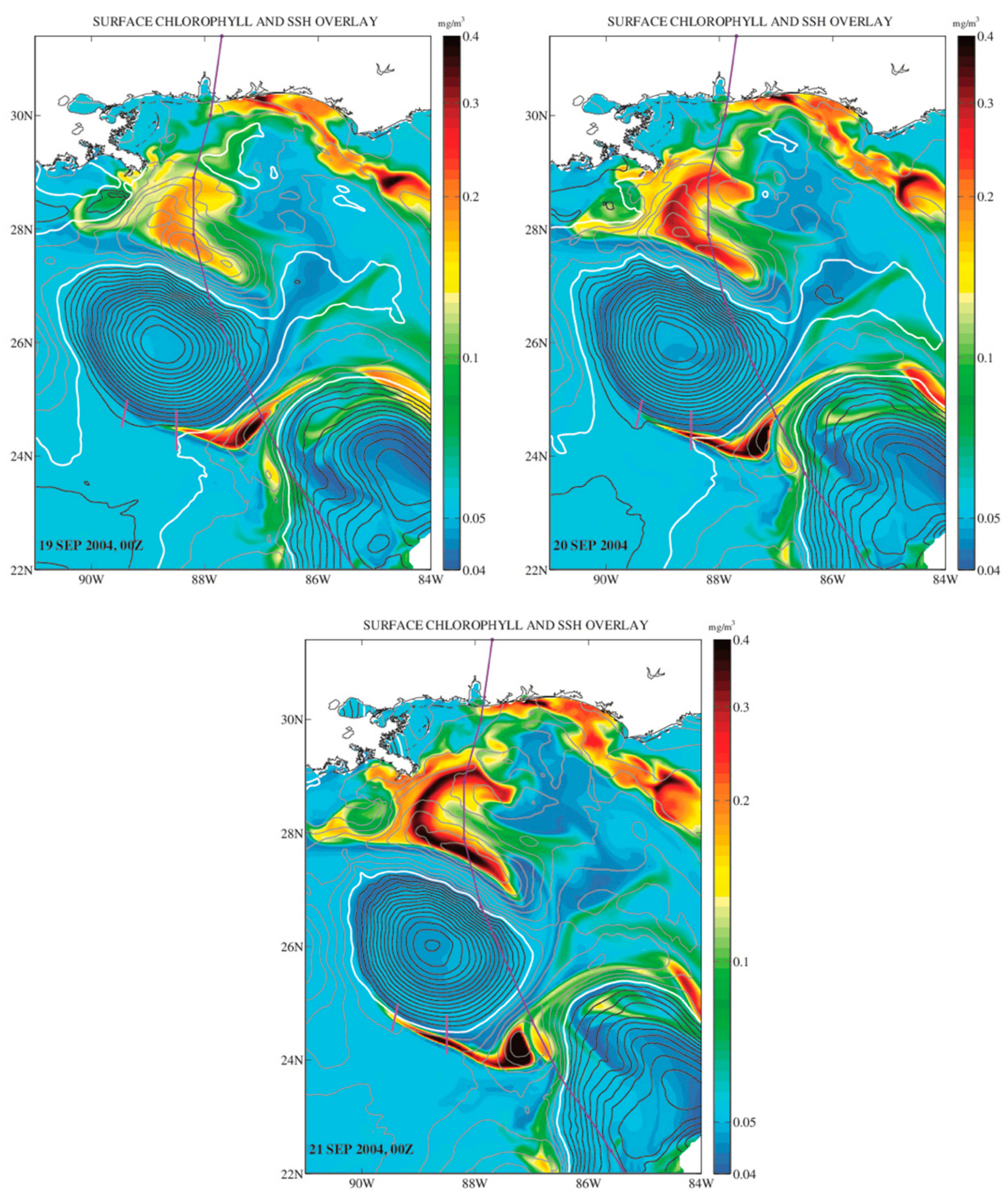
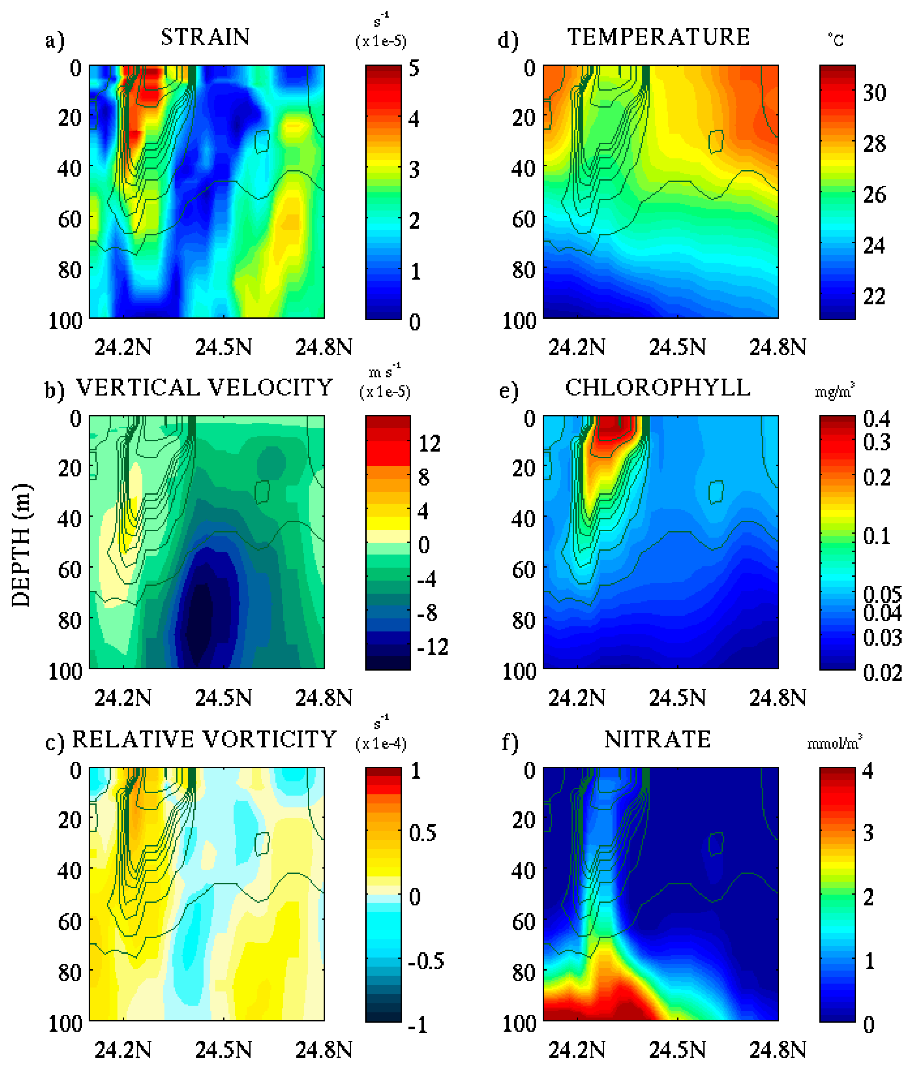
3.1. COAMPS Results and Development of Submesoscale Structures

Complex interactions between Hurricane Ivan and both the LC and WCE ensued after Hurricane Ivan entered the Gulf of Mexico on 14 September 2004. The COAMPS sea surface height (SSH) pre-storm conditions on 13 September 2004 show a large WCE over the north central GOM, with the LC to the south and east of the WCE (Figure 2a). Whereas the hindcast COAMPS mesoscale SSH field is constrained by satellite altimetry observations, the COAMPS SSH is an accurate representation of pre-storm conditions in the Gulf. After Ivan’s passage, COAMPS revealed a distinct CCE presence at approximately 87° W and 25° N on the southern outer edge of the WCE, on 17 September 2004 (Figure 2b). In addition to the CCE, the TC-induced SST cooling in the COAMPS simulations, associated with Ivan’s wind forcing and shear stresses, primarily occurred outside of the WCE and LC regions (Figure 2b). Inside the WCE and LC anticyclonic circulation features, warm waters extend to greater depths, and thus ameliorate the upward entrainment mixing to the surface and surface cooling impact of the TC passage (Figure 3a). Elsewhere, the SST cooling was largely to the right of Ivan’s track, which is typical during a TC passage [31]. The CCE positioned along the Ivan track between the WCE and LC appears to be an epicenter of particularly intense SST cooling (Figure 3b), with SSTs reducing to near 27 °C on 17 September.

In the days following the passage of Hurricane Ivan over the Gulf of Mexico, a narrow filament of cooler SSTs developed within the COAMPS SST fields along the southern flank of the WCE to the west of the CCE (Figure 3b–d). It is important to note that this cold filament develops secondary to the initial SST cooling process associated with the TC wake (Figure 3b). This cold filament continued to elongate westward around the WCE over the next few days (Figure 3a–d). By 20 September 2004, a fully developed narrow filament of cooler SSTs had developed around the southern periphery of the WCE (Figure 3d). It is tempting to attribute this cold filament growth to simple horizontal advection of colder surface waters around the anticyclonic circulation center, however, the propagation speed of the 28 °C surface isotherm is approximately two to three times more rapid than what would be permissible given the simulated surface currents along the WCE periphery.

This cold filament instead appears to be a baroclinic instability that is consistent with submesoscale dynamics, i.e., it has a cross-axis scale less than 10 km in width where rotational dynamics would begin to be irrelevant (Rossby number O(1)) [14,32]. This is in contrast to larger mesoscale flows (such as the WCE) that are characterized by small Rossby numbers O(10⁻²–10⁻¹) (Ro = ζ /f, where relative vorticity, ζ = dv/dx-du/dy, and f is the Coriolis parameter). Mesoscale flows are largely two-dimensional, and the dynamics at mesoscales are strongly influenced by the Earth’s rotation. In contrast, submesoscale processes typically have large Rossby numbers and are the result of baroclinic instabilities and/or surface forcing (they can also interact and generate submesoscale features). They are localized regions of intense, usually positive, relative vorticity that attain values as large as (or larger than) the Coriolis or planetary vorticity [32].

In typical mesoscale circulations, the elevated vorticity is distinct from areas with large lateral strain rates [33,34]. However, within ocean submesoscale dynamics, the largest horizontal strain rates, St = ((du/dx – dv/dy)² + (dv/dx + du/dy)²)^1/2 and vorticity occur concomitantly in filaments and are similar in magnitude [35]. Before the passage of Hurricane Ivan, the mesoscale WCE was dominated by anticyclonic vorticity in the center of the vortex, while uniformly low values of horizontal strain surrounded the outer edge or periphery. For the fully developed filament on 20 September 2004, the horizontal strain rate and vorticity were calculated at the surface and are shown in Figure 4. The maximum horizontal strain (shaded region in Figure 4a) was 1.7 × 10⁻⁴ s⁻¹ and the maximum relative vorticity (Figure 4b) was 1.6 × 10⁻⁴ s⁻¹ at this time. Since the horizontal strain and vorticity have the same magnitude, and their maximum values were co-located with the filament, this agrees with the literature description of submesoscale filaments [36]. The relative vorticity also exceeds the planetary vorticity (~ 0.6 × 10⁻⁴ s⁻¹) at this location.

Similarly, some studies use the calculation of the Okubo–Weiss parameter [37], St² - ζ², that is shown in Figure 5 on 13 and 20 September 2014 0000 UTC. Before Hurricane Ivan, the WCE is dominated by vorticity in the interior (negative OW) and moderate values of strain on the edges (positive OW; Figure 5a). After the storm, the high strain rate and positive Okubo–Weiss parameter values on the edge of the WCE are interspersed with elevated vorticity nodes (strong negative OW) that indicate a submesoscale strain-induced process acting on the buoyancy gradient. Quantitatively, in terms of strain and vorticity at the ocean surface, this process is described as frontogenesis [37]. The wind stresses associated with Ivan enhanced the shear along the horizontal buoyancy gradient on the edge of the WCE, a process potentially perpetuated over time by inertial current oscillations. Baroclinic instability in the presence of this enhanced shear caused a loss of geostrophic balance, which subsequently generated an ageostrophic or vertical secondary circulation to restore the geostrophic balance, and is described below.

We note that before Ivan (Figure 5a), there is significant strain and vorticity along the western side of the LC as it enters the GOM. This is likely due to LC interaction with the Yucatan continental shelf (Campeche Bank). Whereas this manuscript is focused upon the open ocean filament that appears following Ivan, both COAMPS and satellite data show elevated biological activity associated with the LC as it moves past the Campeche Bank, likely due to upwelling and shelf–current interactions [38].

To further analyze the submesoscale filament dynamics, it is also necessary to examine the filament in the meridional two-dimensional plane. A day after Hurricane Ivan’s U.S. landfall, the simulated vertical temperature gradient on the southern edge of the WCE was still largely intact and unremarkable. However, on 20 September the submesoscale filament had emerged along the WCE border and the vertical cross-section (24.5° N to 25° N; ~89.6° W) of horizontal strain (Figure 6a) shows elevated strain values from the surface to 30 m depth. As mentioned previously, the relative vorticity is enhanced and co-located with the maximum strain (Figure 6a,c). At this time, the Rossby number associated with the filament is of O(1) (R_o = ζ/f) and the secondary ageostrophic circulation produced vertical velocities that were an order of magnitude stronger than the background vertical velocities outside the filament (Figure 6b). It has been shown that the vertical velocities associated with O(1) Rossby number dynamics are asymmetric, with the downwelling being more intense than the upwelling in these submesoscale filaments [35]. As shown in Figure 6b, the downward (negative) vertical velocity is approximately four times stronger than the maximum upwelling (positive) vertical velocity. In addition, this concomitant dipole of positive and negative vertical velocity beneath the largest values of surface strain (Figure 6a,b) indicates frontogenesis at and near the surface along the deformation zone on the outer edge of the WCE.

The resulting biophysical property distributions are in accord with this emerging ageostrophic disturbance. Colder, subsurface waters are ventilating at the point of maximum surface strain (Figure 6d). The chlorophyll field (Figure 6e) is undergoing emerging excitation at the point of maximum strain, as the surface nitrate (Figure 6f) responds in accord with the physical circulation.

Farther east (~88.2 W), the simulated cold filament is more advanced in its biophysical evolution. Beneath the maximum horizontal strain value (Figure 7a), there is a horizontal dipole of positive/negative vertical velocities, with a bias towards stronger downwelling velocities (Figure 7b). Vertical velocities correspond to calculated values of relative vorticity (Figure 7c). Surface chlorophyll values have entered the mesotrophic range (~0.4 mg m⁻³) and a conspicuous column of nitrate extends upwards from ~ 80 m depth to the surface (Figure 7e–f). Mesotrophic waters are defined herein as 0.2 ≤ Chla ≤ 2.0, and oligotrophic and eutrophic waters are below and above this range, respectively.

The overall pattern of convergence and divergence at both the surface and at depth are indicative of ageostrophic circulation and coincide with the vertical velocity pattern within the filament (Figure 6b, Figure 7b). Whereas these model results are dynamically consistent with the literature description of submesoscale frontogenesis [14,35,39], descriptions of mesoscale–submesoscale coupling [16] and submesoscale cold filament frontogenesis [40], or “filamentogenesis” [41] are pertinent. The initial wind stress perturbation results in an amplification of mesoscale circulation patterns, with respect to the LC and WCE, and this subsequently results in the evolution of dynamically submesoscale cold filaments along the peripheries of the anticyclonic circulation centers.

The synoptic view of the simulated Chla (cold) filament evolution (Figure 8) over 2 days (19 to 21 September) suggests propagation velocity (with respect to excitation of the simulated chlorophyll field above background) of ~1.2 m s⁻¹. Simulated current velocities on the outer edge of the WCE during this time period are on the order of ~ 0.4–0.6 m s⁻¹. Thus, although the filament takes on the appearance of a horizontally advective surface process, the simulation shows that it is dynamical, and the cold water, high nutrient perturbation within the filament largely originates from depth. Simulated surface expression of colder, subsurface waters takes place within narrow areas of maximum horizontal strain, as opposed to areas of maximum horizontal current velocities.

In addition to the filament evolution and the CCE, the COAMPS biophysical results show elevated Chla along the edges of the LC, a larger area north of the WCE, and shelf upwelling in the Florida Panhandle region (Figure 8). These features correspond to satellite images (Section 3.2), however, we focus herein on the southerly filament, as its development appears in the simulation to occur almost entirely after the TC has passed.

One day after the initial filament cross-sections (Figure 6 and Figure 7) on 21 September, the filament cross-section along ~ 89.6° W (Figure 9 and, by comparison, Figure 6) shows the rapidly advancing development of the chlorophyll and cold temperature filament. Upward vertical velocities, horizontal strain, and relative vorticity (Figure 9a–c) are consistent with vertical excursions of lower temperature water and elevated nitrate concentrations (Figure 9d,f). A narrow filament of mesotrophic chlorophyll then emerges at the surface (Figure 9e).

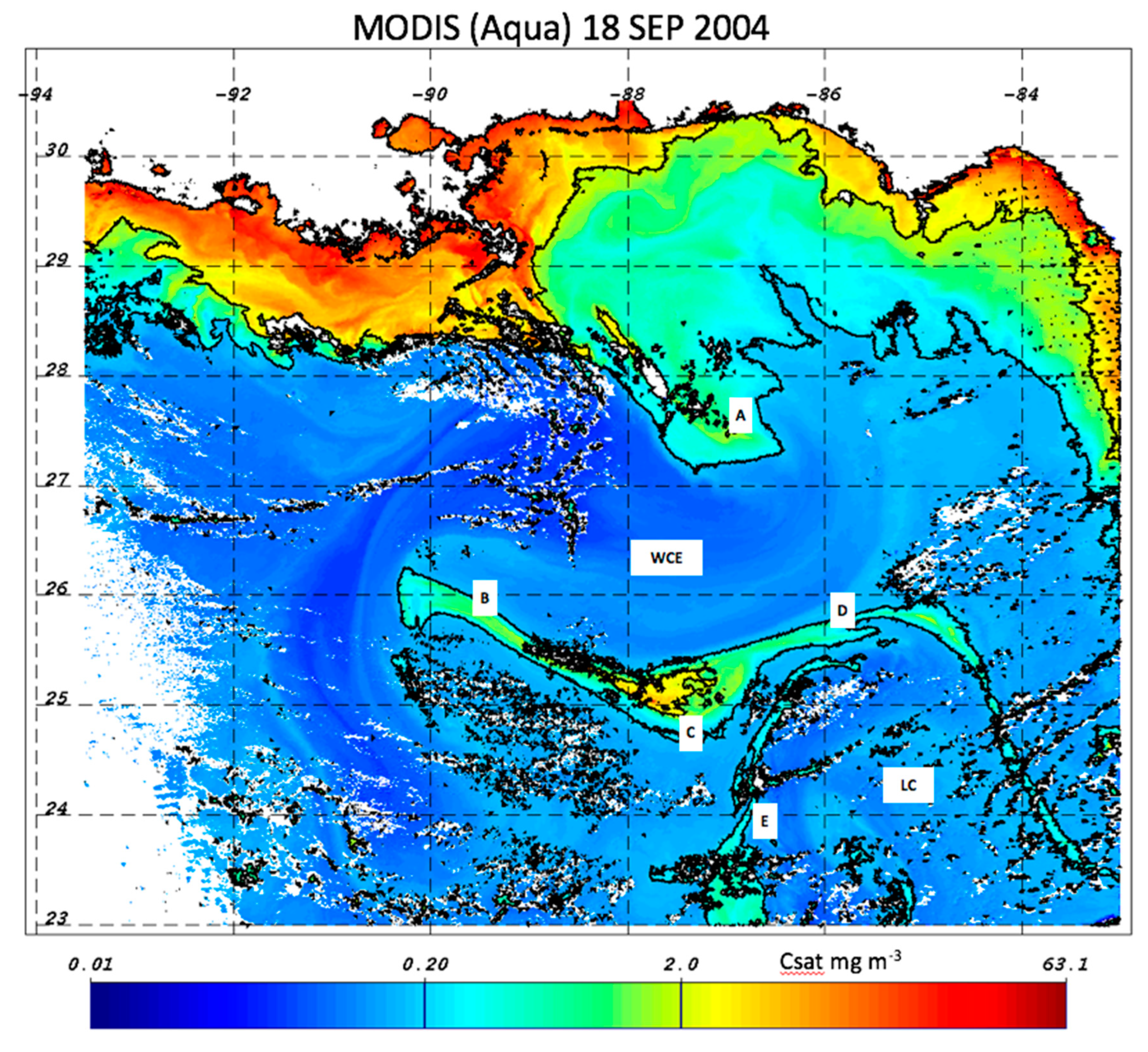
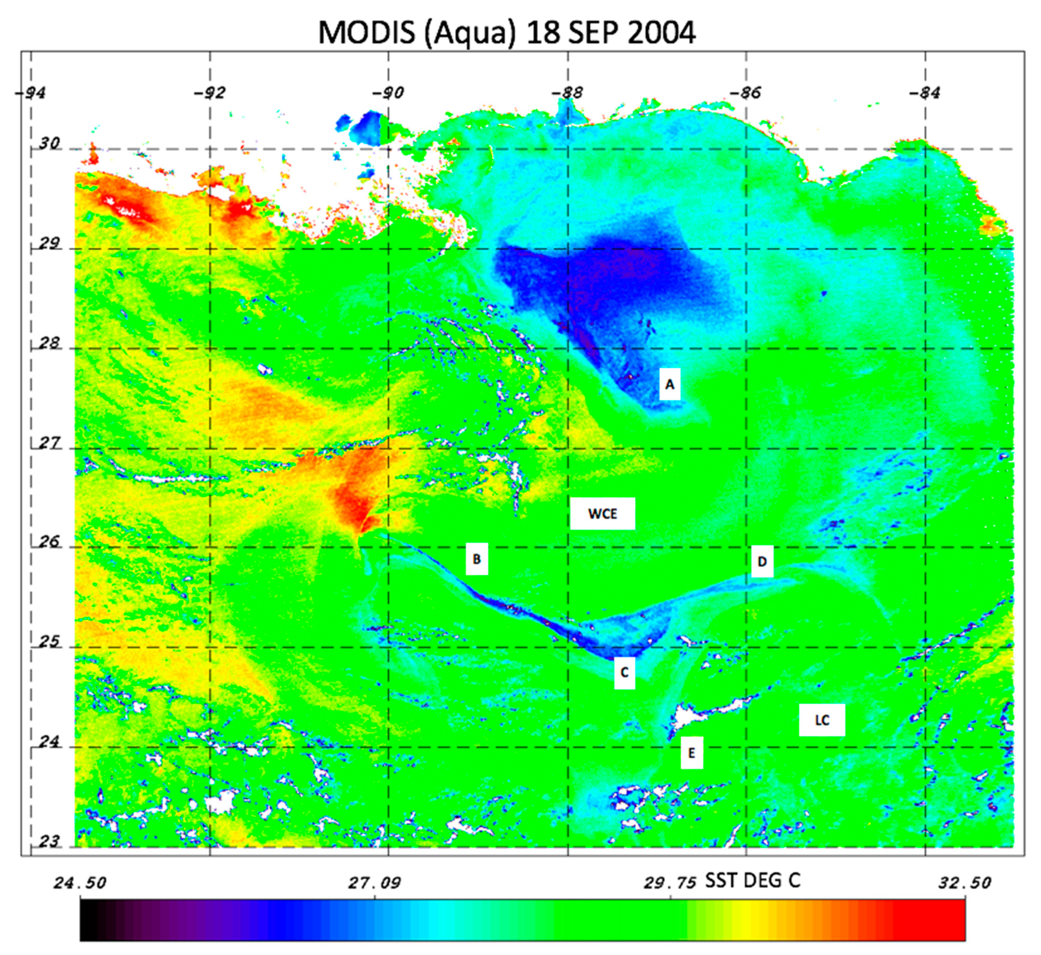
3.2. COAMPS Comparison to Satellite SST and Ocean Color

Verification of the development and subsequent biological activity associated with the aforementioned simulated cold filament is accomplished via MODIS (Aqua) sensor data, collected 18 September 2004. Satellite-estimated surface chlorophyll-a concentration (herein Csat) is elevated throughout the eastern Gulf of Mexico (Figure 10). The following areas are indicated in Figure 10: (A) a broad area to the right of the Ivan track, wherein Csat values are above 0.2 mg m⁻³; (B) an elongated filament of Csat values above 2.0 mg m⁻³, consistent with the location of the COAMPS cold filament; (C) a center of cyclonic circulation between the WCE and LC; (D) apparent filaments of elevated Csat on the periphery of the LC; and (E) elevated Csat on the western side of the LC, as it inters the Gulf and moves past the Campeche Bank. Elevated Csat areas A–D are spatially similar to those resolved by the COAMPS simulations (Figure 8), particularly the cold-Chla filament (B) resolved by the simulation. The COAMPS biological module did not include shelf sediments or river/estuarine effluent of nutrients and bio-optical materials in this experiment; thus, the simulated Chla is strictly due to the open ocean surface ventilation, or shelf upwelling of deeper-water nitrate.

The first solid line contour interval (Figure 10) indicates mesotrophic surface ocean waters. Mesotrophic waters extend from either side of cyclonic circulation area (C) in the form of filaments. A larger area of mesotrophic waters (A) may be due to right-sided mixing/upwelling in the Ivan wake, as well as a pre-existing cyclonic circulation center that is analyzed in more detail elsewhere [1]. This area appears to merge, however, with eutrophic waters extending along the northern Gulf coastlines, and may be due to a combination of estuarine effluent, sediment resuspension, and shelf upwelling interacting with bottom sediments (benthic/pelagic coupling).

Shelf upwelling, shelf sediment and organo-mineral aggregate resuspension, and lateral advection of river/estuarine effluent are all probable contributors to coastal and shelf optical signals in the aftermath of a TC [42]. It is difficult to distinguish these shelf processes in satellite visible-band radiometer data from the signals indicative of strictly open ocean upwelling that are often observed in the wake of cyclones [43]. Deeper waters that upwell onto the shelf will likely mix with sediments from either the bottom or those discharged in river effluent. This is an important optical discriminator because inorganic suspended sediments, especially clay, exhibit strong backscattering characteristics of incident light [44,45], whereas the pelagic suspended particles (primarily the organic matter associated with phytoplankton) exhibit comparatively weaker backscattering [46]. A notable exception to this trend would be open ocean blooms of coccolithophorids [47]. It has also been previously argued that, in some instances, tropical cyclones or significant flooding/rainfall events may result in the advection of low-salinity coastal waters to several hundred kilometers away from the coast [2,48].

The MODIS sea surface temperature (SST) product provides additional clarity on the underlying biophysical mechanisms resulting in the observed Csat distribution (Figure 10), particularly where it appears to match the COAMPS biophysical simulation. Areas A–D are all consistent with an SST depression to less than 27 °C (Figure 11), indicative of surface ventilation of deeper waters. There is only patchy SST depression in area (E), as it is likely a result of LC interaction with the Campeche Bank. In the other areas, however, the SST depression is conspicuous, and particularly so along the elongated westward filament (Area B; Figure 11). The meridional thickness of the SST filament depression (< 27 °C) at 88.5° W (cross-filament direction) is ~ 7 km. The MODIS SST and Csat data show the westward filament was developed by 18 September and extended between ~ 25°–26° N, whereas the COAMPS simulation delayed westward filament evolution until 19 September and it occurs at approximately 0.5 degrees latitude farther south. Despite these spatio-temporal imperfections, the COAMPS results suggest that similar biophysical dynamics are responsible for the “real-world” satellite observations, i.e., a submesoscale cold filament between the anticyclonic centers of circulation that results in mesotrophic surface water conditions.

An alternative method to detect potential optical differences in surface water masses (and discover clues to their biogeochemical histories) is to render the MODIS multispectral data as a true color image, following the colorimetry method described in Section 2.2. The resulting true color image indicates dark green (low brightness) along the southern and northern peripheries of the WCE (Figure 12, areas A–C). This is precisely where the SST field shows depressed temperatures and approximately where the COAMPS simulation (Figure 8), devoid of simulated shelf sediments and river effluent, indicated open ocean upwelling that would result in the elevated phytoplankton and organic matter concentration. On the southern flank of the WCE, the brighter color patterns farther south towards the Yucatan Peninsula, suggest either shelf water advection or shelf-break upwelling from the adjacent Campeche Bank. To the north (Area A), there is a distinct color gradient that potentially demarcates the boundary between the shelf-influenced waters (bright) and the open ocean upwelling signal (dark).

4. Discussion

Cold wake upwelling/entrainment of deeper, cooler waters on the right-hand side of the TC path has been well documented and simulated [31,49,50,51]. Intense momentum flux from the atmosphere to the ocean results in turbulent overturning of the upper water column and entrainment of deeper waters into the surface mixed layer. Resonance between inertial current oscillations and wind stress creates a right-sided cold bias along the storm track [6,52]. These processes will, in turn, stimulate phytoplankton productivity as nutrients are upwelled into the euphotic zone and vertical stability is re-established [8].

In addition to rightward (northern hemisphere) asymmetric cooling, the TC will also modulate the existing mesoscale eddy field and elicit a biophysical response [10,53]. It has been demonstrated that in the Gulf of Mexico, the cold core (cyclonic) circulation centers’ upper ocean current velocity response to the TC near-inertial wave wake is nearly twice as large as in anticyclones [54,55], thus the spatial distribution of the TC wake cooling may be strongly influenced by the pre-existing distribution of the WCE and CCE circulation centers. Satellite observation and model tracer studies of the aftermath of GOM Hurricane Katrina (2005) show enhanced cooling and primary productivity within a CCE that was located to the left of the storm track [56].

At the time of Hurricane Ivan’s transit through the Gulf, a large WCE had just separated from the LC and a smaller CCE circulation center emerged between the two features, as is common during the WCE–LC separation process [57,58]. It is likely that the near-inertial wave wake intensified the CCE circulation and amplified the TC cooling impact there, and thus a substantially amplified density gradient was imposed across the boundary between mesoscale circulation features. The COAMPS biophysical simulation then resolved a westward propagating cold/chlorophyll filament on the edge of the WCE circulation that conforms to submesoscale dynamics. A remarkably similar feature is seen in both satellite SST and chlorophyll data.

Thus, our simulations suggest that in addition to right sided asymmetry and CCE intensification/cooling, a separable and submesoscale biological–physical process may evolve in the aftermath of a TC passage. This also suggests that horizontally propagating “filaments” of discolored water (or high satellite-estimated chlorophyll) that appear in satellite ocean color images of the Gulf of Mexico may not always be the result of horizontal advection of shelf waters [2,59], but may instead be the result of frontogenetic instability along the periphery of mesoscale circulation features. These submesoscale filaments are brought about by a fundamentally different biophysical process, through which nitrogen-rich, colder waters can be brought to the ocean surface to promote enhanced primary productivity via ageostrophic vertical circulation. The spatial confluence of these features with the mesoscale flow field, and their apparent growth in a sequence of satellite images, may give the misleading impression that sea surface properties (chlorophyll/temperature) are largely being horizontally advected around the anticyclonic circulation centers.

What does indeed appear to propagate around the anticyclonic circulation centers in the COAMPS simulation are very elevated rates of horizontal strain (Figure 4a), as a persistent result of the TC inertial energy imparted to the surface ocean. The “classic frontogenetic process” [40] occurs under the circumstances of such an elevated surface strain and often between cores of mesoscale circulation [60,61]. The satellite-detected cold filament emphasized herein appears to evolve much more rapidly and narrowly than in the COAMPS simulations. We speculate that the simulated cold filament development is likely impeded, and then subsequently arrested, due to the limitations imposed by the hydrostatic ocean model’s horizontal grid resolution (~ 2 km) and imperfect representations of turbulence [62].

Huang and Oey [63] also provided biophysical modeling evidence for submesoscale processes in the wake of TC passage. Their results suggest that submesoscale effects primarily associated with resonant Reynolds stresses tend to amplify the observed right-sided biophysical response along the TC path. Our results show that the amplification of lateral strain and relative vorticity along the periphery of the existing mesoscale circulation features may propagate filaments, irrespective of the prototypical rightward asymmetry of the ocean’s TC response. The inertial energy imparted by TC passage may render this general process (i.e., strain field frontogenesis along the periphery of mesoscale circulation features) conspicuous enough for satellite observation and modeling studies. However, more frequent meteorological events, such as atmospheric fontal passage, may also stimulate similar oceanic processes. Our results strongly support the hypothesis [32] that these submesoscale biophysical processes may have cumulatively large impacts on the overall productivity of the oceans.

References

1. Walker, N.D.; Leben, R.R.; Balasubramanian, S. Hurricane-forced upwelling and chlorophyll a enhancement within cold-core cyclones in the Gulf of Mexico. Geophys. Res. Lett. 2005, 32. [Google Scholar] [CrossRef]
2. Kil, B.; Wiggert, J.D.; Howden, S.D. Evidence That an Optical Tail in the Gulf of Mexico After Tropical Cyclone Isaac was the Result of Offshore Advection of Coastal Water. Mar. Technol. Soc. J. 2014, 48, 27–35. [Google Scholar] [CrossRef]
3. Walker, N.D.; Huh, O.K.; Rouse, L.J., Jr.; Murray, S.P. Evolution and structure of a coastal squirt off the Mississippi River delta: Northern Gulf of Mexico. J. Geophys. Res. 1996, 101, 20643–20655. [Google Scholar] [CrossRef]
4. Son, Y.B.; Gardner, W.B.; Richardson, M.J.; Ishizaka, J.; Ryu, J.-H.; Kim, S.-H.; Lee, S.H. Tracing offshore low-salinity plumes in the Northeastern Gulf of Mexico during the summer season by use of multi-spectral remote sensing data. J. Oceanogr. 2012, 68, 743–760. [Google Scholar] [CrossRef]
5. Price, J.F. Upper ocean response to a hurricane. J. Phys. Oceanogr. 1981, 11, 153–175. [Google Scholar] [CrossRef]
6. Shay, L.K.; Mariano, A.J.; Jacob, S.D.; Ryan, E.H. Mean and Near-Inertial Ocean Current Response to Hurricane Gilbert. J. Phys. Oceanogr. 1998, 28, 858–889. [Google Scholar] [CrossRef]
7. Prasad, T.G.; Hogan, P.J. Upper-ocean response to Hurricane Ivan in a 1/25° nested Gulf of Mexico HYCOM. J. Geophys. Res. Ocean. 2007, 112. [Google Scholar] [CrossRef]
8. Babin, S.M.; Carton, J.A.; Dickey, T.D.; Wiggert, J.D. Satellite evidence of hurricane-induced phytoplankton blooms in an oceanic desert. J. Geophys. Res. Ocean. 2004, 109. [Google Scholar] [CrossRef]
9. Hu, C.; Muller-Karger, F.E. Response of sea surface properties to Hurricane Dennis in the eastern Gulf of Mexico. Geophys. Res. Lett. 2007, 34. [Google Scholar] [CrossRef]
10. Chen, Y.; Tang, D. Eddy-feature phytoplankton bloom induced by a tropical cyclone in the South China Sea. Int. J. Remote Sens. 2012, 33, 7444–7457. [Google Scholar] [CrossRef]
11. Merritt-Takeuchi, A.M.; Chiao, S. Case Studies of Tropical Cyclones and Phytoplankton Blooms over Atlantic and Pacific Regions. Earth Interact. 2013, 17, 1–19. [Google Scholar] [CrossRef] [Green Version]
12. Doyle, J.D.; Hodue, R.M.; Chen, S.; Jin, Y.; Moskatis, J.R.; Wang, S.; Hendricks, E.A.; Jin, H.; Smith, T.A. Tropical Cylone Prediction Using COAMPS-TC. Oceanography 2014, 27, 104–115. [Google Scholar] [CrossRef]
13. Smith, T.A.; Chen, S.; Campbell, T.; Martin, P.; Rogers, W.E.; Gaberšek, S.; Wang, D.; Carroll, S.; Allard, R. Ocean–wave coupled modeling in COAMPS-TC: A study of Hurricane Ivan (2004). Ocean Model. 2013, 69, 181–194. [Google Scholar] [CrossRef]
14. McWilliams, J.C. Submesoscale currents in the ocean. Proc. R. Soc. A: Math. Phys. Eng. Sci. 2016, 472, 20160117. [Google Scholar] [CrossRef]
15. Petrenko, A.A.; Doglioli, A.M.; Nencioli, F.; Kersalé, M.; Hu, Z.; d’Ovidio, F. A review of the LATEX project: Mesoscale to submesoscale processes in a coastal environment. Ocean Dyn. 2017, 67, 513–533. [Google Scholar] [CrossRef]
16. Ramachandran, S.; Tandon, A.; Mahadevan, A. Enhancement in vertical fluxes at a front by mesoscale-submesoscale coupling. J. Geophys. Res. Ocean. 2014, 119, 8495–8511. [Google Scholar] [CrossRef] [Green Version]
17. Oguz, T.; Macias, D.; Tintore, J. Ageostrophic Frontal Processes Controlling Phytoplankton Production in the Catalano-Balearic Sea (Western Mediterranean). PLoS ONE 2015, 10, e0129045. [Google Scholar] [CrossRef]
18. Thomas, E.R.; João, T.; Melinda, P.; Timothy, F.H.; Randal, P. Navy Operational Global Atmospheric Prediction System (NOGAPS): Forcing for Ocean Models. Oceanography 2002, 15, 99–108. [Google Scholar] [Green Version]
19. Daley, R.; Barker, E. NAVDAS: Formulation and Diagnostics. Mon. Weather Rev. 2001, 129, 869–883. [Google Scholar] [CrossRef]
20. Chen, S.; Campbell, T.J.; Jin, H.; Gaberšek, S.; Hodur, R.M.; Martin, P. Effect of Two-Way Air–Sea Coupling in High and Low Wind Speed Regimes. Mon. Weather Rev. 2010, 138, 3579–3602. [Google Scholar] [CrossRef]
21. Martin, P.J. Description of the Nacy Coastal Ocean Model 1.0; Naval Research Lab Stennis Space Center Ms: Stennis Space Center, MS, USA, 2000; p. 45. [Google Scholar]
22. Barron, C.N.; Kara, A.B.; Hurlburt, H.E.; Rowley, C.; Smedstad, L.F. Sea surface height predictions from the Global Navy Coastal Ocean Model (NCOM) during 1998–2001. J. Atmos. Ocean. Technol. 2004, 21, 1876–1894. [Google Scholar] [CrossRef]
23. Fox, D.N.; Teague, W.J.; Barron, C.N.; Carnes, M.R.; Lee, C.M. The Modular Ocean Data Assimilation System (MODAS). J. Atmos. Ocean. Technol. 2002, 19, 240–252. [Google Scholar] [CrossRef]
24. Jolliff, J.K.; Kindle, J.C.; Penta, B.; Helber, R.; Lee, Z.; Shulman, I.; Arnone, R.A.; Rowley, C. On the relationship between satellite-estimated bio-optical and thermal properties in the Gulf of Mexico. J. Geophys. Res. Biogeosci. 2008, 113, G010204. [Google Scholar] [CrossRef]
25. Jolliff, J.K.; Smith, T.A. Biological modulation of upper ocean physics: Simulating the biothermal feedback effect in Monterey Bay, California. J. Geophys. Res. Biogeosci. 2014, 119, 703–721. [Google Scholar] [CrossRef]
26. Ladner, S.; Crout, R.; Lawson, A.; Martinolich, P.M.; Bowers, J.; Arnone, R.A. Validation Test Report for the Automated Optical Processing System (AOPS) Version 16; U.S. Naval Research Laboratory: Washington, DC, USA, 2016. [Google Scholar]
27. NASA Ocean Biology Processing Group, Group, Chlorophyll a (chlor_a) Product Description. Available online: https://oceancolor.gsfc.nasa.gov/atbd/chlor_a/ (accessed on 17 July 2019).
28. Hu, C.; Lee, Z.; Franz, B. Chlorophyll aalgorithms for oligotrophic oceans: A novel approach based on three-band reflectance difference. J. Geophys. Res. Ocean. 2012, 117. [Google Scholar] [CrossRef]
29. Wernand, M.R.; Hommersom, A.; Van der Woerd, H.J. MERIS-based ocean colour classification with the discrete Forel-Ule scale. Ocean Sci. 2013, 9, 477–487. [Google Scholar] [CrossRef]
30. Jolliff, K.J.; Lewis, D.M.; Ladner, S.; Crout, L.R. Observing the Ocean Submesoscale with Enhanced-Color GOES-ABI Visible Band Data. Sensors 2019, 19. [Google Scholar] [CrossRef]
31. Price, J.F.; Sanford, T.B.; Forristall, G.Z. Forced stage response to a moving hurricane. J. Phys. Oceanogr. 1994, 24, 233–260. [Google Scholar] [CrossRef]
32. Mahadevan, A. The Impact of Submesoscale Physics on Primary Productivity of Plankton. Annu. Rev. Mar. Sci. 2016, 8, 161–184. [Google Scholar] [CrossRef] [Green Version]
33. Okubo, A. Horizontal dispersion of floatable particles in the vicinity of velocity singularities such as convergences. Deep Sea Res. Oceanogr. Abstr. 1970, 17, 445–454. [Google Scholar] [CrossRef]
34. Weiss, J. The dynamics of enstrophy transfer in two-dimensional hydrodynamics. Phys. D Nonlinear Phenom. 1991, 48, 273–294. [Google Scholar] [CrossRef]
35. Mahadevan, A.; Tandon, A. An analysis of mechanisms for submesoscale vertical motion at ocean fronts. Ocean Model. 2006, 14, 241–256. [Google Scholar] [CrossRef]
36. Mahadevan, A. Submesoscale Processes. In Encyclopedia of Ocean Sciences, 3rd ed.; Elsevier: Amsterdam, The Netherlands, 2019; Volume 1, pp. 35–41. [Google Scholar]
37. Gula, J.; Molemaker, M.J.; McWilliams, J.C. Submesoscale Dynamics of a Gulf Stream Frontal Eddy in the South Atlantic Bight. J. Phys. Oceanogr. 2015, 46, 305–325. [Google Scholar] [CrossRef]
38. Ochoa, J.; Sheinbaum, J.; Badan, A.; Candela, J.; Wilson, D. Geostrophy via potential vorticity inversion in the Yucatan Channel. J. Mar. Res. 2001, 59, 725–747. [Google Scholar] [CrossRef]
39. Thomas, L.N.; Tandon, A.; Mahadevan, A. Submesoscale processes and dynamics. In Ocean Modeling in an Eddying Regime; Hecht, M.W., Hasumi, H., Eds.; AGU, Geophysical Monograph Series: Washington, DC, USA, 2007. [Google Scholar] [CrossRef]
40. Sullivan, P.P.; McWilliams, J.C. Frontogenesis and frontal arrest of a dense filament in the oceanic surface boundary layer. J. Fluid Mech. 2018, 837, 341–380. [Google Scholar] [CrossRef]
41. Gula, J.; Molemaker, M.J.; McWilliams, J.C. Submesoscale Cold Filaments in the Gulf Stream. J. Phys. Oceanogr. 2014, 44, 2617–2643. [Google Scholar] [CrossRef]
42. Halper, F.B.; Schroeder, W.W. The response of shelf waters to the passage of tropical cyclones—Observations from the Gulf of Mexico. Cont. Shelf Res. 1990, 10, 777–793. [Google Scholar] [CrossRef]
43. Hoge, F.E.; Lyon, P.E. Satellite observation of Chromophoric Dissolved Organic Matter (CDOM) variability in the wake of hurricanes and typhoons. Geophys. Res. Lett. 2002, 29, 1908. [Google Scholar] [CrossRef]
44. Chen, M.S.; Wartel, S.; Eck, B.V.; Maldegem, D.V. Suspended matter in the Scheldt estuary. Hydrobiologia 2005, 540, 79–104. [Google Scholar] [CrossRef]
45. Knaeps, E.; Ruddick, K.G.; Doxaran, D.; Dogliotti, A.I.; Nechad, B.; Raymaekers, D.; Sterckx, S. A SWIR based algorithm to retrieve total suspended matter in extremely turbid waters. Remote Sens. Environ. 2015, 168, 66–79. [Google Scholar] [CrossRef] [Green Version]
46. Stramski, D.; Boss, E.; Bogucki, D.; Voss, K.J. The role of seawater constituents in light backscattering in the ocean. Prog. Oceanogr. 2004, 61, 27–56. [Google Scholar] [CrossRef]
47. Balch, W.M.; Kilpatrick, K.A.; Trees, C.C. The 1991 coccolithophore bloom in the central North Atlantic. 1. Optical properties and factors affecting their distribution. Limnol. Oceanogr. 1996, 41, 1669–1683. [Google Scholar] [CrossRef]
48. Gierach, M.M.; Vazquez-Cuervo, J.; Lee, T.; Tsontos, V.M. Aquarius and SMOS detect effects of an extreme Mississippi River flooding event in the Gulf of Mexico. Geophys. Res. Lett. 2013, 40, 5188–5193. [Google Scholar] [CrossRef]
49. Shang, S.; Li, L.; Sun, F.; Wu, J.; Hu, C.; Chen, D.; Ning, X.; Qiu, Y.; Zhang, C.; Shang, S. Changes of temperature and bio-optical properties in the South China Sea in response to Typhoon Lingling, 2001. Geophys. Res. Lett. 2008, 35. [Google Scholar] [CrossRef] [Green Version]
50. Chiang, T.-L.; Wu, C.-R.; Oey, L.-Y. Typhoon Kai-Tak: An Ocean’s Perfect Storm. J. Phys. Oceanogr. 2010, 41, 221–233. [Google Scholar] [CrossRef]
51. Li, H.; Sriver, R.L. Impact of Tropical Cyclones on the Global Ocean: Results from Multidecadal Global Ocean Simulations Isolating Tropical Cyclone Forcing. J. Clim. 2018, 31, 8761–8784. [Google Scholar] [CrossRef]
52. Shay, L.K.; Elsberry, R.L. Near-Inertial Ocean Current Response to Hurricane Frederic. J. Phys. Oceanogr. 1987, 17, 1249–1269. [Google Scholar] [CrossRef]
53. Zheng, Z.-W.; Ho, C.-R.; Zheng, Q.; Lo, Y.-T.; Kuo, N.-J.; Gopalakrishnan, G. Effects of preexisting cyclonic eddies on upper ocean responses to Category 5 typhoons in the western North Pacific. J. Geophys. Res. Ocean. 2010, 115. [Google Scholar] [CrossRef]
54. Jaimes, B.; Shay, L.K. Mixed Layer Cooling in Mesoscale Oceanic Eddies during Hurricanes Katrina and Rita. Mon. Weather Rev. 2009, 137, 4188–4207. [Google Scholar] [CrossRef] [Green Version]
55. Jaimes, B.; Shay, L.K. Near-Inertial Wave Wake of Hurricanes Katrina and Rita over Mesoscale Oceanic Eddies. J. Phys. Oceanogr. 2010, 40, 1320–1337. [Google Scholar] [CrossRef]
56. Liu, X.; Wang, M.; Shi, W. A study of a Hurricane Katrina–induced phytoplankton bloom using satellite observations and model simulations. J. Geophys. Res. Ocean. 2009, 114. [Google Scholar] [CrossRef]
57. Biggs, D.C.; Fargion, G.S.; Hamilton, P.; Leben, R. Cleavage of a Gulf of Mexico Loop Current eddy by a deep water cyclone. J. Geophys. Res. 1996, 101, 20629–20641. [Google Scholar] [CrossRef]
58. Sturges, W.; Leben, R. Frequency of Ring seperations from the Loop Current in the Gulf of Mexico. J. Phys. Oceanogr. 2000, 30, 1814–1819. [Google Scholar] [CrossRef]
59. Lohrenz, S.E.; Cai, W.-J.; Chen, X.; Tuel, M. Satellite Assessment of Bio-Optical Properties of Northern Gulf of Mexico Coastal Waters Following Hurricanes Katrina and Rita. Sensors 2008, 8, 4135–4150. [Google Scholar] [CrossRef] [PubMed] [Green Version]
60. Hoskins, B.J. The Mathematical Theory of Frontogenesis. Annu. Rev. Fluid Mech. 1982, 14, 131–151. [Google Scholar] [CrossRef]
61. McWilliams, J.C.; Colas, F.; Molemaker, M.J. Cold filamentary intensification and oceanic surface convergence lines. Geophys. Res. Lett. 2009, 36. [Google Scholar] [CrossRef]
62. McWilliams, J.C.; Gula, J.; Molemaker, M.J.; Renault, L.; Shchepetkin, A.F. Filament Frontogenesis by Boundary Layer Turbulence. J. Phys. Oceanogr. 2015, 45, 1988–2005. [Google Scholar] [CrossRef]
63. Huang, S.M.; Oey, L.-Y. Right-side cooling and phytoplankton bloom in the wake of a tropical cyclone. J. Geophys. Res. Ocean. 2015, 120, 5735–5748. [Google Scholar] [CrossRef]
Figure 1. (A) GOES-12 visible satellite image of Hurricane Ivan from 16 September 2004, nearing landfall along the northern GOM coast. (B) COAMPS-TC wind speed (shaded) and direction (black vectors) for 0000 UTC September 15 2014 are plotted. Actual track is shown by the purple line and each waypoint represents Ivan’s center position every 12 h, at 0000 and 1200 UTC each day.
Jmse 07 00378 g001
Figure 2. Sea surface height on (a) 13 September 2004 and (b) 17 September 2004. Positive SSH (purple contours) and negative SSH (red contours) are shown (0.05 m intervals). The warm core eddy (WCE), Loop Current (LC), and Cold core eddy (CCE) are labeled. Hurricane Ivan’s track is indicated by the dark purple line, with waypoints at each 0000 and 1200 UTC location. The primary track of interest is from 14 September 2004 until 16 September 2004, when Ivan entered the Gulf of Mexico and made landfall near Pensacola, FL.
Jmse 07 00378 g002
Figure 3. COAMPS-TC sea surface temperature (°C) between 85°-92° W and 22.5°–26.5° N. (a) 0000 UTC 13 September 2004. (b) 0000 UTC 17 September 2004. (c) 0000 UTC 19 September 2004. (d) 0000 UTC 20 September 2004. The Hurricane Ivan track is indicated by the dark purple line, with waypoints at each 0000 and 1200 UTC location.
Jmse 07 00378 g003
Figure 4. (a) Surface strain (s−1) at the surface for 0000 UTC 20 September 2004 and (b) Surface vorticity (s−1) at 0000 UTC 20 September 2004. Vectors represent surface currents’ strength and direction. Hurricane Ivan track is indicated by the dark purple line, with waypoints at each 0000 and 1200 UTC location. The blue shaded area represents the primary area of interest including, and surrounding, the filament.
Jmse 07 00378 g004
Figure 5. Okubo–Weiss parameter (shaded) for (a) 0000 UTC 13 September 2004 and (b) 0000 UTC 20 September 2004. Vectors represent surface currents’ strength and direction. Hurricane Ivan track is indicated by the dark purple line, with waypoints at each 0000 and 1200 UTC location. The blue shaded area represents the primary area of interest surrounding the filament.
Jmse 07 00378 g005
Figure 6. Simulated filament cross-section view (~89.6° W), outer filament edge 20 September 2004: (a) strain rate (s−1); (b) vertical velocities (m s−1); (c) relative vorticity (s−1); (d) temperature (°C); (e) chlorophyll (mg m−3) logarithmic scale; (f) nitrate (mmol N m−3). Chlorophyll concentration contours are overlain on each panel, depth axis is down to 200 m.
Jmse 07 00378 g006
Figure 7. Simulated filament cross-section view (~88.2° W), outer filament edge 20 September 2004: (a) strain rate (s−1); (b) vertical velocities (m s−1); (c) relative vorticity (s−1); (d) temperature (°C); (e) chlorophyll (mg m−3); (f) nitrate (mmol N m−3). Chlorophyll concentration contours are overlain on each panel, depth axis is down to 100 m.
Jmse 07 00378 g007
Figure 8. Simulated surface chlorophyll on 0000 UTC September 19–21. Simulated SSH is overlain in solid contours. Cross-section plots (Figure 6, Figure 7 and Figure 9) correspond to lines shown across the filament on the southern edge of the WCE.
Jmse 07 00378 g008
Figure 9. Simulated filament cross-section view (~89.6° W), outer filament edge 21 September 2004: (a) strain rate (s−1); (b) vertical velocities (m s−1); (c) relative vorticity (s−1); (d) temperature (°C); (e) chlorophyll (mg m−3); (f) nitrate (mmol N m−3). Chlorophyll concentration contours are overlain on each panel, depth axis is down to 100 m.
Jmse 07 00378 g009
Figure 10. MODIS (Aqua) Csat product on 18 SEP 04. Lettered areas are referenced in the text. WCE indicates warm core eddy–anticyclonic circulation center, LC indicates Loop Current. Labeled areas are as follows: (A) large domain of right-sided TC SST reduction; (B) westward propagating cold filament; (C) CCE; (D) eastward cold filaments along LC edge; (E) area of likely LC-shelf (Campeche Bank) interaction.
Jmse 07 00378 g010
Figure 11. MODIS SST product for 18 September 2004. Labeled areas are as in Figure 10.
Jmse 07 00378 g011
Figure 12. MODIS (Aqua) True Color (colorimetry method) corresponding to Figure 10 and Figure 11. Labeled areas are as in Figure 10 and Figure 11.
Jmse 07 00378 g012